Deep Neural Networks for ECG-Based Pulse Detection during Out-of-Hospital Cardiac Arrest

Abstract

The automatic detection of pulse during out-of-hospital cardiac arrest (OHCA) is necessary for the early recognition of the arrest and the detection of return of spontaneous circulation (end of the arrest). The only signal available in every single defibrillator and valid for the detection of pulse is the electrocardiogram (ECG). In this study we propose two deep neural network (DNN) architectures to detect pulse using short ECG segments (5 s), i.e., to classify the rhythm into pulseless electrical activity (PEA) or pulse-generating rhythm (PR). A total of 3914 5-s ECG segments, 2372 PR and 1542 PEA, were extracted from 279 OHCA episodes. Data were partitioned patient-wise into training (80%) and test (20%) sets. The first DNN architecture was a fully convolutional neural network, and the second architecture added a recurrent layer to learn temporal dependencies. Both DNN architectures were tuned using Bayesian optimization, and the results for the test set were compared to state-of-the art PR/PEA discrimination algorithms based on machine learning and hand crafted features. The PR/PEA classifiers were evaluated in terms of sensitivity (Se) for PR, specificity (Sp) for PEA, and the balanced accuracy (BAC), the average of Se and Sp. The Se/Sp/BAC of the DNN architectures were 94.1%/92.9%/93.5% for the first one, and 95.5%/91.6%/93.5% for the second one. Both architectures improved the performance of state of the art methods by more than 1.5 points in BAC.

1. Introduction

Out-of-hospital cardiac arrest (OHCA) remains a major public health problem, with 350,000–700,000 individuals per year affected in Europe and survival rates below 10% [1,2]. Early recognition of OHCA is key for survival [3] as it allows a rapid activation of the emergency system and facilitates bystander cardiopulmonary resuscitation (CPR). Bystanders should apply an automated external defibrillator (AED), designed to be used with minimal training and to guide the rescuer until the arrival of medical personnel [4]. The main goal of OHCA treatment is to achieve return of spontaneous circulation (ROSC), so that post-resuscitation care can be initiated and the patient can be transported to hospital. Early recognition and post-resuscitation care are two key factors for the survival of the patient, and both these factors require the accurate detection of presence/absence of pulse.

Nowadays, healthcare professionals check for pulse by manual palpation of the carotid artery or by looking for signs of life. However, carotid pulse palpation has been proven inaccurate (specificity 55%) and time consuming (median delays of 24 s) for both bystanders and healthcare personnel [5,6,7,8,9]. Consequently, current resuscitation guidelines recommend the assessment of carotid pulse together with looking for signs of life only for experienced people [10]. Checking for signs of life alone has not been proven to be more accurate. In fact, healthcare personnel show difficulties when discriminating between normal (pulse present) and agonal (absence of pulse) breathing [11,12]. More modern approaches use ultrasound to visually assess the mechanical activity of the heart and detect pulse-generating rhythms accurately [13]. Unfortunately, the required equipment is not available during bystander CPR and very rarely for medical personnel in the out-of-hospital setting. Besides, some studies suggest that the use of ultrasound lengthens the duration of chest compression pauses [14,15], decreasing the probability of survival of the patient. Automatic accurate pulse detectors are still needed to assist the rescuer in monitoring the hemodynamic state of the patient [16].

Cardiac arrest rhythms are grouped into the following 4 categories [10]: ventricular fibrillation (VF), ventricular tachycardia (VT), asystole (AS), and pulseless electrical activity (PEA). When ROSC is achieved the patient shows a pulse-generating rhythm (PR). VF and VT need a defibrillation, and a vast number of algorithms have been proposed to detect them [17,18,19,20]. Among non-shockable rhythms, AS is defined as the absence of electrical and mechanical activity of the heart. PEA shows an organized electrical activity of the heart but no clinically palpable pulse, i.e., the mechanical activity is not efficient enough to maintain the consciousness of the patient [21]. AS rhythms can be discriminated using features that are sensitive to amplitude [22], so the most challenging scenario for pulse detection is the discrimination between PR and PEA rhythms. A precise PR/PEA discrimination would allow an earlier recognition of the arrest, and also the identification of ROSC when treating the OHCA patient.

In the last two decades many efforts have been dedicated to automated methods for PR/PEA discrimination based on several non-invasive biomedical signals monitored by defibrillators. The thoracic impedance (TI) shows small fluctuations (≈40 m$\mathsf{\Omega }$) with each effective heartbeat [23,24,25], so it has been proposed for pulse detection alone [26,27] or in combination with the ECG [28,29]. However, many commercial defibrillators do not have enough amplitude resolution to detect TI fluctuations produced by effective heartbeats, and the methods have not been proven to be reliable during ventilations because of the TI fluctuations produced by air insufflation [29]. Other signals such as the photoplethysmogram [30,31], capnogram [32], or acceleration [33] have been also included in algorithms for PR/PEA discrimination, but these signals are not commonly available in all monitor/defibrillators. Instead, the ECG acquired using the defibrillation pads is available in all defibrillators, and algorithms based exclusively on the ECG could be of universal use, and easy to integrate in any device.

The main objective of this study was to develop a pulse detection algorithm based exclusively on the ECG acquired by defibrillation pads. Previously a machine learning technique was proposed using a random forest (RF) classifier based on hand-crafted features [34]. Alternatively, deep neural networks (DNN) have shown superior performance in classification problems with large datasets in many fields [35,36,37,38]. DNN solutions have no need of feature engineering as the signals are directly fed to the network which does the exploratory data analysis. Convolutional neural networks (CNN) have been successfully used for heartbeat arrhythmia classification [39,40,41] or the detection of myocardial affections [42,43], and recurrent neural networks (RNN) have been proven accurate for diagnostic applications when time dependencies in the signal are important [44,45]. This work proposes and compares various DNN solutions for PR/PEA classification. The manuscript is organized as follows: Section 2 describes the data used in this study; in Section 3 the proposed DNN solutions are described; classical machine learning based approaches are described in Section 4 and used for comparison; Section 5 describes the optimization process of the models and the evaluation methods applied; and in Section 6 and Section 7 the results are presented and discussed.

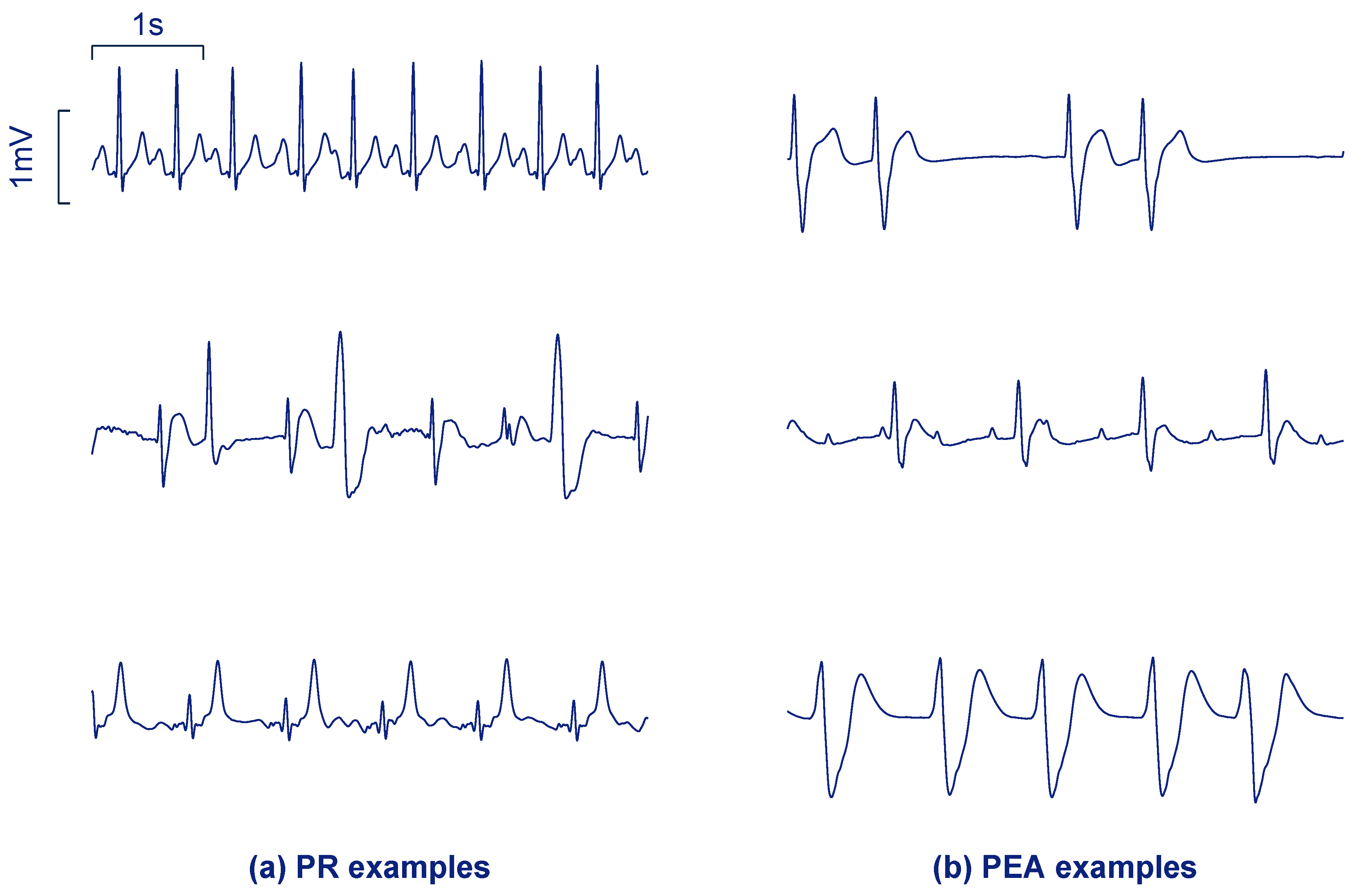
2. Data Collection

The data of the study were a subset of a large OHCA episode collection gathered by the DFW centre for resuscitation research (UTSW, Dallas). Every episode was recorded using the Philips HeartStart MRx device, which acquires the ECG signal through defibrillation pads with a sampling frequency of 250 Hz and a resolution of 1.03 $\mathsf{\mu }$V per least significant bit.

There were a total of 1561 episodes of which 1015 contained concurrent ECG and TI signals. The TI signal was necessary to identify ECG intervals free of artefacts due to chest compressions provided to the patient during CPR. Episodes were separated in ROSC and no-ROSC groups based on the instant of ROSC annotated by the clinicians on scene. PEA rhythms were extracted from no-ROSC patients. PR rhythms were extracted after the instant of ROSC for patients who showed sustained ROSC.

ECG segments of 5 s were automatically extracted during intervals without chest compressions. Chest compressions were automatically detected in the TI using the algorithm proposed in [46], or in the compression depth signal of the monitor [47]. Then, organized rhythms (PR or PEA) were automatically identified using an offline version of a commercial shock advise algorithm [17]. Three biomedical engineers reviewed the segments to check they contained visible QRS complexes with a minimum rate of 12 bpm. Every segment was annotated as PEA or PR based on the clinical annotations. Consecutive ECG segments were extracted using a minimum separation between segments of 1 s for PEA and 30 s for PR. PEA is more variable than PR, and occurs during the arrest. During PEA, CPR is given to the patient and intervals without compressions are not frequent. After ROSC is identified (PR segments) chest compressions are interrupted, and long intervals of artefact-free ECG are available. A longer separation between PR segments was considered to increase the variability.

A total of 3914 segments (2372 PR and 1542 PEA) from 279 patients (134 with ROSC and 145 without ROSC) comprised the dataset. Patient-wise training and test sets were created ($\approx 80\%/20\%$ of the patients). The training set contained 3038 segments (1871 PR) from 223 patients (105 with ROSC). The test set contained 876 segments (501 PR) from 56 patients (29 with ROSC).

Figure 1 shows examples of three PR segments (panel a) and three PEA segments (panel b). PR usually shows higher rates, narrower QRS complexes, less heart rate variability and higher frequency content (steeper QRS complexes) than PEA. However, PR in cardiac arrest often shows irregular beats as in the last two examples of Figure 1a. PEA rhythms may show more aberrant QRS complexes, absence of P waves, or more ectopic heartbeats compared to PR.

3. Proposed DNN Architectures

Two DNN architectures were implemented for the binary classification of ECG into PR/PEA. The 5 s ECG segments were first bandpass filtered using the typical AED bandwidth (0.5–30 Hz). The filtered ECG was downsampled to 100 Hz to obtain $s\left[n\right]$, a signal of $N=500$ samples, that was fed to the DNN networks. The output of the networks was $p_{PR}\in (0,1)$, the likelihood that a 5 s segment corresponds to a PR segment. The first solution we propose is a fully convolutional neural network, and the second solution integrates recurrent layers.

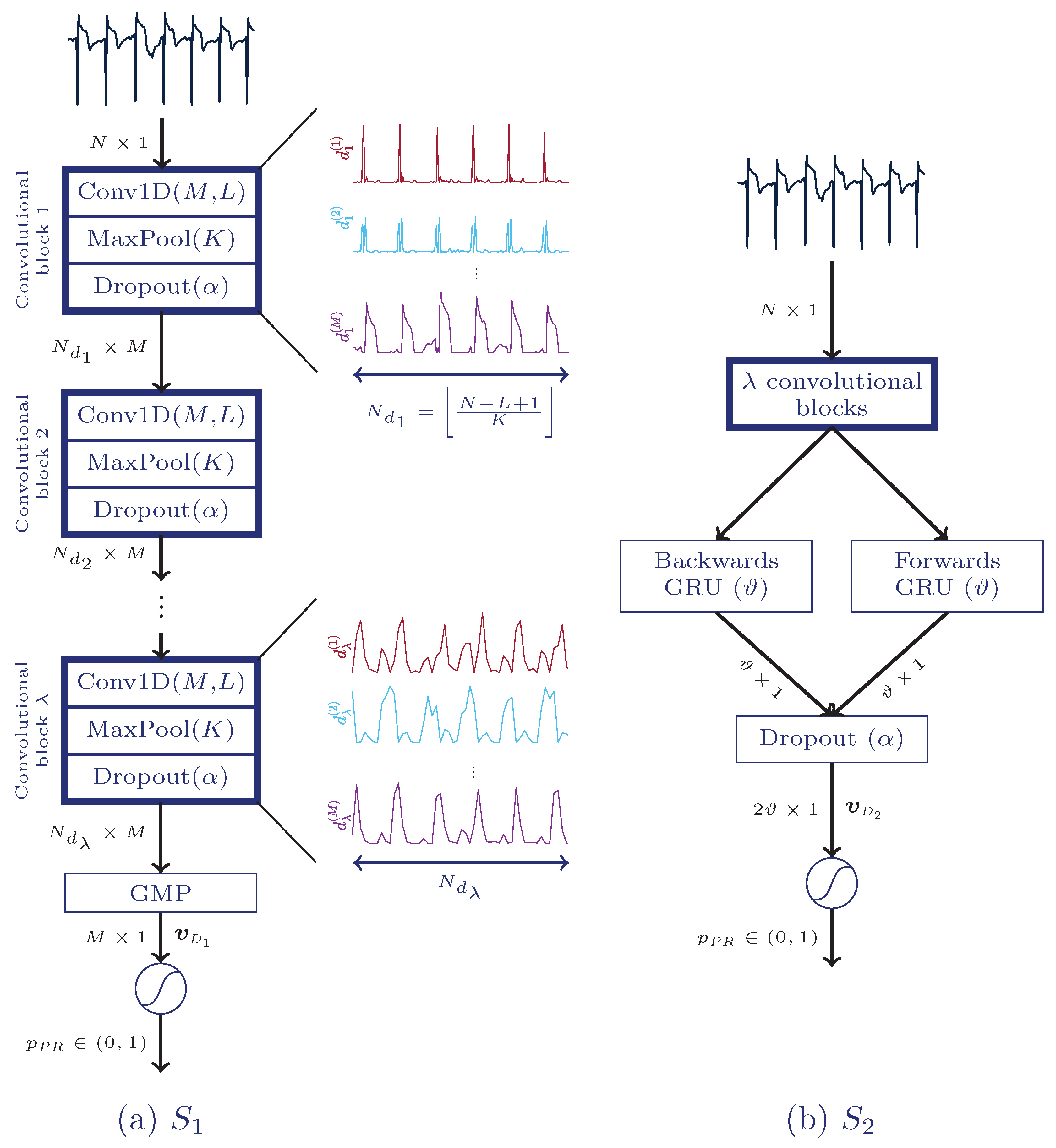
3.1. First Architecture: Fully Convolutional Neural Network

Panel a of Figure 2 shows the overall architecture of the first solution ($S_1$). It consists of $\lambda$ convolutional blocks, each one composed of a convolutional, a maximum pooling and a dropout layer.

Convolutional layers apply temporal convolution to the input signal. M different convolution kernels of size L allows obtaining M representations of the signal. The $\ell =1,\dots ,M$-th output for the input signal $s\left[n\right]$ is calculated as follows:

$$c_1^{(\ell )}\left[n\right]=\varphi \left(\sum _{i=0}^{L-1}{w}_i^{(\ell )}s[n-i]+b_i^{(\ell )}\right)$$

(1)

where w and b are the weights and biases, respectively, of the convolution kernel (adjusted during training) and $\varphi (·)$ is an activation function. The linear rectifier was adopted as activation function, i.e., $\varphi (·)=max\{0,·\}$. Since no padding was applied to $s\left[n\right]$ the length of $c_1^{(\ell )}\left[n\right]$ was $N_{c_1}=N-L+1$ (the first $L-1$ samples were discarded). The outputs of the first convolutional layer are fed into a max-pooling layer, which downsamples each input signal by applying the maximum operation with a pool size $K=2$ to non-overlapping signal segments:

$$p_1^{(\ell )}\left[n\right]=max{\left\{c_1^{(\ell )}\left[k\right]\right\}}_{k=(n-1)K+1}^{n·K}\mathrm{for}n=1,\dots ,⌊\frac{N_{c_1}}{K}⌋$$

(2)

The next step is to apply the dropout operation, which is only present during training and it is a common technique to avoid overfitting. It consists in dropping out some units under a certain probability $\alpha$ at each training step in a mini-batch. When some units are removed different networks are created at each step, so it can be seen as an ensemble technique. Let us denote the outputs of this layer as $d_1^{(\ell )}\left[n\right]$, which will have the same size as $p_1^{(\ell )}\left[n\right]$. Note that once the network is trained $d_1^{(\ell )}\left[n\right]=p_1^{(\ell )}\left[n\right]$.

Pooling layers remove redundant information and reduce the computational cost of the upper layers. The convolution operation of the network permits learning time-invariant features. We added more convolutional blocks with the same number of kernels M of size L. The outputs of the second convolutional layer are given by the following equation:

$$c_2^{(\ell )}\left[n\right]=\varphi \left(\sum _{j=1}^M\sum _{i=0}^{L-1}{w}_{ij}^{(\ell )}{d}_1^{\left(j\right)}[n-i]+b_{ij}^{(\ell )}\right)$$

(3)

These outputs are fed into another max-pooling and dropout layers to obtain $d_2^{(\ell )}\left[n\right]$, with M different representations of $N_{d_2}$ samples. The above equations can be easily adapted to obtain the outputs of the i-th convolutional block ($c_i^{(\ell )}$, $p_i^{(\ell )}$ and $d_i^{(\ell )}$) for $i=1,\dots ,\lambda$, where $\lambda$ is the number of convolutional blocks.

The next layer is another pooling layer, namely a global maximum pooling layer. Having M different representations of the signal the maximum value of each representation is adopted to obtain a feature vector of M elements, i.e.,

$${\mathit{v}}_{D_1}=max{\{d_{\lambda }^{(\ell )}\left[n\right]\}}_n\mathrm{for}\ell =1,\dots ,M$$

(4)

Finally, a fully connected layer was used as classification stage. This layer is composed of a single neuron with sigmoid activation function to produce $p_{PR}$:

$$p_{PR}=\frac{1}{1+e^{-(\mathit{w}·{\mathit{v}}_{{\mathrm{D}}_1}+\mathit{b})}}$$

(5)

According to [48], it is especially useful to train some layers of the network under the constraint $\left|\right|\mathit{w}\left|\right|<\gamma$ when using dropout. This additional constraint during the training process reduces overfitting, so every convolutional layer was trained with $\gamma =3.5$.

3.2. Second Architecture: CNN Combined with a Recurrent Layer

PEA and PR segments show different temporal behaviour. For instance, the time evolution for PR segments is known to be more regular than for PEA segments. These kind of temporal dynamics can be learned by a RNN. So the second solution proposed in this study ($S_2$) combines CNN and a bidirectional gated recurrent unit (BGRU), as shown in panel b of Figure 2.

GRU [49] is a simplified version of the well-known long short-term memory (LSTM) [50] with a similar performance [49]. These layers resolve long-term dependencies and avoid vanishing gradient problems. BGRU was inserted between the last convolutional block and the classification stage, removing the global maximum pooling layer. BGRU is composed of two GRU layers, one forward and the other one backward, so more sophisticated temporal features can be extracted by exploiting past and future information at time step n. Finally, both outputs were concatenated. A single GRU calculates hidden states ${\mathit{h}}_n$ at time step $n=1,\dots ,N_{d_{\lambda }}$ based on the past state. Given $\mathbf{D}=[d_{\lambda }^{\left(1\right)},\dots ,d_{\lambda }^{\left(M\right)}]$, the equations of the forwards GRU are described as follows:

$$\begin{array}{ccc}\hfill {\mathit{z}}_n& =& \sigma ({\mathbf{W}}_z\mathbf{D}+{\mathbf{U}}_z{\mathit{h}}_{n-1}+{\mathit{b}}_z)\hfill \end{array}$$

(6)

$$\begin{array}{ccc}\hfill {\mathit{r}}_n& =& \sigma ({\mathbf{W}}_r\mathbf{D}+{\mathbf{U}}_r{\mathit{h}}_{n-1}+{\mathit{b}}_r)\hfill \end{array}$$

(7)

$$\begin{array}{ccc}\hfill {\mathit{h}}_n^{\prime }& =& tanh(\mathbf{W}\mathbf{D}+{\mathbf{r}}_n\odot \mathbf{U}{\mathit{h}}_{n-1}+\mathit{b})\hfill \end{array}$$

(8)

$$\begin{array}{ccc}\hfill {\mathit{h}}_n& =& {\mathit{z}}_n\odot {\mathit{h}}_{n-1}+(1-{\mathit{z}}_n)\odot {\mathit{h}}_n^{\prime }\hfill \end{array}$$

(9)

where $\mathbf{W}$ and $\mathbf{U}$ are weight matrices, $\mathit{b}$ is the bias vector, $\sigma (•)$ stands for sigmoid function, and ⊙ is the Hadamard product. In the equations above ${\mathit{z}}_n$ and ${\mathit{r}}_n$ correspond to the update and reset gates, respectively. The backwards GRU works in the same way but the temporal representations of the input are flipped. The hidden state at the last time step, ${\mathit{h}}_{n=N_{d_{\lambda }}}$, is fed in to the next layer. Having $\vartheta$ units for each direction, a total of $2\vartheta$ features, ${\mathit{v}}_{\mathrm{D}}2=[v_{\mathrm{D}}{2}^{\left(1\right)},\dots ,v_{\mathrm{D}}{2}^{\left(2\vartheta \right)}]$, are fed to the last classification layer after applying dropout. The convolutional and recurrent layers were trained under the constraint $\left|\right|\mathit{w}\left|\right|<\gamma$.

Another kind of dropout in RNN is recurrent dropout [51], which affects the connections between recurrent units instead of the inputs/outputs of the layer. A recurrent dropout fraction of 0.15 was used to train the final model.

This architecture is optimized simultaneously to obtain the optimal representations of the signal (convolutional layers) and obtain the optimal temporal features (BGRU) for an artificial neural network classifier (fully connected layer).

3.3. Training Process

The weights and biases of every layer were optimized using the adaptive moment estimation (ADAM) optimizer [52]. ADAM is a stochastic gradient descent algorithm with adaptive learning rate. According to [52], good default settings are a learning rate of $0.001$ and exponential decay rates of $0.9$ and $0.999$.

The training data were fed into the DNN in batches of 8 during 75 epochs. At the beginning of each epoch training data were shuffled, so the mini-batches at each epoch were different. Additionally, zero-mean Gaussian noise with standard deviation of ${10}^{-4}$ was added to the signal, and its amplitude was modified by $\pm 2\%$ (uniformly distributed) at each mini-batch. This process enriches the generalization of the model, as the input data for each epoch differs slightly.

The cost function to minimize was the binary cross-entropy:

$$\mathcal{L}(p)=\sum _i{\eta }_i\left[y_i^{\left(true\right)}ln\left(p_{P{R}_i}\right)+(1-y_i^{\left(true\right)})ln(1-p_{P{R}_i})\right]$$

(10)

where $y^{\left(true\right)}=\{0:\mathrm{PEA},1:\mathrm{PR}\}$ are the manual annotations and ${\eta }_i$ are the sample weights. As patients contribute with different number of segments, every patient was weighted equally to train the DNN, so the sum of ${\eta }_i$ within the same patient is equal to 1.

Every experiment was carried out using Keras framework [53] with Tensorflow backend [54]. The DNNs were trained on an NVIDIA GeForce GTX 1080 Ti.

3.4. Uncertainty Estimation

The network’s output, $p_{PR}$, represents the likelihood of PR, but it is not an indicator of the prediction confidence of the model. The uncertainty of the DNN decision can be estimated using dropout and data augmentation also during the test phase, a procedure known as Monte–Carlo dropout [55]. For each segment of the test set the prediction is repeated N times but adding two random effects: dropout in the DNN network, and the addition of white noise to the ECG. This produces N values of $p_{PR}$, and the variance of those values is interpreted as the uncertainty of the prediction. In our experiments N was set to 100. The decisions in the test set with an uncertainty above an acceptable threshold were discarded, and in those cases feedback would not be given to the rescuer. The threshold of uncertainty is determined in the training set. The uncertainty of each training instance is computed and the threshold is determined as the uncertainty for which a proportion of feedbacks will be given. In our experiments we tested a proportion of feedbacks from 100% to 80%.

4. Baseline Approaches

Machine learning solutions based on well-known ECG features were implemented and compared with $S_1$ and $S_2$. A total of nine hand-crafted features proposed in [34], $\mathit{v}=[v^{\left(1\right)},\dots ,v^{\left(9\right)}]$, were computed. They quantify the PR/PEA differences in terms of QRS complex rate and narrowness, slope steepness, spectral energy distribution, and regularity of the signal (fuzzy entropy).

Three classifiers were optimized and trained:

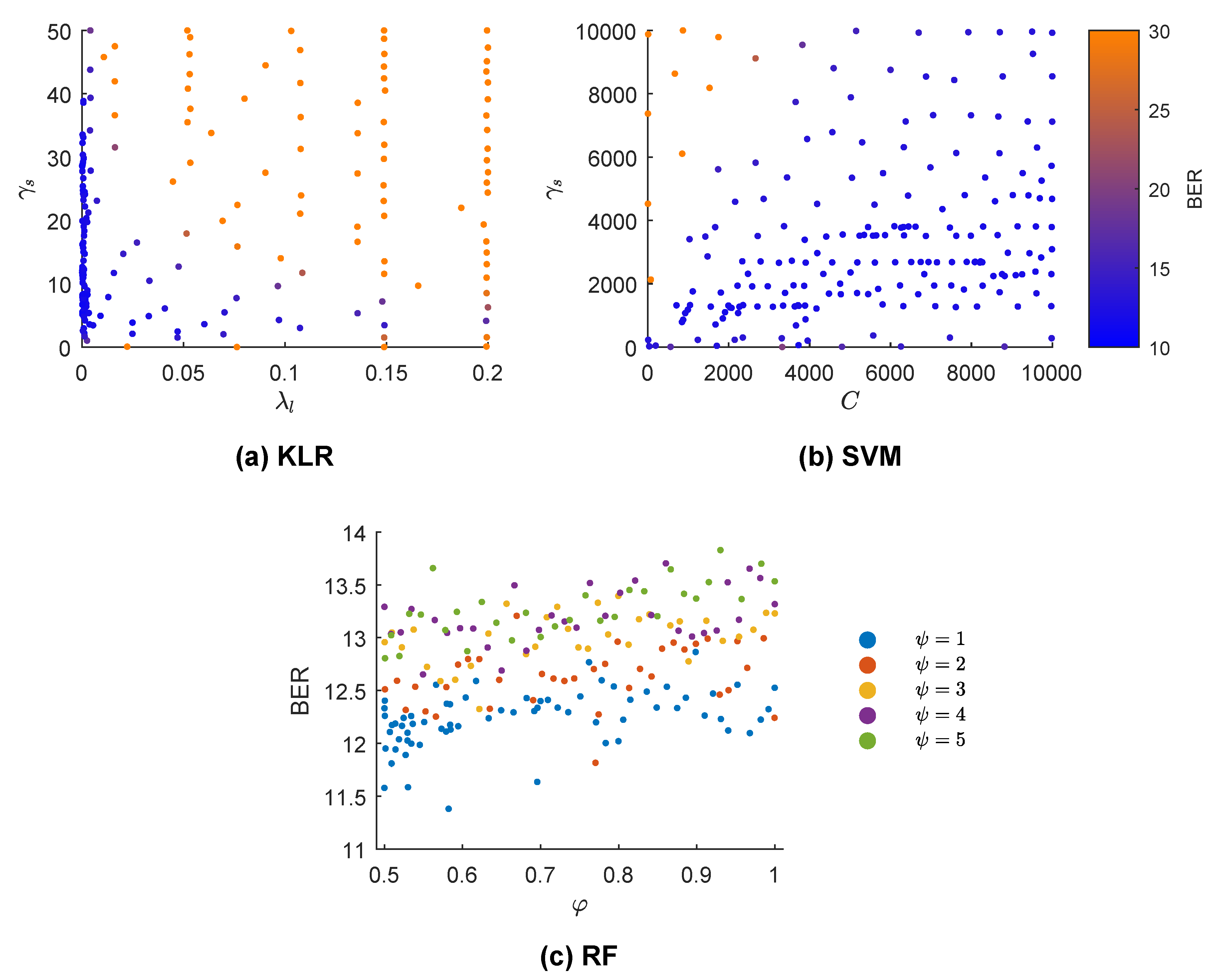
• RF: Introduced in [56], RF constructs many weak learners, each trained with a certain proportion of the training data, $\phi$. Each subset is generated by resampling with replacement. Each weak learner is a tree, and only $\psi$ features are considered (drawn randomly from an uniform distribution) at each node. The final decision is made by majority voting. We set the number of trees to 300, and optimized the hyper-parameters $\phi$ and $\psi$.
• Support vector machine (SVM): Given a feature vector $\mathit{v}$, the SVM makes the prediction using the following formula [57]:

  $$y^{\left(pred\right)}=\mathrm{sign}\left(b+\sum _{i=1}^{N_s}{w}_{i}K(\mathit{v},{\mathit{v}}_{\mathit{i}})\right)$$

  (11)

  where b is the intercept term and $N_s$ is the number of support vectors ($w_i$ is non-zero only for these vectors). Here $K(·,·)$ denotes the kernel function, which for a Gaussian kernel with ${\gamma }_s$ width is:

  $$K(\mathit{v},{\mathit{v}}_{\mathit{i}})=exp(-{\gamma }_s\left|\right|\mathit{v}-{\mathit{v}}_{\mathit{i}}{\left|\right|}^2)$$

  (12)

  The hyper-parameters soft margin C and ${\gamma }_s$ were optimized for the SVM.
• Kernel logistic regression (KLR): This is a version of the well-known logistic regression by applying a kernel-trick [57,58]. The prediction is made using Equation (11), and the kernel of Equation (12). The hyper-parameters to optimize were the regularization-term ${\lambda }_l$ and ${\gamma }_s$.

5. Evaluation Setup and Optimization Process

5.1. Evaluation Setup

The performance of the models was evaluated in terms of sensitivity (Se, probability of correctly identifying PR), specificity (Sp, probability of correctly identifying PEA), and balanced accuracy (BAC, arithmetic mean between Se and Sp). The balanced error rate (BER) was defined as $1-\mathrm{BAC}$. As patients have different numbers of segments, every patient was weighted equally to compute the performance metrics.

5.2. Hyper-Parameter Optimization Process

The hyper-parameters of every model were optimized using Bayesian optimization (BO) [59]. BO is a probabilistic model based approach that attempts to minimize an objective function associated with a real-valued metric, and the variables to optimize can be discrete or continuous. Recent studies report that BO is more efficient than grid search, random search, or manual tuning since it requires less time and the overall performance on the test set is better [60].

BO approximates the objective function to a surrogate function that is cheaper to evaluate. At each iteration a candidate solution is tested to update the surrogate using the past information. With more iterations the approximation of the surrogate is better. BO algorithm variants differ on how this surrogate is constructed. In this study we considered tree-structured parzen estimators (BO-TPE, to optimize $S_1$ and $S_2$) and Gaussian processes (BO-GP, to optimize RF, SVM, and KLR) [60,61].

The training data were divided patient-wise into 4 folds, and the cross-validated BER was the objective function to minimize. The search space for all models is shown in

Table 1. Search space of Bayesian optimization (BO) for all models. Here $\mathcal{U}(\min ,\max )$ denotes a uniform distribution between min and max values.

Model	Hyper-Parameters
RF	$\vartheta =\mathcal{U}(0.5,1)$
	$\psi =\{1,\dots ,9\}$
SVM	$C=\mathcal{U}$(0.001, 10,000)
	${\gamma }_s=\mathcal{U}$(0.001, 10,000)
KLR	${\lambda }_l=\mathcal{U}(0.0001,0.2)$
	${\gamma }_s=\mathcal{U}(0.0001,15)$
$S_1$	$\lambda =\{1,2,3,4,5\}$
	$M=\{8,16,24\}$
	$L=\{5,6,7,8\}$
	$\alpha =\mathcal{U}(0.05,0.5)$
$S_2$	$\lambda =\{1,2,3,4,5\}$
	$M=\{8,16,24\}$
	$L=\{5,6,7,8\}$
	$\alpha =\mathcal{U}(0.05,0.5)$
	$\vartheta =\{4,5,6,7,8\}$

.

6. Results

The results of the BO-TPE algorithm applied for $S_1$ are shown in Figure 3. For each hyper-parameter the values of the cross-validated BER are given, continuous for $\alpha$ and median (10–90 percentiles) for the other discrete hyper-parameters. The distributions of the values selected by the optimizing algorithm are also shown (as histogram for $\alpha$). The number of convolutional blocks, $\lambda$, and the dropout rate, $\alpha$, turned out very determinant. Values of $\alpha >0.3$ rapidly increased the BER, and including up to $\lambda =4$ blocks was the most selected option by the optimization algorithm. The values of M and L in the selected range had small effect on the performance of the classifier.

Figure 4 shows the results of BO-TPE for $S_2$. Increasing $\lambda$ overfitted the model rapidly and BER was minimum for $\lambda =2$; less convolutional blocks did not provide detailed enough features and increasing $\lambda$ overfitted the model. Another influential hyper-parameter was $\alpha$, which showed minimum BER values around $0.4$. The hyper-parameters M, L, and $\vartheta$ had little effect on BER.

Figure 5 shows the results of the BO-GP algorithm applied to tune the hyper-parameters of the KLR, SVM, and RF models. The cross-validated BER is color-coded (KLR and SVM) or depicted in the vertical axis (RF). Each point shows a single hyper-parameter combination tested by the BO-GP. In the case of KLR, both hyper-parameters were important, but low values of ${\lambda }_l$ especially yielded lower BER values. For the SVM, low values of C and high values of ${\gamma }_s$ produced the worst results, but the selection in the range of values was not as critical as in the KLR solution. Lastly, for RF $\psi =1$ was the best option, particularly for $0.5<\phi <0.6$, although the fine tuning of $\phi$ was not critical.

Table 2. Summary of the performance of the deep learners and baseline models with the test set and the optimal hyper-parameters chosen by the Bayesian optimization with Gaussian processes (BO-GP) and Bayesian optimization with tree-structured parzen estimators (BO-TPE) algorithms with 5-s electrocardiogram (ECG) segments. DNN models outperformed baseline models in terms of BAC.

	Se (%)	Sp (%)	BAC (%)	Hyper-Parameters
Baseline models
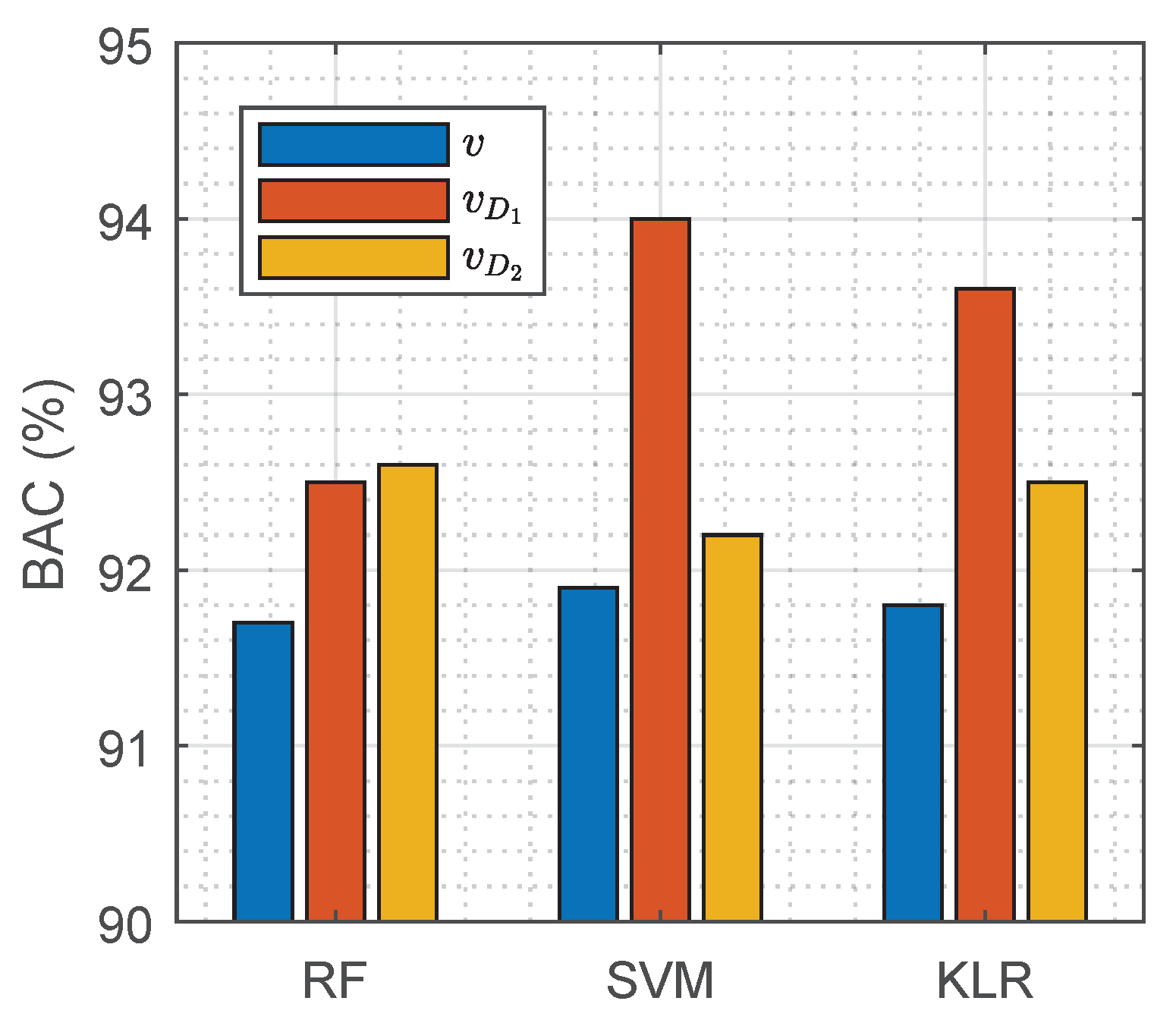
RF	96.0	87.4	91.7	$\{\phi ,\psi \}=\{0.58,1\}$
SVM	97.6	86.2	91.9	$\{C,{\gamma }_s\}=\{2038,1246\}$
KLR	97.5	86.2	91.8	$\{{\lambda }_l,{\gamma }_s\}=\{0.0013,7\}$
DNN models
$S_1$	94.1	92.9	93.5	$\{\lambda ,M,L,\alpha \}=\{4,8,7,0.2\}$
$S_2$	95.5	91.6	93.5	$\{\lambda ,M,L,\alpha ,\vartheta \}=\{2,24,6,0.4,6\}$

shows the overall test results of the baseline models and the deep learners in terms of Se, Sp, and BAC, and the set of selected hyper-parameters tuned during the optimization process. There were no differences between the RF, SVM, and KLR models, and any of the deep learning solutions outperformed the baseline models by nearly two percentage points of BAC. Although there was no difference in performance between $S_1$ and $S_2$, the training process of $S_1$ is simpler with less trainable parameters than $S_2$ (1441 vs. 4777).

In

Table 3. Computation time to classify a 5-s segment for the baseline and deep neural network (DNN) models. The fastest model was $S_1$.

	${\mathit{t}}_1$ (ms)	${\mathit{t}}_2$ (ms)	Total (ms)
Baseline models
RF	63.5	0.28	63.8
SVM	63.5	0.35	63.9
KLR	63.5	0.25	63.8
DNN models
$S_1$	-	-	1.6
$S_2$	-	-	101.1

the computation time of the different models is compared. The mean time required to classify the 5 s segment is given, separately for the baseline classifiers in terms of required time for feature extraction ($t_1$) and classification ($t_2$). Processing times were calculated on a single core of an Intel Xeon 3.6 GHz. As shown in Table 3 the fully convolutional solution, $S_1$, was by far the fastest one followed by the baseline models.

Comparative analyses were performed between the 9 hand-crafted features of the baseline models ($\mathit{v}$) and the features learnt by DNN solutions $S_1$ and $S_2$ (${\mathit{v}}_{D_1}$ and ${\mathit{v}}_{D_2}$ respectively). The area under the curve (AUC) for $\mathit{v}$ ranged between 0.88 and 0.94, showing that they had been wisely selected in different domains as described in [34]; but the $M=8$ features (${\mathit{v}}_{D_1}$) that $S_1$ extracted reported high discriminative values from 0.61 to 0.97, showing that the deep architecture found some very selective features. Next, feature sets from the deep learners ${\mathit{v}}_{D_1}$ and ${\mathit{v}}_{D_2}$ were fed into the baseline classifiers to compare their performance with that of the original $\mathit{v}$. The BO-GP optimization procedure was repeated for the RF, SVM, and KLR classifiers and results for the test set are depicted in Figure 6. Training the classifiers with ${\mathit{v}}_{D_1}$ and ${\mathit{v}}_{D_2}$ yielded higher BAC values than those obtained with the pre-designed $\mathit{v}$ features. This experiment shows that features defined by the neural networks integrate information not considered by the hand-crafted features, and that they can be successfully used with other classifiers.

The duration of the ECG segment fed into any of the solutions is critical when using a pulse detection algorithm during OHCA treatment. During CPR the ECG signal is strongly affected by chest compression artefacts and electrical defibrillation attempts. For any diagnosis based on the ECG, intervals free of artefact must be used, i.e., extracted either during pauses for rhythm analysis or during chest compression pauses. The segment length used in this study is below the typical interruption for a rhythm analysis, which is between 5.2–26.3 s [62]. However, decreasing the length of the analysis segment would contribute to shorter interruptions in compressions for pulse detection. Reducing hands-off intervals that compromise oxygen delivery to the vital organs increases survival rates [63,64]. Consequently, the solutions of this proposal were tested for different segment durations, from 5 s down to 2 s. The models that were trained for 5-s ECG segments were used, features were extracted using the first seconds of the segment, and those features were fed into the baseline models. The DNN models were fed with the same first seconds of the ECG segments used for feature calculation (note that $S_1$ and $S_2$ can work with any segment duration at the input). As shown in Figure 7 the best performance for the baseline models was obtained for segment lengths of 5 s. The DNN models outperformed the best baseline models for any segment length, including segments as short as 2 s.

A last evaluation of $S_1$ was performed to assess the influence of the degree of uncertainty in the decision of the model.

Table 4. Performance of $S_1$ with different degrees of uncertainty. Scores are given for the test set and the percentage of feedback in the test set are reported. The threshold for feedback was set in the training set.

Training Percentage	Testing Percentage	Se (%)	Sp (%)	BAC (%)
80	78.5	100	95.2	97.6
90	89.6	96.6	93.2	94.9
95	95.4	97.1	92.2	94.6
97.5	98.1	96.3	92.1	94.2
100	100	94.1	92.9	93.5

shows the performance of the model if the system was designed to give feedback only in a percentage of the analyses, those in which the uncertainty of the decision was lowest. Different percentage thresholds were tested in the training set, from 100% (always give feedback) to 80% (give feedback when the uncertainty is low). Assuming no feedback in 5% of the cases increased the BAC by one percentage point, and the BAC increased up to 97.6% if the system was designed to discard the 20% of the analyses with largest uncertainty.

7. Discussion and Conclusions

Pulse detection during OHCA is still an unsolved problem, and there is a need for automatic methods to assist the rescuer (bystander or medical personnel) to decide whether the patient has pulse or not [10]. Non-invasive pulse detection is still a challenging problem [16], and no solutions are currently integrated in monitors/defibrillators. To the best of our knowledge, this is the first study that uses DNN models to discriminate between PR and PEA rhythms using exclusively the ECG.

The two DNN models proposed in this study outperformed the best PR/PEA discriminators based exclusively on the ECG published to date. A RF classifier based on hand-crafted features was proposed in [34] and reported Se/Sp of 88.4%/89.7% for a smaller dataset. A DNN model using a single convolutional layer followed by a recurrent layer was introduced in a conference paper [65], but the Se/Sp/BAC were 91.7%/92.5%/92.1% on the dataset used for this study, that is the BAC was 1.5 percentage points below the current solution. Other DNN solutions were tested in another conference paper [66], where we reported BAC values of 91.2% and 92.6% for preliminary versions of $S_1$ and $S_2$. Performance was improved in this study adding a general DNN architecture with multiple convolutional layers, a Bayesian optimization procedure which provided insights into the critical hyper-parameters of the networks (see Figure 3 and Figure 4), and a better data augmentation procedure. All these factors contributed to an improved BAC of 93.5% for $S_1$ and $S_2$, an increase of nearly 2 points from a baseline BAC around 92%, i.e., achieving 20% of the available margin for improvement (8 points) on our initial architectures. Furthermore, we also introduced a new usage framework in which the algorithm was able to automatically assess the uncertainty of the decision, and improved feedback by only reporting decisions with low uncertainties.

There was no difference in terms of BAC between $S_1$ and $S_2$. The second solution is more complex and should be able to capture more sophisticated features of the signal. However, the number of trainable parameters was 1441 in $S_1$ and 4777 in $S_2$. Increasing the number of trainable parameters makes the DNN model prone to overfitting, the model “memorizes” the training data loosing generalization capacity and shows poorer performance with unseen data [67,68]. In fact, $S_2$ showed higher accuracies during training than $S_1$ ($98.5\%$ vs. $96.6\%$). Besides, training was computationally more costly for $S_2$, optimizing $S_1$ required $\approx 37$ h and optimizing $S_2$$\approx 82$ h. However, it is possible that with larger datasets $S_2$ could generalize better and provide a more accurate model, but OHCA datasets with pulse annotations are costly.

DNN architectures are capable of automatically learning the discrimination features. Our results show that the features learned by $S_1$ and $S_2$ produced more accurate PR/PEA classifiers than hand-crafted features when fed to the classical machine learning models (see Figure 6). The DNN architectures were able to capture some important ECG characteristics for the identification of pulse that are not accounted for in the hand-crafted features proposed in the literature. In particular, the most discriminative features were those learned by $S_1$, which when fed to an SVM classifier boosted the BAC from 92% for hand-crafted features to above 94%.

One of the salient features of the proposed DNN solutions is that they are based solely on the ECG. The ECG is available in all defibrillators/monitors used to treat OHCA patients, so it could be integrated into any equipment. PR/PEA discrimination algorithms that use the ECG and TI have also been proposed [28,29], the TI adds relevant information because effective heartbeats may produce small fluctuations in the TI [23,24]. The BACs of ECG/TI-based PR/PEA discriminators using classical machine learning approaches were around 92% for smaller datasets [28,29]. Defibrillators measure the impedance to check that pads are properly attached to the patient’s chest, that is the reason why the TI signal is not recorded with m$\mathsf{\Omega }$ amplitude resolution in many devices. In any case, multi-modal deep learning solutions could be explored to increase the accuracy by designing DNN solutions that use both the ECG and TI signals. Moreover, $S_1$ extracted significant features, so it could be used as a feature extractor and those features could be combined with features derived from the TI, and other surrogate measures of the hemodynamic state of the patient.

Another critical factor of automatic PR/PEA discrimination algorithms is the ECG segment length needed for an accurate decision. PR/PEA discrimination algorithms need an ECG without chest compression artefacts, this means that compressions have to be interrupted for pulse detection. Pauses in chest compressions compromise the survival of the patient [63,64]. Therefore, current guidelines recommend interruptions of less than 10 s for pulse checks [4,10], but in practice these interruptions are longer than 10 s in more than 50% of cases [14,15]. Our DNN models were very accurate for a segment length of 5 s. Moreover, the length of the segment could be shortened down to 2 s without compromising the BAC of our models (see Figure 7). Consequently, our automatic algorithm could be used to reliably detect pulse during OHCA with interruptions as short as 2–3 seconds, and could be used to avoid the excessively long pauses in chest compressions for pulse detection observed during OHCA treatment.

Measuring the uncertainty of the prediction may be useful when misclassifying an input has a considerable cost, for instance a false pulse indication may unnecessarily interrupt a life saving therapy like CPR. Many efforts have been made to estimate the uncertainty in DNN models, but it is still a challenging problem [69,70,71,72,73]. In this work the uncertainty of the decision was measured using a method known as Monte–Carlo dropout [55], and we found that only giving feedback when the uncertainty was low considerably increased the BAC. For instance, giving a feedback in the 95% of the cases improved the BAC by more than 1 point, and only giving feedback in 80% of cases increased the BAC by over 4 points. During OHCA treatment CPR should be continued until a reliable pulse detection is identified by the algorithm, and the pauses in compressions for the potential feedbacks (reliable or unreliable) will be short, since our algorithms only require ECG segments of 2–3 s. Further work should be done to improve the estimate of the uncertainty of the decision, so that BACs of 97% could be obtained by discarding less than 20% of the potential feedbacks.

In conclusion, this study introduces the use of deep neural networks to discriminate between pulseless and pulsatile rhythms during OHCA using only the ECG. The proposed DNN models outperformed hand-crafted feature-based machine learning solutions, and were able to accurately detect pulse with ECG segments as short as 2–3 s. Moreover, a first attempt at a quantification of the uncertainty of the decision was also introduced to improve the reliability of the feedback given to the rescuer. The proposed solution is based exclusively on the ECG and could be integrated into any monitor/defibrillator.

References

- Gräsner, J.T.; Bossaert, L. Epidemiology and management of cardiac arrest: What registries are revealing. Best Pract. Res. Clin. Anaesthesiol. 2013, 27, 293–306. [Google Scholar] [CrossRef] [PubMed]
- Berdowski, J.; Berg, R.A.; Tijssen, J.G.; Koster, R.W. Global incidences of out-of-hospital cardiac arrest and survival rates: Systematic review of 67 prospective studies. Resuscitation 2010, 81, 1479–1487. [Google Scholar] [CrossRef] [PubMed]
- Deakin, C.D. The chain of survival: Not all links are equal. Resuscitation 2018, 126, 80–82. [Google Scholar] [CrossRef] [PubMed]
- Perkins, G.D.; Handley, A.J.; Koster, R.W.; Castrén, M.; Smyth, M.A.; Olasveengen, T.; Monsieurs, K.G.; Raffay, V.; Gräsner, J.T.; Wenzel, V.; et al. European Resuscitation Council Guidelines for Resuscitation 2015: Section 2. Adult basic life support and automated external defibrillation. Resuscitation 2015, 95, 81–99. [Google Scholar] [CrossRef] [PubMed]
- Bahr, J.; Klingler, H.; Panzer, W.; Rode, H.; Kettler, D. Skills of lay people in checking the carotid pulse. Resuscitation 1997, 35, 23–26. [Google Scholar] [CrossRef]
- Eberle, B.; Dick, W.; Schneider, T.; Wisser, G.; Doetsch, S.; Tzanova, I. Checking the carotid pulse check: Diagnostic accuracy of first responders in patients with and without a pulse. Resuscitation 1996, 33, 107–116. [Google Scholar] [CrossRef]
- Ochoa, F.J.; Ramalle-Gomara, E.; Carpintero, J.; Garcıa, A.; Saralegui, I. Competence of health professionals to check the carotid pulse. Resuscitation 1998, 37, 173–175. [Google Scholar] [CrossRef]
- Lapostolle, F.; Le Toumelin, P.; Agostinucci, J.M.; Catineau, J.; Adnet, F. Basic cardiac life support providers checking the carotid pulse: Performance, degree of conviction, and influencing factors. Acad. Emerg. Med. 2004, 11, 878–880. [Google Scholar] [CrossRef]
- Tibballs, J.; Russell, P. Reliability of pulse palpation by healthcare personnel to diagnose paediatric cardiac arrest. Resuscitation 2009, 80, 61–64. [Google Scholar] [CrossRef] [PubMed]
- Soar, J.; Nolan, J.; Böttiger, B.; Perkins, G.; Lott, C.; Carli, P.; Pellis, T.; Sandroni, C.; Skrifvars, M.; Smith, G.; et al. Section 3. Adult advanced life support: European Resuscitation Council Guidelines for Resuscitation 2015. Resuscitation 2015, 95, 100–147. [Google Scholar] [CrossRef]
- Ruppert, M.; Reith, M.W.; Widmann, J.H.; Lackner, C.K.; Kerkmann, R.; Schweiberer, L.; Peter, K. Checking for breathing: Evaluation of the diagnostic capability of emergency medical services personnel, physicians, medical students, and medical laypersons. Ann. Emerg. Med. 1999, 34, 720–729. [Google Scholar] [CrossRef]
- Perkins, G.D.; Stephenson, B.; Hulme, J.; Monsieurs, K.G. Birmingham assessment of breathing study (BABS). Resuscitation 2005, 64, 109–113. [Google Scholar] [CrossRef]
- Zengin, S.; Gümüşboğa, H.; Sabak, M.; Eren, Ş.H.; Altunbas, G.; Al, B. Comparison of manual pulse palpation, cardiac ultrasonography and Doppler ultrasonography to check the pulse in cardiopulmonary arrest patients. Resuscitation 2018, 133, 59–64. [Google Scholar] [CrossRef] [PubMed]
- Clattenburg, E.J.; Wroe, P.; Brown, S.; Gardner, K.; Losonczy, L.; Singh, A.; Nagdev, A. Point-of-care ultrasound use in patients with cardiac arrest is associated prolonged cardiopulmonary resuscitation pauses: A prospective cohort study. Resuscitation 2018, 122, 65–68. [Google Scholar] [CrossRef]
- in’t Veld, M.A.H.; Allison, M.G.; Bostick, D.S.; Fisher, K.R.; Goloubeva, O.G.; Witting, M.D.; Winters, M.E. Ultrasound use during cardiopulmonary resuscitation is associated with delays in chest compressions. Resuscitation 2017, 119, 95–98. [Google Scholar] [CrossRef] [PubMed]
- Babbs, C.F. We still need a real-time hemodynamic monitor for CPR. Resuscitation 2013, 84, 1297–1298. [Google Scholar] [CrossRef]
- Irusta, U.; Ruiz, J.; Aramendi, E.; de Gauna, S.R.; Ayala, U.; Alonso, E. A high-temporal resolution algorithm to discriminate shockable from nonshockable rhythms in adults and children. Resuscitation 2012, 83, 1090–1097. [Google Scholar] [CrossRef] [PubMed]
- Figuera, C.; Irusta, U.; Morgado, E.; Aramendi, E.; Ayala, U.; Wik, L.; Kramer-Johansen, J.; Eftestøl, T.; Alonso-Atienza, F. Machine learning techniques for the detection of shockable rhythms in automated external defibrillators. PLoS ONE 2016, 11, e0159654. [Google Scholar] [CrossRef]
- Li, Q.; Rajagopalan, C.; Clifford, G.D. Ventricular fibrillation and tachycardia classification using a machine learning approach. IEEE Trans. Biomed. Eng. 2014, 61, 1607–1613. [Google Scholar] [PubMed]
- Jekova, I.; Krasteva, V. Real time detection of ventricular fibrillation and tachycardia. Physiol. Meas. 2004, 25, 1167. [Google Scholar] [CrossRef] [PubMed]
- Myerburg, R.J.; Halperin, H.; Egan, D.A.; Boineau, R.; Chugh, S.S.; Gillis, A.M.; Goldhaber, J.I.; Lathrop, D.A.; Liu, P.; Niemann, J.T.; et al. Pulseless electric activity: Definition, causes, mechanisms, management, and research priorities for the next decade: Report from a National Heart, Lung, and Blood Institute workshop. Circulation 2013, 128, 2532–2541. [Google Scholar] [CrossRef] [PubMed]
- Ayala, U.; Irusta, U.; Ruiz, J.; Eftestøl, T.; Kramer-Johansen, J.; Alonso-Atienza, F.; Alonso, E.; González-Otero, D. A reliable method for rhythm analysis during cardiopulmonary resuscitation. BioMed Res. Int. 2014, 2014, 872470. [Google Scholar] [CrossRef] [PubMed]
- Johnston, P.; Imam, Z.; Dempsey, G.; Anderson, J.; Adgey, A. The transthoracic impedance cardiogram is a potential haemodynamic sensor for an automated external defibrillator. Eur. Heart J. 1998, 19, 1879–1888. [Google Scholar] [CrossRef] [Green Version]
- Pellis, T.; Bisera, J.; Tang, W.; Weil, M.H. Expanding automatic external defibrillators to include automated detection of cardiac, respiratory, and cardiorespiratory arrest. Crit. Care Med. 2002, 30, S176–S178. [Google Scholar] [CrossRef] [PubMed]
- Losert, H.; Risdal, M.; Sterz, F.; Nysæther, J.; Köhler, K.; Eftestøl, T.; Wandaller, C.; Myklebust, H.; Uray, T.; Aase, S.O.; et al. Thoracic-impedance changes measured via defibrillator pads can monitor signs of circulation. Resuscitation 2007, 73, 221–228. [Google Scholar] [CrossRef]
- Cromie, N.A.; Allen, J.D.; Turner, C.; Anderson, J.M.; Adgey, A.A.J. The impedance cardiogram recorded through two electrocardiogram/defibrillator pads as a determinant of cardiac arrest during experimental studies. Crit. Care Med. 2008, 36, 1578–1584. [Google Scholar] [CrossRef]
- Cromie, N.A.; Allen, J.D.; Navarro, C.; Turner, C.; Anderson, J.M.; Adgey, A.A.J. Assessment of the impedance cardiogram recorded by an automated external defibrillator during clinical cardiac arrest. Crit. Care Med. 2010, 38, 510–517. [Google Scholar] [CrossRef]
- Risdal, M.; Aase, S.O.; Kramer-Johansen, J.; Eftesol, T. Automatic identification of return of spontaneous circulation during cardiopulmonary resuscitation. IEEE Trans. Biomed. Eng. 2008, 55, 60–68. [Google Scholar] [CrossRef]
- Alonso, E.; Aramendi, E.; Daya, M.; Irusta, U.; Chicote, B.; Russell, J.K.; Tereshchenko, L.G. Circulation detection using the electrocardiogram and the thoracic impedance acquired by defibrillation pads. Resuscitation 2016, 99, 56–62. [Google Scholar] [CrossRef]
- Lee, Y.; Shin, H.; Choi, H.J.; Kim, C. Can pulse check by the photoplethysmography sensor on a smart watch replace carotid artery palpation during cardiopulmonary resuscitation in cardiac arrest patients? a prospective observational diagnostic accuracy study. BMJ Open 2019, 9. [Google Scholar] [CrossRef]
- Wijshoff, R.W.; van Asten, A.M.; Peeters, W.H.; Bezemer, R.; Noordergraaf, G.J.; Mischi, M.; Aarts, R.M. Photoplethysmography-based algorithm for detection of cardiogenic output during cardiopulmonary resuscitation. IEEE Trans. Biomed. Eng. 2015, 62, 909–921. [Google Scholar] [CrossRef] [PubMed]
- Brinkrolf, P.; Borowski, M.; Metelmann, C.; Lukas, R.P.; Pidde-Küllenberg, L.; Bohn, A. Predicting ROSC in out-of-hospital cardiac arrest using expiratory carbon dioxide concentration: Is trend-detection instead of absolute threshold values the key? Resuscitation 2018, 122, 19–24. [Google Scholar] [CrossRef]
- Wei, L.; Chen, G.; Yang, Z.; Yu, T.; Quan, W.; Li, Y. Detection of spontaneous pulse using the acceleration signals acquired from CPR feedback sensor in a porcine model of cardiac arrest. PLoS ONE 2017, 12, e0189217. [Google Scholar] [CrossRef] [PubMed]
- Elola, A.; Aramendi, E.; Irusta, U.; Del Ser, J.; Alonso, E.; Daya, M. ECG-based pulse detection during cardiac arrest using random forest classifier. Med. Biol. Eng. Comput. 2019, 57, 453–462. [Google Scholar] [CrossRef] [PubMed]
- Faust, O.; Hagiwara, Y.; Hong, T.J.; Lih, O.S.; Acharya, U.R. Deep learning for healthcare applications based on physiological signals: A review. Comput. Methods Programs Biomed. 2018, 161, 1–13. [Google Scholar] [CrossRef]
- Shen, S.; Yang, H.; Li, J.; Xu, G.; Sheng, M. Auditory Inspired Convolutional Neural Networks for Ship Type Classification with Raw Hydrophone Data. Entropy 2018, 20, 990. [Google Scholar] [CrossRef]
- Almgren, K.; Krishna, M.; Aljanobi, F.; Lee, J. AD or Non-AD: A Deep Learning Approach to Detect Advertisements from Magazines. Entropy 2018, 20, 982. [Google Scholar] [CrossRef]
- Cohen, I.; David, E.O.; Netanyahu, N.S. Supervised and Unsupervised End-to-End Deep Learning for Gene Ontology Classification of Neural In Situ Hybridization Images. Entropy 2019, 21, 221. [Google Scholar] [CrossRef]
- Al Rahhal, M.M.; Bazi, Y.; Al Zuair, M.; Othman, E.; BenJdira, B. Convolutional neural networks for electrocardiogram classification. J. Med. Biol. Eng. 2018, 38, 1014–1025. [Google Scholar] [CrossRef]
- Kiranyaz, S.; Ince, T.; Gabbouj, M. Real-time patient-specific ECG classification by 1-D convolutional neural networks. IEEE Trans. Biomed. Eng. 2016, 63, 664–675. [Google Scholar] [CrossRef]
- Acharya, U.R.; Fujita, H.; Lih, O.S.; Hagiwara, Y.; Tan, J.H.; Adam, M. Automated detection of arrhythmias using different intervals of tachycardia ECG segments with convolutional neural network. Inf. Sci. 2017, 405, 81–90. [Google Scholar] [CrossRef]
- Xia, Y.; Wulan, N.; Wang, K.; Zhang, H. Detecting atrial fibrillation by deep convolutional neural networks. Comput. Biol. Med. 2018, 93, 84–92. [Google Scholar] [CrossRef]
- Acharya, U.R.; Fujita, H.; Oh, S.L.; Hagiwara, Y.; Tan, J.H.; Adam, M. Application of deep convolutional neural network for automated detection of myocardial infarction using ECG signals. Inf. Sci. 2017, 415, 190–198. [Google Scholar] [CrossRef]
- Lipton, Z.C.; Kale, D.C.; Elkan, C.; Wetzel, R. Learning to diagnose with LSTM recurrent neural networks. arXiv, 2015; arXiv:1511.03677. [Google Scholar]
- Chauhan, S.; Vig, L. Anomaly detection in ECG time signals via deep long short-term memory networks. In Proceedings of the 2015 IEEE International Conference on Data Science and Advanced Analytics (DSAA), Paris, France, 19–21 October 2015; pp. 1–7. [Google Scholar]
- Alonso, E.; Ruiz, J.; Aramendi, E.; González-Otero, D.; de Gauna, S.R.; Ayala, U.; Russell, J.K.; Daya, M. Reliability and accuracy of the thoracic impedance signal for measuring cardiopulmonary resuscitation quality metrics. Resuscitation 2015, 88, 28–34. [Google Scholar] [CrossRef]
- Ayala, U.; Eftestøl, T.; Alonso, E.; Irusta, U.; Aramendi, E.; Wali, S.; Kramer-Johansen, J. Automatic detection of chest compressions for the assessment of CPR-quality parameters. Resuscitation 2014, 85, 957–963. [Google Scholar] [CrossRef]
- Srivastava, N.; Hinton, G.; Krizhevsky, A.; Sutskever, I.; Salakhutdinov, R. Dropout: A simple way to prevent neural networks from overfitting. J. Mach. Learn. Res. 2014, 15, 1929–1958. [Google Scholar]
- Chung, J.; Gulcehre, C.; Cho, K.; Bengio, Y. Empirical evaluation of gated recurrent neural networks on sequence modeling. arXiv, 2014; arXiv:1412.3555. [Google Scholar]
- Hochreiter, S.; Schmidhuber, J. Long short-term memory. Neural Comput. 1997, 9, 1735–1780. [Google Scholar] [CrossRef]
- Gal, Y.; Ghahramani, Z. A theoretically grounded application of dropout in recurrent neural networks. Adv. Neural Inf. Process. Syst. 2016, 1019–1027. [Google Scholar]
- Kingma, D.P.; Ba, J. Adam: A method for stochastic optimization. arXiv, 2014; arXiv:1412.6980. [Google Scholar]
- Chollet, F. Keras-Team/keras. Available online: https://github.com/fchollet/keras (accessed on 20 March 2019).
- Abadi, M.; Agarwal, A.; Barham, P.; Brevdo, E.; Chen, Z.; Citro, C.; Corrado, G.S.; Davis, A.; Dean, J.; Devin, M.; et al. TensorFlow: Large-Scale Machine Learning on Heterogeneous Systems. 2015. Available online: tensorflow.org (accessed on 20 March 2019).
- Gal, Y.; Ghahramani, Z. Dropout as a bayesian approximation: Representing model uncertainty in deep learning. In Proceedings of the International Conference on Machine Learning, New York, NY, USA, 19–24 June 2016; pp. 1050–1059. [Google Scholar]
- Breiman, L. Random forests. Mach. Learn. 2001, 45, 5–32. [Google Scholar] [CrossRef]
- Hastie, T.; Tibshirani, R.; Friedman, J. The Elements of Statistical Learning; Springer Series in Statistics; Springer: New York, NY, USA, 2001. [Google Scholar]
- Zhu, J.; Hastie, T. Kernel logistic regression and the import vector machine. In Proceedings of the Advances in Neural Information Processing Systems, Vancouver, BC, Canada, 3–8 December 2001; pp. 1081–1088. [Google Scholar]
- Snoek, J.; Larochelle, H.; Adams, R.P. Practical bayesian optimization of machine learning algorithms. In Proceedings of the Advances in Neural Information Processing Systems, Lake Tahoe, NV, USA, 3–6 December 2012; pp. 2951–2959. [Google Scholar]
- Bergstra, J.; Yamins, D.; Cox, D.D. Making a Science of Model Search: Hyperparameter Optimization in Hundreds of Dimensions for Vision Architectures. In Proceedings of the 30th International Conference on International Conference on Machine Learning—Volume 28, Atlanta, GA, USA, 16–21 June 2013; pp. I-115–I-123. [Google Scholar]
- Bergstra, J.S.; Bardenet, R.; Bengio, Y.; Kégl, B. Algorithms for hyper-parameter optimization. In Proceedings of the Advances in Neural Information Processing Systems, Granada, Spain, 12–15 December 2011; pp. 2546–2554. [Google Scholar]
- Snyder, D.; Morgan, C. Wide variation in cardiopulmonary resuscitation interruption intervals among commercially available automated external defibrillators may affect survival despite high defibrillation efficacy. Crit. Care Med. 2004, 32, S421–S424. [Google Scholar] [CrossRef]
- Kern, K.B.; Hilwig, R.W.; Berg, R.A.; Sanders, A.B.; Ewy, G.A. Importance of continuous chest compressions during cardiopulmonary resuscitation: Improved outcome during a simulated single lay-rescuer scenario. Circulation 2002, 105, 645–649. [Google Scholar] [CrossRef]
- Vaillancourt, C.; Everson-Stewart, S.; Christenson, J.; Andrusiek, D.; Powell, J.; Nichol, G.; Cheskes, S.; Aufderheide, T.P.; Berg, R.; Stiell, I.G.; et al. The impact of increased chest compression fraction on return of spontaneous circulation for out-of-hospital cardiac arrest patients not in ventricular fibrillation. Resuscitation 2011, 82, 1501–1507. [Google Scholar] [CrossRef]
- Elola, A.; Aramendi, E.; Irusta, U.; Picón, A.; Alonso, E.; Owens, P.; Idris, A. Deep Learning for Pulse Detection in Out-of-Hospital Cardiac Arrest Using the ECG. In Proceedings of the 2018 Computing in Cardiology Conference (CinC), Maastricht, The Netherlands, 23–26 September 2018. [Google Scholar]
- Elola Artano, A.; Aramendi Ecenarro, E.; Irusta Zarandona, U.; Picón Ruiz, A.; Alonso González, E. Arquitecturas de aprendizaje profundo para la detección de pulso en la parada cardiaca extrahospitalaria utilizando el ECG. In Proceedings of the Libro de Actas del XXXVI Congreso Anual de la Sociedad Española de Ingeniería Biomédica, Ciudad Real, Spain, 21–23 November 2018; pp. 375–378. [Google Scholar]
- Zhang, C.; Bengio, S.; Hardt, M.; Recht, B.; Vinyals, O. Understanding deep learning requires rethinking generalization. arXiv, 2016; arXiv:1611.03530. [Google Scholar]
- Arpit, D.; Jastrzębski, S.; Ballas, N.; Krueger, D.; Bengio, E.; Kanwal, M.S.; Maharaj, T.; Fischer, A.; Courville, A.; Bengio, Y.; et al. A closer look at memorization in deep networks. In Proceedings of the 34th International Conference on Machine Learning—Volume 70, Sydney, Australia, 6–11 August 2017; pp. 233–242. [Google Scholar]
- Hafner, D.; Tran, D.; Irpan, A.; Lillicrap, T.; Davidson, J. Reliable uncertainty estimates in deep neural networks using noise contrastive priors. arXiv, 2018; arXiv:1807.09289. [Google Scholar]
- Harang, R.; Rudd, E.M. Principled Uncertainty Estimation for Deep Neural Networks. arXiv, 2018; arXiv:1810.12278. [Google Scholar]
- Lakshminarayanan, B.; Pritzel, A.; Blundell, C. Simple and scalable predictive uncertainty estimation using deep ensembles. In Proceedings of the Advances in Neural Information Processing Systems, Long Beach, CA, USA, 4–9 December 2017; pp. 6402–6413. [Google Scholar]
- McDermott, P.L.; Wikle, C.K. Bayesian recurrent neural network models for forecasting and quantifying uncertainty in spatial-temporal data. Entropy 2019, 21, 184. [Google Scholar] [CrossRef]
- Shadman Roodposhti, M.; Aryal, J.; Lucieer, A.; Bryan, B.A. Uncertainty Assessment of Hyperspectral Image Classification: Deep Learning vs. Random Forest. Entropy 2019, 21, 78. [Google Scholar] [CrossRef]