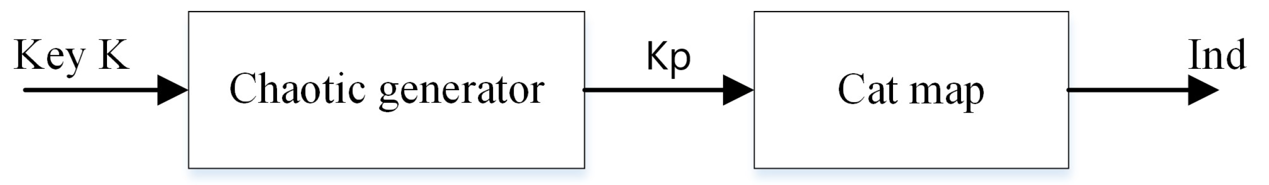
Figure 1.
Proposed chaotic generator.
Figure 1.
Proposed chaotic generator.
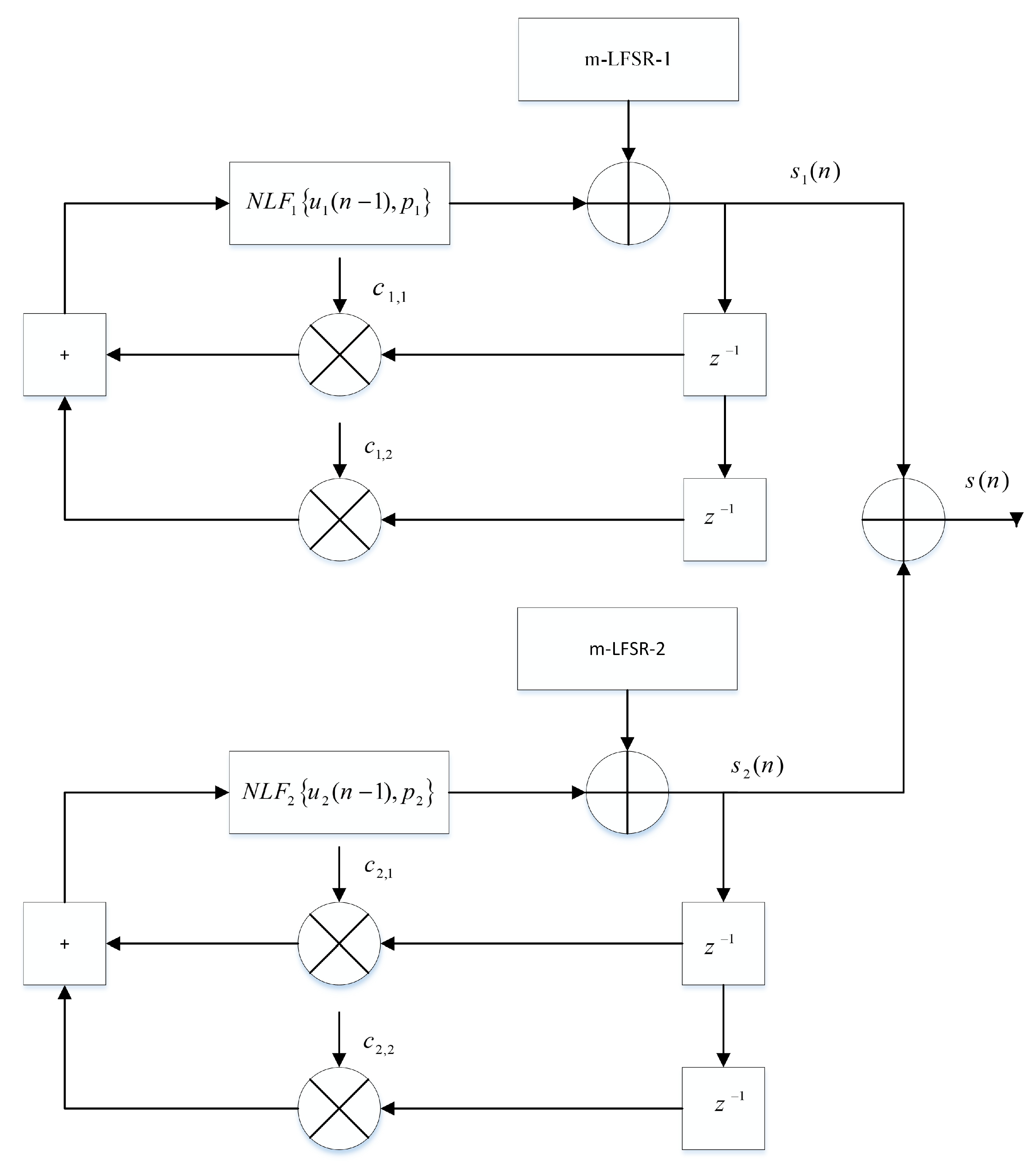
Figure 2.
Chaotic generator.
Figure 2.
Chaotic generator.
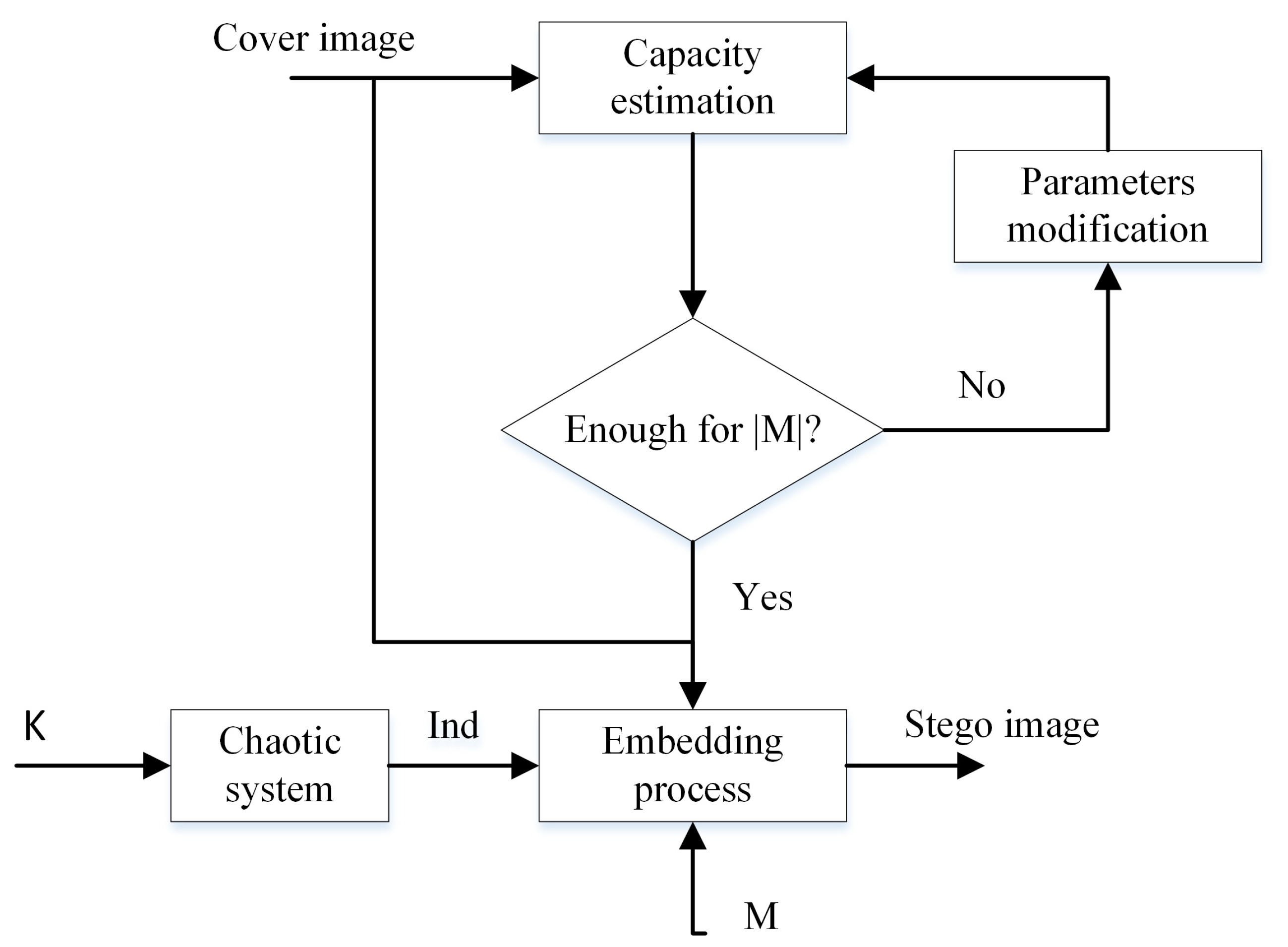
Figure 3.
EEALSBMR insertion procedure.
Figure 3.
EEALSBMR insertion procedure.
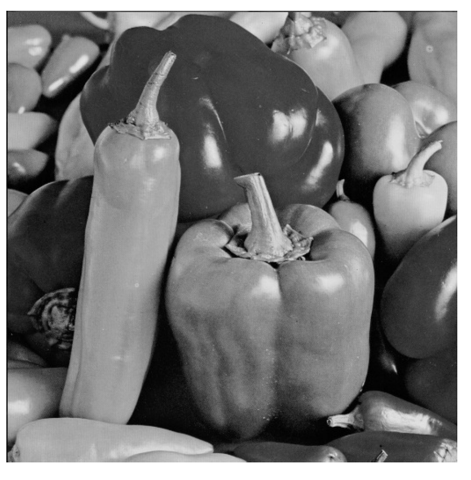
Figure 4.
“Peppers” as cover image.
Figure 4.
“Peppers” as cover image.
Figure 5.
“Bike” is as embedded message.
Figure 5.
“Bike” is as embedded message.
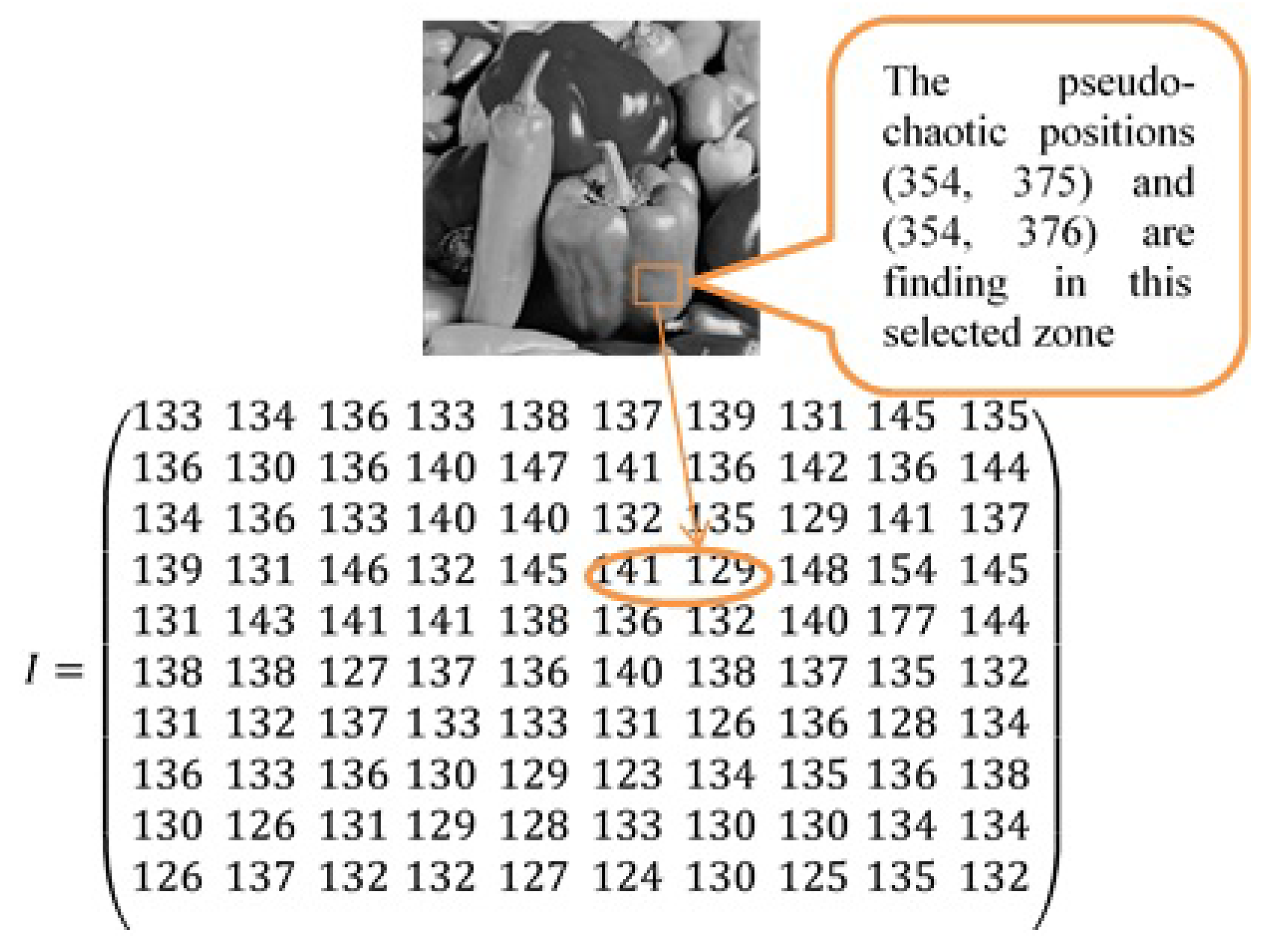
Figure 6.
Pseudo-chaotic block selection and its corresponding gray value.
Figure 6.
Pseudo-chaotic block selection and its corresponding gray value.
Figure 7.
Diagram of the enhanced steganographic-based DCT transform.
Figure 7.
Diagram of the enhanced steganographic-based DCT transform.
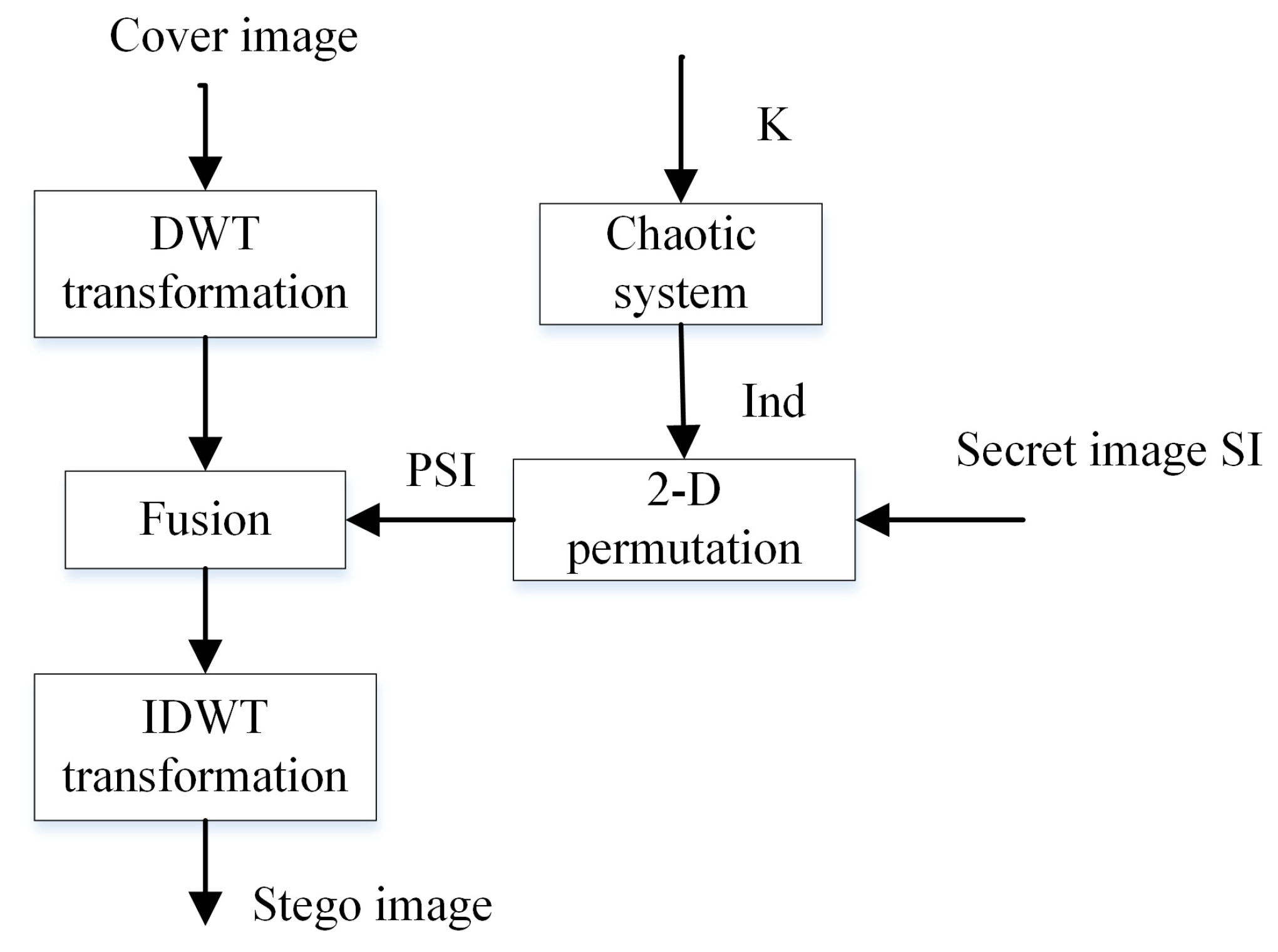
Figure 8.
Diagram of the EDWT algorithm.
Figure 8.
Diagram of the EDWT algorithm.
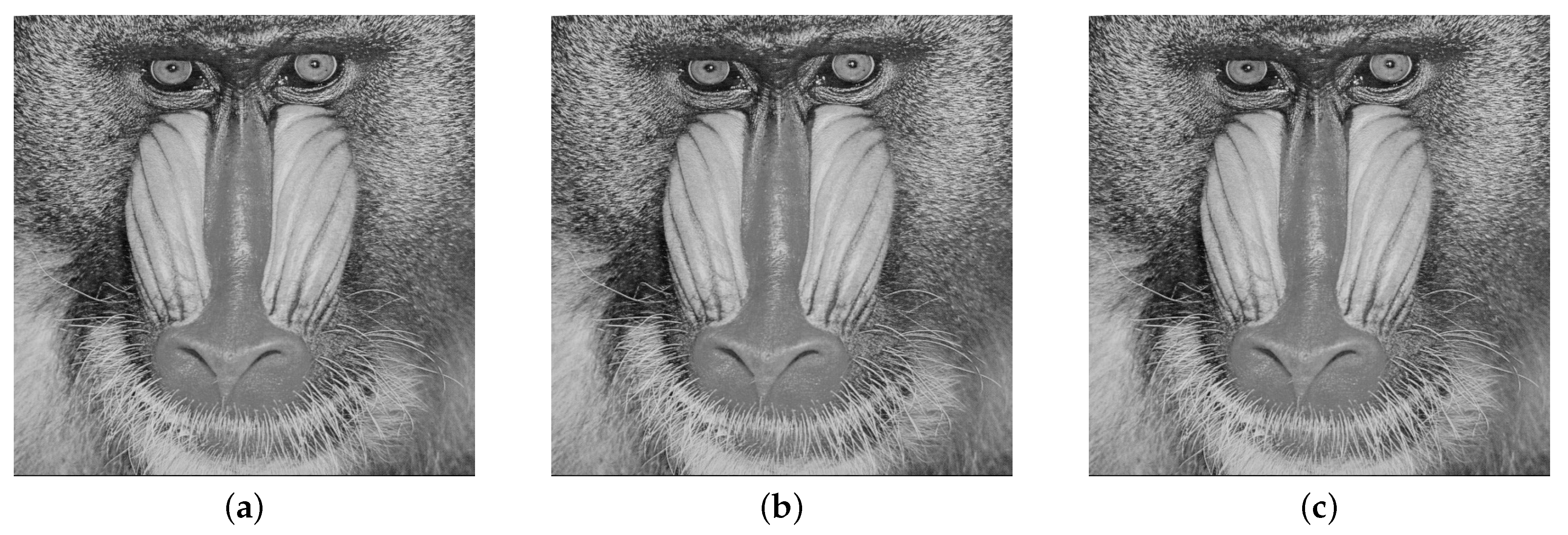
Figure 9.
(a) Cover image, (b) Stego image with embedding rate of 5%, (c) Stego image with embedding rate of 40%.
Figure 9.
(a) Cover image, (b) Stego image with embedding rate of 5%, (c) Stego image with embedding rate of 40%.
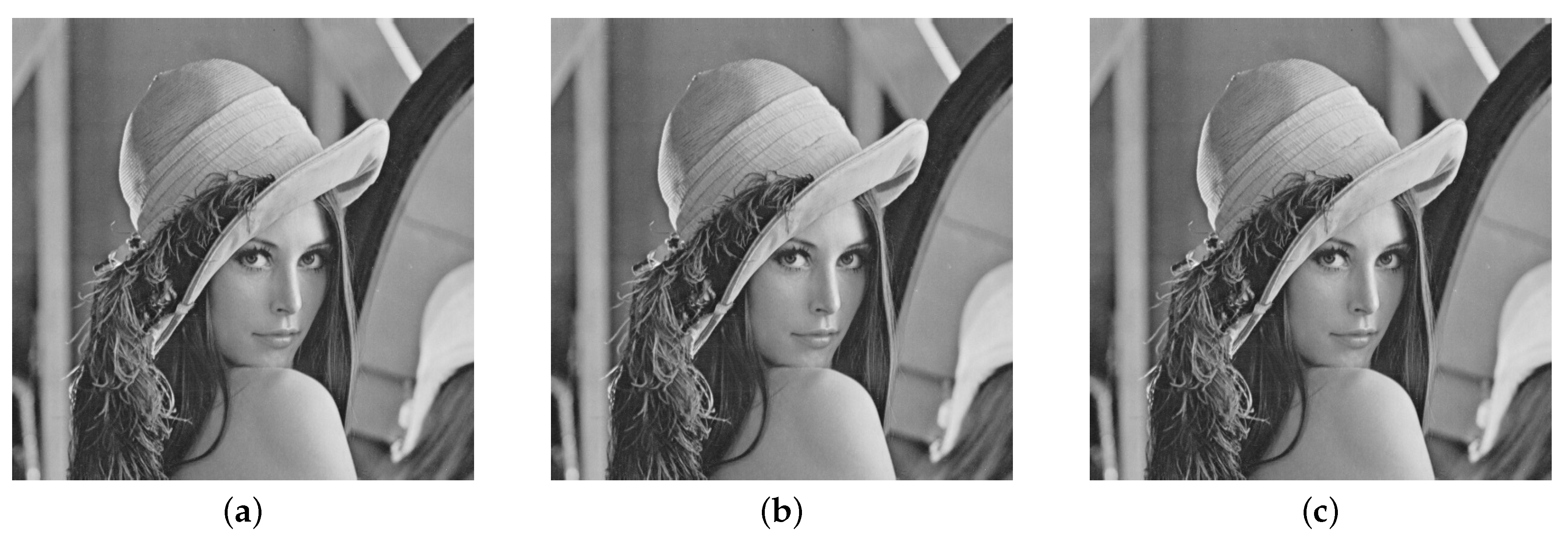
Figure 10.
(a) Cover image, (b) Stego image with embedding rate of 5%, (c) Stego image with embedding rate of 40%.
Figure 10.
(a) Cover image, (b) Stego image with embedding rate of 5%, (c) Stego image with embedding rate of 40%.
Figure 11.
(a) Cover image, (b) Stego image with embedding rate of 5%, (c) Stego image with embedding rate of 40%.
Figure 11.
(a) Cover image, (b) Stego image with embedding rate of 5%, (c) Stego image with embedding rate of 40%.
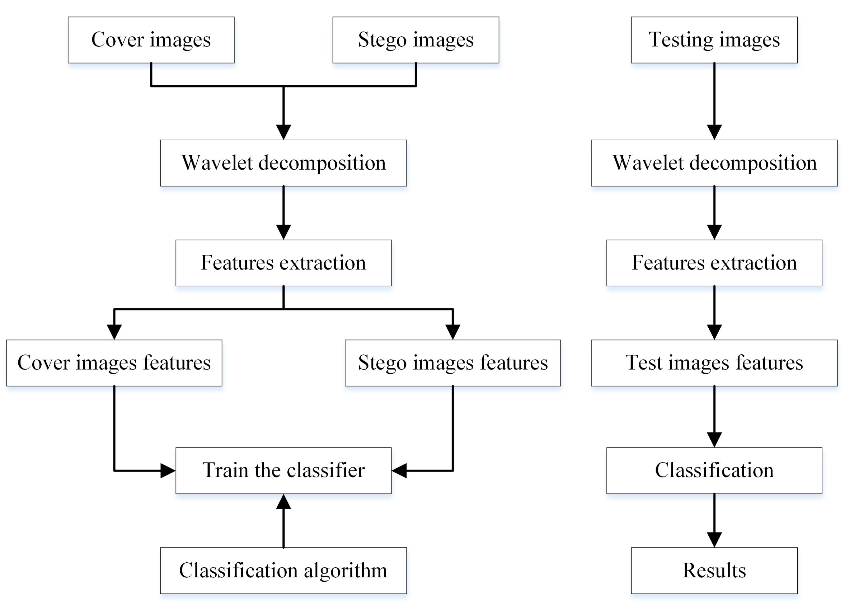
Figure 12.
Flowchart of the blind steganalysis process.
Figure 12.
Flowchart of the blind steganalysis process.
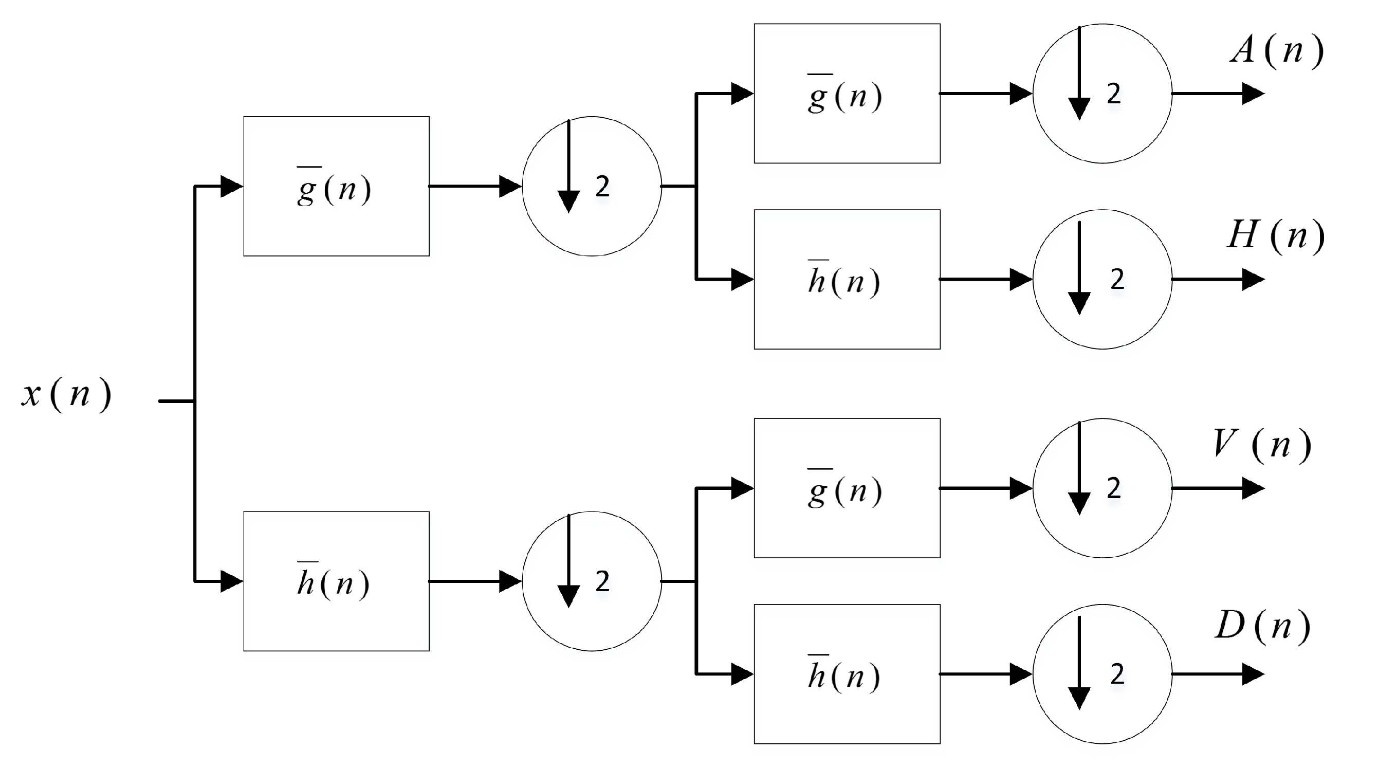
Figure 13.
Multi-resolution wavelet decomposition.
Figure 13.
Multi-resolution wavelet decomposition.
Figure 14.
Block diagram for the prediction of coefficient .
Figure 14.
Block diagram for the prediction of coefficient .
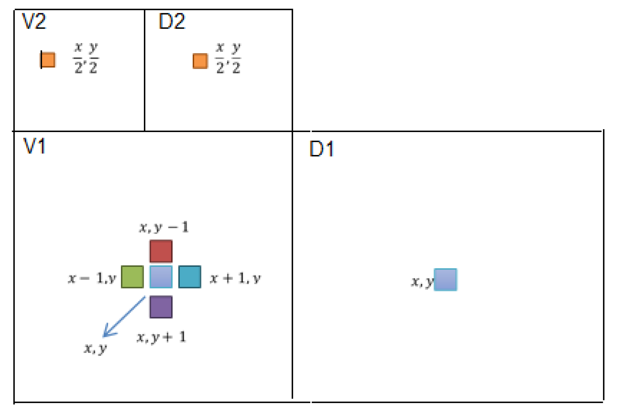
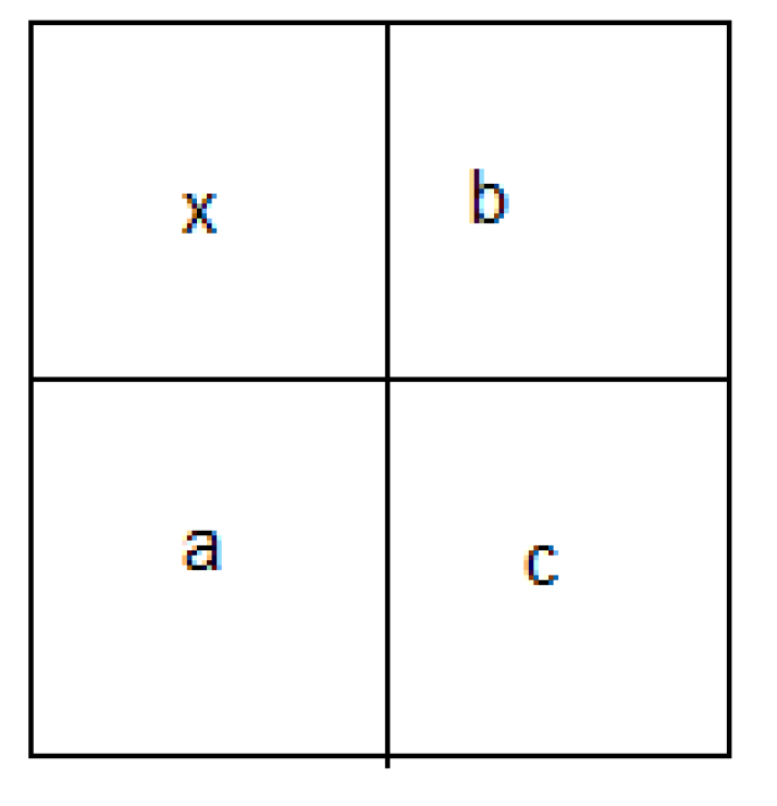
Figure 15.
Prediction context of a pixel x.
Figure 15.
Prediction context of a pixel x.
Table 1.
, , and values for the EEALSBMR method.
Table 1.
, , and values for the EEALSBMR method.
| Embedding Rate | Cover Image | | | |
|---|
| 5% | Baboon | 68.3810 | 0.9999 | 0.9999 |
| Lena | 68.1847 | 0.9999 | 0.9999 |
| Peppers | 67.7160 | 0.9999 | 0.9999 |
| 10% | Baboon | 65.5986 | 0.9999 | 0.9999 |
| Lena | 65.2821 | 0.9999 | 0.9999 |
| Peppers | 64.7763 | 0.9999 | 0.9999 |
| 20% | Baboon | 62.3551 | 0.9999 | 0.9999 |
| Lena | 62.3559 | 0.9999 | 0.9996 |
| Peppers | 61.7066 | 0.9999 | 0.9995 |
| 30% | Baboon | 60.6902 | 0.9998 | 0.9999 |
| Lena | 60.5630 | 0.9998 | 0.9990 |
| Peppers | 59.9585 | 0.9998 | 0.9992 |
| 40% | Baboon | 59.4245 | 0.9997 | 0.9999 |
| Lena | 59.2608 | 0.9997 | 0.9985 |
| Peppers | 58.6662 | 0.9997 | 0.9988 |
Table 2.
, , and values for the EDCT method.
Table 2.
, , and values for the EDCT method.
| Embedding Rate | Cover Image | | | |
|---|
| 5% | Baboon | 71.2372 | 0.9999 | 0.9999 |
| Lena | 71.1769 | 0.9999 | 0.9999 |
| Peppers | 70.4866 | 0.9999 | 0.9999 |
| 10% | Baboon | 64.8846 | 0.9999 | 0.9999 |
| Lena | 64.9487 | 0.9999 | 0.9998 |
| Peppers | 64.1426 | 0.9999 | 0.9998 |
| 20% | Baboon | 59.6895 | 0.9997 | 0.9999 |
| Lena | 59.6225 | 0.9997 | 0.9992 |
| Peppers | 58.9535 | 0.9997 | 0.9993 |
| 30% | Baboon | 57.4212 | 0.9995 | 0.9998 |
| Lena | 57.3421 | 0.9995 | 0.9989 |
| Peppers | 56.7406 | 0.9995 | 0.9988 |
| 40% | Baboon | 56.3421 | 0.9994 | 0.9997 |
| Lena | 56.2265 | 0.79994 | 0.9987 |
| Peppers | 55.4876 | 0.9994 | 0.9985 |
Table 3.
, , and values for EDWT method.
Table 3.
, , and values for EDWT method.
| Embedding Rate | Cover Image | | | |
|---|
| 5% | Baboon | 59.1876 | 0.9999 | 0.9999 |
| Lena | 58.7673 | 0.9997 | 0.9999 |
| Peppers | 58.1699 | 0.9997 | 0.9999 |
| 10% | Baboon | 56.2224 | 0.9997 | 0.9999 |
| Lena | 55.8085 | 0.9994 | 0.9999 |
| Peppers | 55.2086 | 0.9993 | 0.9999 |
| 20% | Baboon | 53.3463 | 0.9988 | 0.9999 |
| Lena | 52.8205 | 0.9988 | 0.9999 |
| Peppers | 52.2269 | 0.9987 | 0.9999 |
| 30% | Baboon | 52.0465 | 0.9984 | 0.9999 |
| Lena | 51.6471 | 0.9984 | 0.9999 |
| Peppers | 51.0509 | 0.9983 | 0.9999 |
| 40% | Baboon | 51.3450 | 0.9982 | 0.9999 |
| Lena | 50.9536 | 0.9981 | 0.9999 |
| Peppers | 50.3417 | 0.9980 | 0.9999 |
Table 4.
E, R, and for the EEALSBMR method.
Table 4.
E, R, and for the EEALSBMR method.
| Embedding Rate | Cover Image | E | R | |
|---|
| 5% | Baboon | 7.3586 | 0.0802 | 0.3805 |
| Lena | 7.4455 | 0.0693 | 0.3261 |
| Peppers | 7.5715 | 0.0536 | 0.2975 |
| 10% | Baboon | 7.3586 | 0.0802 | 0.3805 |
| Lena | 7.4456 | 0.0693 | 0.3261 |
| Peppers | 7.5715 | 0.0535 | 0.2976 |
| 20% | Baboon | 7.3585 | 0.0802 | 0.3805 |
| Lena | 7.4457 | 0.0693 | 0.3261 |
| Peppers | 7.5717 | 0.0535 | 0.2977 |
| 30% | Baboon | 7.3584 | 0.0802 | 0.3805 |
| Lena | 7.4457 | 0.0693 | 0.3261 |
| Peppers | 7.5718 | 0.0535 | 0.2975 |
| 40% | Baboon | 7.3578 | 0.0803 | 0.3806 |
| Lena | 7.4454 | 0,0693 | 0.3260 |
| Peppers | 7.5722 | 0.0535 | 0.2973 |
Table 5.
E, R, and values for the EDCT method.
Table 5.
E, R, and values for the EDCT method.
| Embedding Rate | Cover Image | E | R | |
|---|
| 5% | Baboon | 7.3585 | 0.0802 | 0.3804 |
| Lena | 7.4456 | 0.0693 | 0.3261 |
| Peppers | 7.5716 | 0.0536 | 0.2976 |
| 10% | Baboon | 7.3585 | 0.0802 | 0.3805 |
| Lena | 7.4456 | 0.0693 | 0.3262 |
| Peppers | 7.5717 | 0.0535 | 0.2976 |
| 20% | Baboon | 7.3585 | 0.0802 | 0.3804 |
| Lena | 7.4457 | 0.0693 | 0.3263 |
| Peppers | 7.5725 | 0.0534 | 0.2973 |
| 30% | Baboon | 7.3584 | 0.0802 | 0.3802 |
| Lena | 7.4459 | 0.0693 | 0.3261 |
| Peppers | 7.5730 | 0.0534 | 0.2969 |
| 40% | Baboon | 7.3578 | 0.0803 | 0.3806 |
| Lena | 7.4462 | 0,0692 | 0.3257 |
| Peppers | 7.5734 | 0.0533 | 0.2973 |
Table 6.
E, R, and values for EDWT method.
Table 6.
E, R, and values for EDWT method.
| Embedding Rate | Cover Image | E | R | |
|---|
| 5% | Baboon | 7.3581 | 0.0802 | 0.3805 |
| Lena | 7.4455 | 0.0693 | 0.3261 |
| Peppers | 7.5715 | 0.0536 | 0.2975 |
| 10% | Baboon | 7.3580 | 0.0802 | 0.3806 |
| Lena | 7.4456 | 0.0693 | 0.3261 |
| Peppers | 7.5717 | 0.0535 | 0.2974 |
| 20% | Baboon | 7.3580 | 0.0802 | 0.3806 |
| Lena | 7.4456 | 0.0693 | 0.3261 |
| Peppers | 7.5718 | 0.0535 | 0.2975 |
| 30% | Baboon | 7.3580 | 0.0802 | 0.3805 |
| Lena | 7.4456 | 0.0693 | 0.3261 |
| Peppers | 7.5718 | 0.0535 | 0.2974 |
| 40% | Baboon | 7.3580 | 0.0803 | 0.3806 |
| Lena | 7.4457 | 0,0693 | 0.3261 |
| Peppers | 7.5721 | 0.0533 | 0.2973 |
Table 7.
E, R, and values for the cover images.
Table 7.
E, R, and values for the cover images.
| Cover Image | E | R | |
|---|
| Baboon | 7.3585 | 0.0802 | 0.3805 |
| Lena | 7.4455 | 0.0693 | 0.3261 |
| Peppers | 7.5715 | 0.0536 | 0.2976 |
Table 8.
Confusion matrix.
Table 8.
Confusion matrix.
| | | H0: Stego Image | H1: Cover Image | |
|---|
Test
outcome | Test
outcome
positive | True Positive
| False Positive
| Positive predictive
value (),
or Precision
|
| | Test
outcome
negative | False Negative
| True Negative
| Negative predictive
value ()
|
| | | True positive rate (),
or, Sensitivity (),
| True negative
rate (),
or Specificity(),
| Accuracy (),
|
Table 9.
FLD classification evaluation of EEALSBMR algorithm using Farid features.
Table 9.
FLD classification evaluation of EEALSBMR algorithm using Farid features.
| 5% | H0: Stego Images | H1: Cover Images | |
| H0 | 0.2744 | 0.2714 | = 0.5027 |
| H1 | 0.2256 | 0.2286 | = 0.5033 |
| | = 0.5487 | = 0.4572 | = 0.5030 |
| = 0.0060 |
| 10% | H0: Stego Images | H1: Cover Images | |
| H0 | 0.2690 | 0.2645 | = 0.5042 |
| H1 | 0.2310 | 0.2355 | = 0.5048 |
| | = 0.5380 | = 0.4710 | = 0.5045 |
| = 0.0090 |
| 20% | H0: Stego Images | H1: Cover Images | |
| H0 | 0.2745 | 0.2459 | = 0.5275 |
| H1 | 0.2255 | 0.2541 | = 0.5298 |
| | = 0.5490 | = 0.5082 | = 0.5286 |
| = 0.0572 |
Table 10.
FLD classification evaluation of EEALSBMR algorithm using Shi features.
Table 10.
FLD classification evaluation of EEALSBMR algorithm using Shi features.
| 5% | H0: Stego Images | H1: Cover Images | |
| H0 | 0.2612 | 0.2405 | = 0.5207 |
| H1 | 0.2387 | 0.2595 | = 0.5208 |
| | = 0.5225 | = 0.5190 | = 0.5208 |
| = 0.0415 |
| 10% | H0: Stego Images | H1: Cover Images | |
| H0 | 0.2504 | 0.2448 | = 0.5057 |
| H1 | 0.2496 | 0.2552 | = 0.5056 |
| | = 0.5008 | = 0.5105 | = 0.5056 |
| = 0.0112 |
| 20% | H0: Stego Images | H1: Cover Images | |
| H0 | 0.3191 | 0.1946 | = 0.6212 |
| H1 | 0.1809 | 0.3054 | = 0.6280 |
| | = 0.6382 | = 0.6108 | = 0.6245 |
| = 0.2490 |
Table 11.
FLD classification evaluation of EEALSBMR algorithm using Moulin features.
Table 11.
FLD classification evaluation of EEALSBMR algorithm using Moulin features.
| 5% | H0: Stego Images | H1: Cover Images | |
| H0 | 0.2489 | 0.2476 | = 0.5013 |
| H1 | 0.2511 | 0.2524 | = 0.5012 |
| | = 0.4977 | = 0.5048 | = 0.5012 |
| = 0.0025 |
| 10% | H0: Stego Images | H1: Cover Images | |
| H0 | 0.2559 | 0.2299 | = 0.5268 |
| H1 | 0.2441 | 0.2701 | = 0.5253 |
| | = 0.5117 | = 0.5403 | = 0.5260 |
| = 0.0520 |
| 20% | H0: Stego Images | H1: Cover Images | |
| H0 | 0.2990 | 0.1985 | = 0.6010 |
| H1 | 0.2010 | 0.3015 | = 0.6000 |
| | = 0.5980 | = 0.6030 | = 0.6005 |
| = 0.2010 |
Table 12.
SVM classification evaluation of EEALSBMR algorithm using Farid features.
Table 12.
SVM classification evaluation of EEALSBMR algorithm using Farid features.
| 5% | H0: Stego Images | H1: Cover Images | |
| H0 | 0.3438 | 0.3431 | = 0.5005 |
| H1 | 0.1562 | 0.1569 | = 0.5011 |
| | = 0.6876 | = 0.3137 | = 0.6870 |
| = 0.0013 |
| 10% | H0: Stego Images | H1: Cover Images | |
| H0 | 0.4006 | 0.3977 | = 0.5018 |
| H1 | 0.0994 | 0.1023 | = 0.5071 |
| | = 0.8011 | = 0.2046 | = 0.5029 |
| = 0.0057 |
| 20% | H0: Stego Images | H1: Cover Images | |
| H0 | 0.3251 | 0.3199 | = 0.5041 |
| H1 | 0.1749 | 0.1801 | = 0.5074 |
| | = 0.6503 | = 0.3602 | = 0.5052 |
| = 0.0105 |
Table 13.
SVM classification evaluation of EEALSBMR algorithm using Shi features.
Table 13.
SVM classification evaluation of EEALSBMR algorithm using Shi features.
| 5% | H0: Stego Images | H1: Cover Images | |
| H0 | 0.2220 | 0.2188 | = 0.5037 |
| H1 | 0.2780 | 0.2812 | = 0.5029 |
| | = 0.4440 | = 0.5625 | = 0.5032 |
| = 0.0065 |
| 10% | H0: Stego Images | H1: Cover Images | |
| H0 | 0.2189 | 0.2161 | = 0.5032 |
| H1 | 0.2811 | 0.2839 | = 0.5024 |
| | = 0.4377 | = 0.5678 | = 0.5028 |
| = 0.0055 |
| 20% | H0: Stego Images | H1: Cover Images | |
| H0 | 0.2282 | 0.1999 | = 0.5330 |
| H1 | 0.2718 | 0.3001 | = 0.5247 |
| | = 0.4564 | = 0.6002 | = 0.5283 |
| = 0.0566 |
Table 14.
SVM classification evaluation of EEALSBMR algorithm using Moulin features.
Table 14.
SVM classification evaluation of EEALSBMR algorithm using Moulin features.
| 5% | H0: Stego Images | H1: Cover Images | |
| H0 | 0.2275 | 0.2264 | = 0.5013 |
| H1 | 0.2725 | 0.2736 | = 0.5010 |
| | = 0.4550 | = 0.5472 | = 0.5011 |
| = 0.0023 |
| 10% | H0: Stego Images | H1: Cover Images | |
| H0 | 0.2412 | 0.2380 | = 0.5034 |
| H1 | 0.2588 | 0.2620 | = 0.5031 |
| | = 0.4825 | = 0.5240 | = 0.5032 |
| = 0.0065 |
| 20% | H0: Stego Images | H1: Cover Images | |
| H0 | 0.2922 | 0.2684 | = 0.5212 |
| H1 | 0.2078 | 0.2316 | = 0.5271 |
| | = 0.5844 | = 0.4632 | = 0.5238 |
| = 0.0476 |
Table 15.
FLD classification evaluation of EDCT algorithm using Farid features.
Table 15.
FLD classification evaluation of EDCT algorithm using Farid features.
| 5% | H0: Stego Images | H1: Cover Images | |
| H0 | 0.2524 | 0.2454 | = 0.5070 |
| H1 | 0.2476 | 0.2546 | = 0.5069 |
| | = 0.5048 | = 0.5091 | = 0.5070 |
| = 0.0139 |
| 10% | H0: Stego Images | H1: Cover Images | |
| H0 | 0.2617 | 0.2238 | = 0.5390 |
| H1 | 0.2383 | 0.2762 | = 0.5368 |
| | = 0.5234 | = 0.5524 | = 0.5379 |
| = 0.0758 |
| 20% | H0: Stego Images | H1: Cover Images | |
| H0 | 0.3104 | 0.1719 | = 0.6436 |
| H1 | 0.1896 | 0.3281 | = 0.6337 |
| | = 0.6208 | = 0.6562 | = 0.6385 |
| = 0.2770 |
Table 16.
FLD classification evaluation of EDCT algorithm using Shi features.
Table 16.
FLD classification evaluation of EDCT algorithm using Shi features.
| 5% | H0: Stego Images | H1: Cover Images | |
| H0 | 0.2548 | 0.2343 | = 0.5209 |
| H1 | 0.2452 | 0.2657 | = 0.5200 |
| | = 0.5095 | = 0.5314 | = 0.5205 |
| = 0.0410 |
| 10% | H0: Stego Images | H1: Cover Images | |
| H0 | 0.3242 | 0.1893 | = 0.6313 |
| H1 | 0.1758 | 0.3107 | = 0.6386 |
| | = 0.6484 | = 0.6213 | = 0.6349 |
| = 0.2697 |
| 20% | H0: Stego Images | H1: Cover Images | |
| H0 | 0.4409 | 0.0635 | = 0.8741 |
| H1 | 0.0591 | 0.4365 | = 0.8807 |
| | = 0.8817 | = 0.8730 | = 0.8773 |
| = 0.7547 |
Table 17.
FLD classification evaluation of EDCT algorithm using Moulin features.
Table 17.
FLD classification evaluation of EDCT algorithm using Moulin features.
| 5% | H0: Stego Images | H1: Cover Images | |
| H0 | 0.2611 | 0.2499 | = 0.5110 |
| H1 | 0.2389 | 0.2501 | = 0.5115 |
| | = 0.5223 | = 0.5002 | = 0.5112 |
| = 0.0225 |
| 10% | H0: Stego Images | H1: Cover Images | |
| H0 | 0.2780 | 0.2136 | = 0.5655 |
| H1 | 0.2220 | 0.2864 | = 0.5633 |
| | = 0.5560 | = 0.5728 | = 0.5644 |
| = 0.1288 |
| 20% | H0: Stego Images | H1: Cover Images | |
| H0 | 0.3739 | 0.1243 | = 0.7505 |
| H1 | 0.1261 | 0.3757 | = 0.7487 |
| | = 0.7478 | = 0.7514 | = 0.7496 |
| = 0.4992 |
Table 18.
SVM classification evaluation of EDCT algorithm using Farid features.
Table 18.
SVM classification evaluation of EDCT algorithm using Farid features.
| 5% | H0: Stego Images | H1: Cover Images | |
| H0 | 0.0653 | 0.0591 | = 0.5249 |
| H1 | 0.4347 | 0.4409 | = 0.5035 |
| | = 0.1307 | = 0.8817 | = 0.5062 |
| = 0.0124 |
| 10% | H0: Stego Images | H1: Cover Images | |
| H0 | 0.0848 | 0.0644 | = 0.5683 |
| H1 | 0.4152 | 0.4356 | = 0.5120 |
| | = 0.1695 | = 0.8712 | = 0.5204 |
| = 0.0408 |
| 20% | H0: Stego Images | H1: Cover Images | |
| H0 | 0.1734 | 0.0843 | = 0.6729 |
| H1 | 0.3266 | 0.4157 | = 0.5600 |
| | = 0.3469 | = 0.8314 | = 0.5891 |
| = 0.1783 |
Table 19.
SVM classification evaluation of EDCT algorithm using Shi features.
Table 19.
SVM classification evaluation of EDCT algorithm using Shi features.
| 5% | H0: Stego Images | H1: Cover Images | |
| H0 | 0.3156 | 0.3138 | = 0.5014 |
| H1 | 0.1844 | 0.1862 | = 0.5024 |
| | = 0.6312 | = 0.3724 | = 0.5018 |
| = 0.0036 |
| 10% | H0: Stego Images | H1: Cover Images | |
| H0 | 0.3572 | 0.3266 | = 0.5224 |
| H1 | 0.1428 | 0.1734 | = 0.5485 |
| | = 0.7145 | = 0.3469 | = 0.5307 |
| = 0.0613 |
| 20% | H0: Stego Images | H1: Cover Images | |
| H0 | 0.4217 | 0.2220 | = 0.6551 |
| H1 | 0.0783 | 0.2780 | = 0.7803 |
| | = 0.8434 | = 0.5560 | = 0.6997 |
| = 0.3994 |
Table 20.
SVM classification evaluation of EDCT algorithm using Moulin features.
Table 20.
SVM classification evaluation of EDCT algorithm using Moulin features.
| 5% | H0: Stego Images | H1: Cover Images | |
| H0 | 0.3053 | 0.3020 | = 0.5027 |
| H1 | 0.1947 | 0.1980 | = 0.5042 |
| | = 0.6107 | = 0.3960 | = 0.5033 |
| = 0.0067 |
| 10% | H0: Stego Images | H1: Cover Images | |
| H0 | 0.3021 | 0.2924 | = 0.5082 |
| H1 | 0.1979 | 0.2076 | = 0.5120 |
| | = 0.6042 | = 0.4152 | = 0.5097 |
| = 0.0194 |
| 20% | H0: Stego Images | H1: Cover Images | |
| H0 | 0.3264 | 0.2427 | = 0.5736 |
| H1 | 0.1736 | 0.2573 | = 0.5971 |
| | = 0.6528 | = 0.5147 | = 0.5837 |
| = 0.1674 |
Table 21.
FLD classification evaluation of EDWT algorithm using Farid features.
Table 21.
FLD classification evaluation of EDWT algorithm using Farid features.
| 5% | H0: Stego Images | H1: Cover Images | |
| H0 | 0.4786 | 0.0150 | = 0.9695 |
| H1 | 0.0214 | 0.4850 | = 0.9577 |
| | = 0.9571 | = 0.9699 | = 0.9635 |
| = 0.9270 |
| 10% | H0: Stego Images | H1: Cover Images | |
| H0 | 0.4941 | 0.0056 | = 0.9888 |
| H1 | 0.0059 | 0.4944 | = 0.9882 |
| | = 0.9882 | = 0.9888 | = 0.9885 |
| = 0.9770 |
| 20% | H0: Stego Images | H1: Cover Images | |
| H0 | 0.4993 | 0.0005 | = 0.9990 |
| H1 | 0.0007 | 0.4995 | = 0.9987 |
| | = 0.9987 | = 0.9990 | = 0.9989 |
| = 0.9977 |
Table 22.
FLD classification evaluation of EDWT algorithm using Shi features.
Table 22.
FLD classification evaluation of EDWT algorithm using Shi features.
| 5% | H0: Stego Images | H1: Cover Images | |
| H0 | 0.4048 | 0.0470 | = 0.8961 |
| H1 | 0.0952 | 0.4530 | = 0.8263 |
| | = 0.8095 | = 0.9061 | = 0.8578 |
| = 0.7156 |
| 10% | H0: Stego Images | H1: Cover Images | |
| H0 | 0.4536 | 0.0311 | = 0.9358 |
| H1 | 0.0464 | 0.4689 | = 0.9100 |
| | = 0.9072 | = 0.9377 | = 0.9225 |
| = 0.8450 |
| 20% | H0: Stego Images | H1: Cover Images | |
| H0 | 0.4753 | 0.0232 | = 0.9534 |
| H1 | 0.0247 | 0.4768 | = 0.9508 |
| | = 0.9507 | = 0.9535 | = 0.9521 |
| = 0.9042 |
Table 23.
FLD classification evaluation of EDWT algorithm using Moulin features.
Table 23.
FLD classification evaluation of EDWT algorithm using Moulin features.
| 5% | H0: Stego Images | H1: Cover Images | |
| H0 | 0.3946 | 0.0650 | = 0.8587 |
| H1 | 0.1054 | 0.4350 | = 0.8049 |
| | = 0.7891 | = 0.8701 | = 0.8296 |
| = 0.6592 |
| 10% | H0: Stego Images | H1: Cover Images | |
| H0 | 0.4394 | 0.0387 | = 0.9191 |
| H1 | 0.0606 | 0.4613 | = 0.8839 |
| | = 0.8789 | = 0.9227 | = 0.9008 |
| = 0.8015 |
| 20% | H0: Stego Images | H1: Cover Images | |
| H0 | 0.4603 | 0.0321 | = 0.9348 |
| H1 | 0.0397 | 0.4679 | = 0.9218 |
| | = 0.9206 | = 0.9358 | = 0.9282 |
| = 0.8564 |
Table 24.
SVM classification evaluation of EDWT algorithm using Farid features.
Table 24.
SVM classification evaluation of EDWT algorithm using Farid features.
| 5% | H0: Stego Images | H1: Cover Images | |
| H0 | 0.4770 | 0.0230 | = 0.9541 |
| H1 | 0.0230 | 0.4770 | = 0.9541 |
| | = 0.9541 | = 0.9541 | = 0.9541 |
| = 0.9082 |
| 10% | H0: Stego Images | H1: Cover Images | |
| H0 | 0.4893 | 0.0058 | = 0.9883 |
| H1 | 0.0107 | 0.4942 | = 0.9789 |
| | = 0.9787 | = 0.9884 | = 0.9835 |
| = 0.9670 |
| 20% | H0: Stego Images | H1: Cover Images | |
| H0 | 0.4984 | 0.0084 | = 0.9835 |
| H1 | 0.0016 | 0.4916 | = 0.9967 |
| | = 0.9968 | = 0.9832 | = 0.9900 |
| = 0.9800 |
Table 25.
SVM classification evaluation of EDWT algorithm using Shi features.
Table 25.
SVM classification evaluation of EDWT algorithm using Shi features.
| 5% | H0: Stego Images | H1: Cover Images | |
| H0 | 0.3366 | 0.1658 | = 0.6700 |
| H1 | 0.1634 | 0.3342 | = 0.6716 |
| | = 0.6731 | = 0.6684 | = 0.6708 |
| = 0.3415 |
| 10% | H0: Stego Images | H1: Cover Images | |
| H0 | 0.4107 | 0.1371 | = 0.7497 |
| H1 | 0.0893 | 0.3629 | = 0.8024 |
| | = 0.8213 | = 0.7257 | = 0.7735 |
| = 0.5470 |
| 20% | H0: Stego Images | H1: Cover Images | |
| H0 | 0.4605 | 0.1175 | = 0.7967 |
| H1 | 0.0395 | 0.3825 | = 0.9063 |
| | = 0.9210 | = 0.7650 | = 0.8430 |
| = 0.6859 |
Table 26.
SVM classification evaluation of EDWT algorithm using Moulin features.
Table 26.
SVM classification evaluation of EDWT algorithm using Moulin features.
| 5% | H0: Stego Images | H1: Cover Images | |
| H0 | 0.3707 | 0.1108 | = 0.7699 |
| H1 | 0.1293 | 0.3892 | = 0.7506 |
| | = 0.7413 | = 0.7785 | = 0.7599 |
| = 0.5198 |
| 10% | H0: Stego Images | H1: Cover Images | |
| H0 | 0.4332 | 0.0725 | = 0.8567 |
| H1 | 0.0668 | 0.4275 | = 0.8649 |
| | = 0.8665 | = 0.8550 | = 0.8608 |
| = 0.7215 |
| 20% | H0: Stego Images | H1: Cover Images | |
| H0 | 0.4672 | 0.0724 | = 0.8659 |
| H1 | 0.0668 | 0.4276 | = 0.9288 |
| | = 0.9345 | = 0.8552 | = 0.8949 |
| = 0.7897 |

 ,
, 


