Gaussian Process Based Expected Information Gain Computation for Bayesian Optimal Design


1
School of Information Science and Technology, ShanghaiTech University, Shanghai 201210, China
2
Shanghai Institute of Microsystem and Information Technology, Chinese Academy of Sciences, Shanghai 200050, China
3
University of Chinese Academy of Sciences, Beijing 100049, China
*
Author to whom correspondence should be addressed.
Entropy 2020, 22(2), 258; https://0-doi-org.brum.beds.ac.uk/10.3390/e22020258
Submission received: 6 January 2020
/
Revised: 15 February 2020
/
Accepted: 19 February 2020
/
Published: 24 February 2020
(This article belongs to the Section Multidisciplinary Applications)
Abstract
:Optimal experimental design (OED) is of great significance in efficient Bayesian inversion. A popular choice of OED methods is based on maximizing the expected information gain (EIG), where expensive likelihood functions are typically involved. To reduce the computational cost, in this work, a novel double-loop Bayesian Monte Carlo (DLBMC) method is developed to efficiently compute the EIG, and a Bayesian optimization (BO) strategy is proposed to obtain its maximizer only using a small number of samples. For Bayesian Monte Carlo posed on uniform and normal distributions, our analysis provides explicit expressions for the mean estimates and the bounds of their variances. The accuracy and the efficiency of our DLBMC and BO based optimal design are validated and demonstrated with numerical experiments.
1. Introduction
As acquiring data in experiments is generally computationally demanding and time-consuming, maximizing the informativeness of experimental data is of crucial importance. For example, in the area of climate science, a complex system with various stochastic inputs is integrated to represent the real climate situation. Usually, the locations and the time of putting sensors to collect climate observations are optional. With limited resources, careful selections of sensor placements are required (see Reference [1] for a detailed discussion). Many works focus on finding experimental data carrying more information, and this topic is usually referred to as optimal experimental design (OED) [2]. In this paper, we consider the OED problem in the context of the Bayesian inverse problem. Given a forward problem, the inverse problem is to infer parameters inherent of the forward model through a set of design points and the corresponding responses. In the Bayesian setting, the parameters of interest are viewed as random variables, and hence the posterior distribution of the parameters can be obtained via the Bayes’ rules [3,4,5,6]. In linear cases, the OED problem includes various criteria such as the D-optimal design criterion and the A-optimal design criterion. The D-optimal design criterion seeks to maximize the determinant of the information matrix of the design, whereas the A-optimal design criterion considers minimizing the trace of the inverse of the information matrix which results in minimizing the average variance [7,8,9].
We focus on the decision theoretic approach that considers maximizing the expectation of Kullback-Leibler (KL) divergence from the posterior distribution to the prior distribution [10]. This decision theoretic approach is a nonlinear generalization of the Bayesian D-optimal criterion [11]. The objective function we want to maximize, the expectation of KL divergence, is also referred to as the expected information gain (EIG) over parameters. Computing EIG is usually a challenging problem, since it does not have an analytical form for nonlinear problems in general. In the literature, the following attempts have been made for this problem. Efficient surrogates for the forward models are introduced to make the problem tractable [1,12,13,14,15]. Recently, as the rise of novel computational methods, new approaches are actively developed to evaluate the EIG, including the quasi-Monte Carlo method [16] and the layered importance sampling [17] in the context of the focused optimal design. As the goal of this kind of optimal design is to find the maximizer of EIG, it is crucial to apply efficient optimization strategies. In Reference [12], a curve fitting surrogate of Monte Carlo experiments is proposed to result in an efficient optimization scheme. For the Bayesian optimal design problem focusing on the risk from an optimal terminal decision, the Bayesian optimization (BO) approach is proposed to find the minimizer of the risk [9]. We note that, while BO is proposed for the Bayesian optimal design problem for minimizing the risk in Reference [9], BO is considered for maximizing the EIG in this work. In addition, efficient approximate coordinate exchange strategies are proposed for Bayesian design in Reference [18]. For intractable likelihood models, Gaussian process (GP) models are built to emulate the likelihood function in Reference [19]. Gradient-based optimization methods are proposed to compute the maximizer of EIG in References [13,14]. Review of modern computational methods for decision theoretic optimal experimental design is provided in Reference [20].
The main purpose of this work is to propose an efficient Gaussian process (GP) based Bayesian optimal design strategy, where Bayesian Monte Carlo (BMC) and Bayesian optimization (BO) which are both based on GP are used [21,22,23]. As the Monte Carlo simulation for EIG involves an inner layer simulation and an outer layer simulation (see Reference [14]), we develop a novel efficient double-loop Bayesian Monte Carlo (DLBMC) method, which employs BMC [24,25,26] for both layers. However, the EIG is generally computationally expensive and its gradient information is typically not given explicitly. We propose a BO method [27,28,29] to compute the maximizer of EIG, where the gradient information of EIG is not required. To summarize, the contributions of this work are three-fold: first we develop a novel DLBMC to efficiently compute EIG; second we analyze the BMC for the normal and the uniform distributions; third we propose BO to obtain the maximizer of EIG.
This paper is organized as follows. In Section 2, we review the Bayesian optimal experimental design problem and formulate the expected information gain (EIG) criterion. In Section 3, we derive a double-loop Bayesian Monte Carlo estimator for the EIG and propose a Bayesian optimization approach to obtain the maximizer of the approximated EIG. Detailed analysis of BMC for the normal and the uniform distributions are conducted in this section. In Section 4, we demonstrate the efficiency of our GP based Bayesian optimal design with three test problems. Section 5 concludes the paper and provides discussions of the advantages and disadvantages of our algorithm.
2. Formulation of Experimental Design
In this section, we review the setting of the Bayesian optimal design problem following the presentation in [14]. In the Bayesian setting, the unknown parameters are viewed as random variables. Let be a probability space, where is a sample space, is a -field, and is the probability measure on Let denote the parameters of interest, where is the dimension of the unknown parameters. Assume that is associated with a prior measure on satisfying for . Throughout this paper, we assume that all the random variables have densities with respect to the Lebesgue measure. Let denotes the design variable, where is the number of design variables and denotes the design space. Let denote the response associated with where is the dimension of response. The inference of can be obtained based on the prior distribution and observations via Bayes’ rule,
The likelihood function is often determined by a deterministic forward model and a statistical model for measurement of model noises. Here we model the relation of the design variable and the observation by a deterministic model and additive Gaussian noises ,
where is the forward model. In many practical problems, the forward model is computationally expensive, and its explicit form is not given. So we can just view it as a black box whose internal structure is unknown, whereas we can generate noisy responses given fixed design variables and parameters.
Following the decision theoretic approach [10], we set the utility function as the KL divergence from the posterior distribution to the prior distribution,
This term is actually independent of . Noting that is a function of both and , therefore we further take expectation of u over to define the expected information gain (EIG):
Then the optimal experimental design is to find a design point which maximizes the expected utility, that is,
A double-loop Monte Carlo (DLMC) estimator of EIG is proposed in [30]. Rewrite as
and note that , since the specification of does not provide further information about inference of Then, the DLMC method approximates as
where are drawn from the prior , and are drawn from the conditional distribution (i.e., the likelihood), and hence can be estimated via the importance sampling technique,
Combining (6) and (5) yields a biased estimator of . However, if we sample for every (), the complexity of this method is . To reduce the computational cost, a sample reuse technique is employed in [14]. That is, for every , we drawn a fresh batch from the prior and use this set for both the outer Monte Carlo and the inner Monte Carlo (i.e., ). Consequently, the complexity is reduced to .
3. GP Based Framework for Bayesian Optimal Design
Our main framework for Bayesian optimal design is based on two powerful tools according to Gaussian processes: the Bayesian Monte Carlo (BMC) method and the Bayesian optimization (BO) method. In this section, we first review BMC and conduct the analysis of BMC for the normal and the uniform distributions, and then present our novel double loop Bayesian Monte Carlo (DLBMC) for EIG. After that, we propose BO to find the maximizer of the approximated EIG. Finally, we review the classical Markov chain Monte Carlo (MCMC) method for Bayesian parameter inference.
3.1. Bayesian Monte Carlo
Consider the integral problem where is the density of x, is the integrand, and is the support of x, that is, the integration domain. The idea of BMC is to formulate an integral problem into a Bayesian inference problem by placing a prior over the integrand f and to obtain the posterior distribution of f conditioning on the data collected. A natural way of putting a prior over function is through a Gaussian process, which is completely characterized by its mean function and kernel function , that is, A commonly used choice for the kernel function is the Gaussian kernel (or known as squared exponential kernel), , where both and l are hyperparameters of the kernel function. The choice of hyperparameters affects the result to a large extent. Therefore the hyperparameters need to be determined carefully. Having collected noisy observations , where with Gaussian noises a Gaussian process provides a posterior distribution for an arbitrary new point , with mean function and variance function given by
where , , and In some special cases (For example, when x is distributed with Gaussian and the kernel is a Gaussian kernel [25]), GP allows us to estimate the integration in a closed form, of which the posterior mean is given by,
where , and the posterior variance is given by
Note that in the above analytical expression of posterior mean and variance, when the hyperparameters and the kernel function are given, z and K are determined by and they are independent of the observations . Therefore, the computation procedure for the posterior mean and variance of the BMC estimator proceeds the following two steps: first, an input sample set is generated, and z and K are computed; second, the corresponding observation set is collected, and the posterior mean and variance are computed through (7) and (8) respectively. Next, when x is an uniform or Gaussian random vector, we provide detailed derivations for the posterior mean and variance of BMC estimators.
Theorem 1
(Bayesian Monte Carlo for the standard Gaussian distribution). Consider the integral , where x is the standard Gaussian random variable vector in . The prior mean function is assumed to be a zero function, and the kernel is assumed to be the Gaussian kernel with predetermined hyperparameters and l. Having collected noisy observations where and , the posterior mean and variance of BMC are given by
where , , and the components of z are
for
Proof.
The components of z can be computed analytically, for
Moreover, the variance of BMC is
□
We note that Theorem 1 is presented in References [22,25], but we give the above detailed proof for completeness.
Theorem 2
(Bayesian Monte Carlo for the uniform distribution). Consider the integral , where x is a random vector uniformly distributed in the hypercube . The prior mean function is assumed to be a zero function, and the kernel is assumed to be the Gaussian kernel with predetermined hyperparameters and l. Having collected noisy observations where and , the posterior mean of BMC and the upper bound of variance of BMC are given by
where , , and the components of z are given by
for with being the cumulative distribution function (CDF) of the Gaussian distribution .
Proof.
The components of z can be computed analytically, for
where is the CDF of the Gaussian distribution and denotes the j-th component of the vector v. However, since the double integral of the Gaussian density function has no analytical form, the variance of the estimator cannot be obtained, and we give an upper bound of the variance,
□
3.2. Estimating the Expected Information Gain Using Double-Loop BMC
In general, the value of the EIG has no closed form and has to be approximated via numerical methods. Based on the idea of BMC for efficiently evaluating integrals, we develop a double-loop BMC (DLBMC) scheme to approximate the EIG.
Letting , , and , it is known that can be rewritten as
First, we consider the straightforward detailed calculation of for any fixed . To compute , we need samples , where for , denotes the sample size of the outer layer. To compute , samples are needed, where denotes the sample size of the inner layer. Again, also involves another integration , and therefore samples are needed and are generated from the prior. We propose using the BMC method to evaluate integrals , , and U. So far, there are two problems. First, the computation complexity for the forward model is , which grows fast with the increase of the problem dimension. Second, since we usually have no prior knowledge of the support of , we can not uniformly sample .
To overcome these obstacles, we employ the sample reuse technique [14] that sets , and the computational complexity is reduced to . Besides, it allows us to generate samples in advance, and we can use the corresponding forward model outputs to estimate —suppose the corresponding forward model values are given by , and then can be approximated by where . In this way, we can sample . Intuitively speaking, the approximated is slightly smaller than the actual field , and consequently, bias is induced in the estimator. With increased sample size , can be captured more accurately and the bias can be reduced.
In the process of estimating U, we propose using the BMC method to compute e, h and U. Since two layers of integration are involved, let the hyperparameters of BMC for the inner layer and the outer layer be and respectively. In our previous discussion about BMC in (7)–(8), z and K can be computed, once the input sample set is given. Therefore, for computational simplicity, after and are generated, we can compute and ahead. Taking the prior being the standard normal distribution for example, and are given by,
Details of our DLBMC method for estimating U are summarized in Algorithm 1. Note that we only use the mean estimates of the DLBMC estimator in the following. The variance of DLBMC is potentially useful, but as discussed in Section 3.1, the variance of BMC typically does not have a closed form, and we are not able to derive a closed form for the variance of DLBMC in this work. We will consider the variance of DLBMC in our future work. It is also possible to consider other numerical integration methods to compute EIG, for example, the sparse grid quadrature rules [31,32] and their combination with physical model reduction techniques [33], but they are out of the scope of this paper.
| Algorithm 1 Double-Loop Bayesian Monte Carlo (DLBMC) for estimating EIG |
|
3.3. Bayesian Optimization
The ultimate goal of the optimal experimental design problem is to find the optimizer in (4). In this problem, since the computing of the function value and the gradient is prohibitively expensive, it is challenging to apply function-value-based or gradient-based optimization methods. As the Bayesian optimization (BO) method [27,28,34,35] typically only requires a low objective function evaluation budget [36] and does not require any gradient information, it can be suitable for this problem. In this section, we give a brief review of BO and apply it to obtain the maximizer of EIG (4).
To compute the maximizer of EIG (see (4)), for a given maximum number of iterations , that is, the evaluation budget, Bayesian optimization begins with putting a GP prior on , and then randomly chooses an initial point and collects the corresponding response . Next, the posterior mean function and variance are updated via collected data set . Usually alone is inadequate to find the maximum and therefore we need a strategy to choose the next design point. Typically, the next point is determined through maximizing an acquisition function A, that is, at t-th iteration, . After the next point is obtained, we sample the objective function . The collected data set is then augmented as , and the posterior mean function and the variance function are also updated. The above procedure repeats until the given maximum budget is reached.
In the case that is infinite, the process of finding the next design point is demanding. However, performing global search over the discretized space is usually effective [27,37], since we assume that evaluating U is more costly than computing the GP surrogate. Therefore, the design space is discretized over equidistant grids and we denote the discretized design space as . Supposing we have collected data set , the posterior of U is a GP distribution with mean , kernel and variance ,
where , and . We note the design space considered in this paper is assumed to be bounded, such that it can be directly discretized. For unbounded design spaces, an unbounded Bayesian optimization approach is developed through gradually extending regions with regularization in [38].
Choosing a proper acquisition function is crucial for the Bayesian optimization algorithm since it guides the search for the optimum. Popular choices of acquisition function include maximizing the probability of improvement (PI) [39,40], and maximizing the expected improvement (EI) in the efficient global optimization (EGO) algorithm [41,42]. A review for the selection of acquisition functions is in [27]. Suggested by [37], we apply the GP-UCB algorithm to choose the next point—the acquisition function is set to a linear combination of the posterior mean function and the posterior variance function,
where can be considered as the upper confidence bound of the current Gaussian process. It is clear that maximizing the acquisition function shows a trade-off between exploring the point with potential high function value and exploiting the point with high uncertainty. Here, is the parameter balancing exploring and exploiting. Details of our BO strategy for optimal design are shown in Algorithm 2.
We set the prior mean function to , and set the kernel to be the Gaussian kernel given by The design space is discretized over equidistant grids and we denote the discretized design space as . In the step of maximizing the acquisition function, is located through a grid search over .
A natural measure in performance of the Bayesian optimization method is defined through average cumulative regret. Supposing the maximum is known, the instantaneous regret for iteration t is defined as and the cumulative regret after T iterations is defined as the sum of the instantaneous regrets . Then the average cumulative regret is defined as . It should be noted that neither nor can be obtained directly from the Algorithm 2. In [37], it is proven that, for finite design space , setting and , the Bayesian optimization method is no-regret with high probability, that is,
| Algorithm 2 Bayesian optimization (BO) for optimal design |
|
3.4. Bayesian Parameter Inference
After the optimal design points are selected and the corresponding noisy observations are collected, we can conduct Bayesian inference for the system parameters, that is, to assess the posterior distribution . The posterior can be calculated via Bayes’ rule (1). However, as there is no closed-form for the evidence in (1) in many practical problems, the Markov chain Monte Carlo (MCMC) method is often used to generate samples of the posterior distribution. Next, we give a brief review of the MCMC algorithm.
The basic idea of MCMC is to construct a Markov chain over the state space until the chain has reached a stationary distribution, which is assumed to be a target distribution. Here our target distribution is set to be the posterior distribution . Although there are many variants of MCMC, we focus on the Metropolis-Hastings MCMC (MH-MCMC) method [43,44,45]. The basic idea of constructing the Markov chain in MH-MCMC algorithm is that at each step, given current state , a candidate state is proposed with probability , where is referred to as the proposal distribution. Note that proposal distribution can be arbitrary. A commonly used proposal is the symmetric Gaussian distribution, that is, , where denotes the stepsize. Whether to accept the candidate state is determined by the acceptance probability , given by the following formula,
Note that the equation holds only when the proposal distribution is symmetric. If , it means that is more possible than the current state , we accept the proposal with probability . Otherwise, we accept the proposal with probability . The detailed MH-MCMC algorithm is summarized in Appendix B.
4. Numerical Experiments
In this section, we consider three numerical examples: a standard linear Gaussian model, a nonlinear simple model, and a partial differential equation (PDE) model. Since the first problem has analytical expressions, we examine the performance of our method by comparing the numerical result with the exact solution. The second problem is a commonly-used test problem, and we demonstrate the efficiency of our method through it. In the third test problem, a physical system governed by the diffusion equation is considered, in which a contaminant source inversion problem is studied.
4.1. Test Problem 1: Linear Gaussian Problem
We consider the standard linear Gaussian problem in the following form,
where the noise and the prior are assumed to be Gaussian, and . The posterior distribution is a multivariate Gaussian distribution
where the mean and the covariance are
The expected information gain (EIG) for can then be given in a closed form. (The detailed deduction is shown in Appendix A.),
Note that maximizing EIG is equivalent to minimizing the determinant of the posterior covariance matrix [11] (the Bayesian D-optimal design).
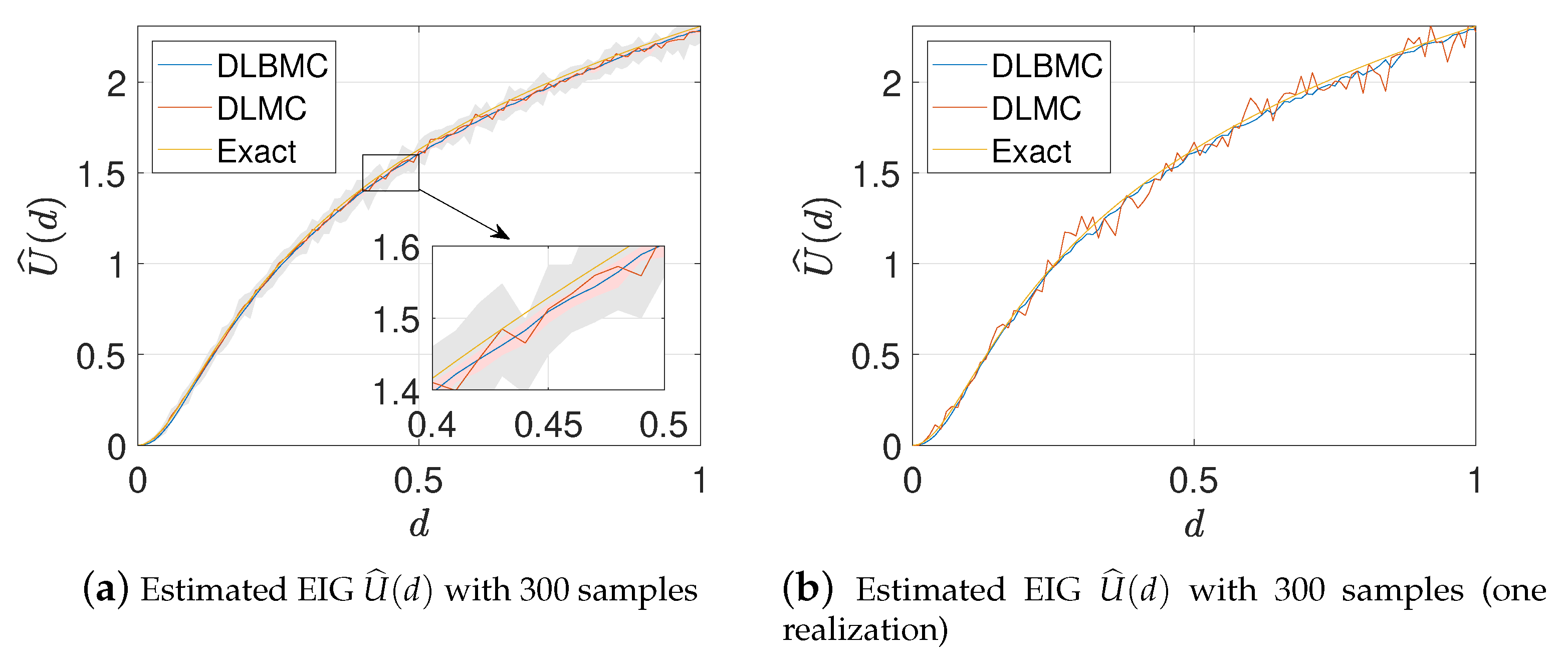
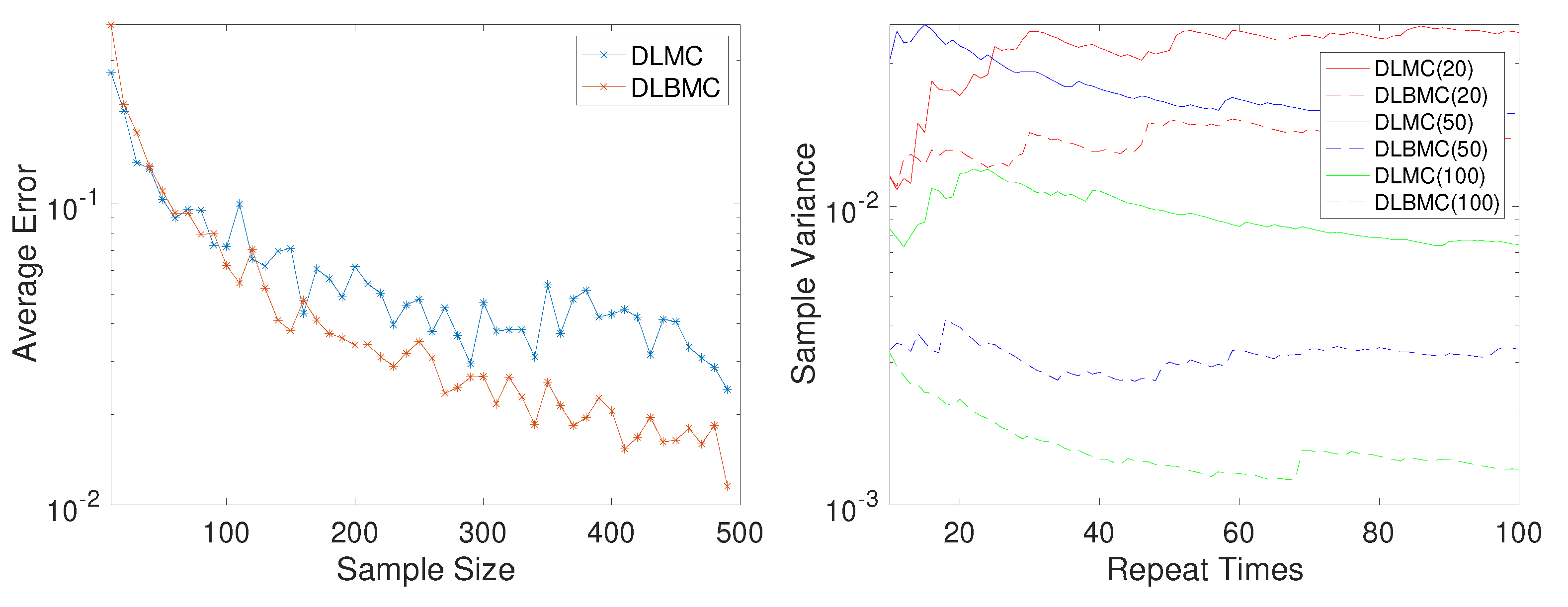
We consider the one-dimensional case where , , and set the standard deviation of the noise to . The hyperparameters of DLBMC are set to and Figure 1 shows the exact EIG, the estimated EIG using DLMC with 300 samples, and the estimated EIG using DLBMC with 300 samples. It can be seen that the estimated EIG of DLBMC is more accurate and more stable than that of DLMC. Besides, for , the relationship between the sample size and the bias of the DLMC and DLBMC estimators is studied. As the sample size increases, we compute the bias of the DLBMC estimator and the DLMC estimator averaging 20 trails respectively. Figure 2(Left) shows the results of the bias, where it can be seen that the DLBMC estimator converges to the true value faster than the DLMC estimator, and DLBMC is more accurate than DLMC.
As discussed in Section 3.2, the variance of the BMC estimator for the uniform distribution is not explicitly given. We use the sample variance as an alternative to compare the discrepancy of the DLMC estimator and the DLBMC estimator. Fixing the design point , for different sample sizes of DLMC and DLBMC, we repeatedly compute the estimator n times, and denote them by . Let denote the mean estimator, , and then the sample variance estimator is defined as
As the number of repeat times n increases, we compare the sample variance of two estimators with different sample sizes for DLMC and DLBMC in Figure 2(Right). It is clear that the DLBMC estimator outperforms the DLMC estimator.
4.2. Test Problem 2: Nonlinear Simple Problem
In this section, a simple nonlinear model is tested, which is also studied in [14]. This model is written as
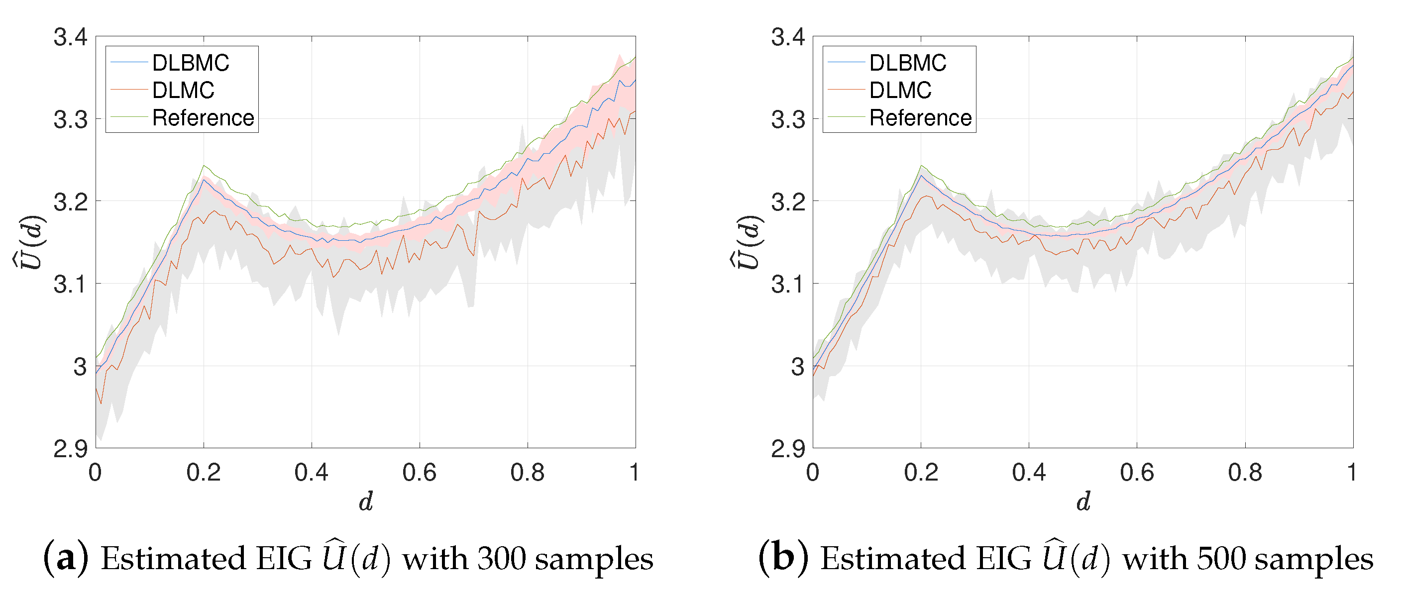
the prior is set to , and the standard deviation of the observation noise is set to . The hyperparameters of DLBMC are set to and
Figure 3a,b show the estimated EIG using DLMC and DLBMC with 300 and 500 samples respectively. A reference solution using DLMC with samples is also compared in Figure 3a,b. Here, 20 trails of the DLMC estimator and the DLBMC estimator are generated, and Figure 3 shows the mean estimates and the intervals containing 80% of the trails. It is clear that, compared to DLMC, our DLBMC estimator has smaller variances. Compared to the reference solution, DLBMC gives biased estimation. With the increasing sample size, the extent of bias is reduced as we expect.
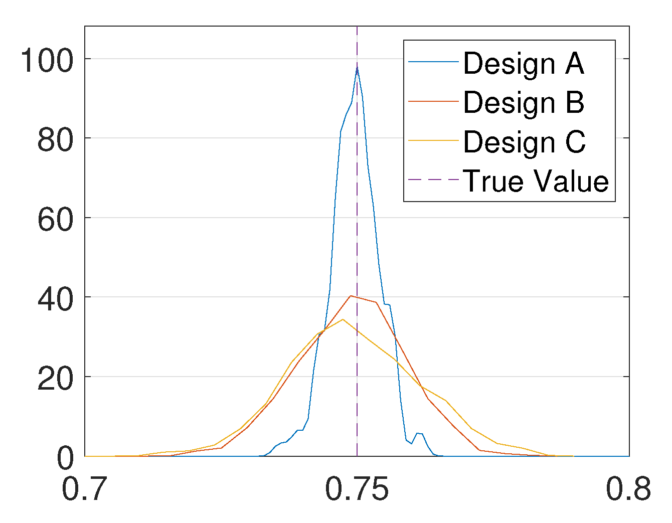
To illustrate the effect of optimal design, we compare the posterior distribution given by three design points. Let design A = 1 be the optimal design point, let design B = 0.2 be the local maximizer of the EIG, and let design C = 0 which has the least information since it has the least EIG value. The MH-MCMC algorithm (Algorithm A1) with and is used to generate samples of the posterior distribution, and kernel density estimation is used to obtain the posterior density functions from these samples. For this test problem, the ground-truth is set to 0.75. From Figure 4, it can be seen that the posterior distribution obtained through design A is the most accurate, and it has the smallest variance.
4.3. Test Problem 3: Source Inversion for the Diffusion Problem
Letting be a bounded and connected domain with a polygonal boundary , the governing equation of the diffusion problem studied in this test problem is: find a random function , such that -a.e. in ,
where is a probability space. We consider a square physical domain , and in (14)–(15) denotes the concentration of a contaminant at the point . Let denote the field of contaminant source. As f is usually strictly positive following the setting in [13,46,47,48], we set the prior distribution of to a log-normal random field, that is, where is a normal random field. In this study, the experimental goal is to infer the underlying contaminant field f given several observations , where design variable denotes i-th sensor placement, the response is the corresponding numerical PDE solution with additional noise, that is, , , and K is the number of sensors. In this test problem, the hyperparameters of DLBMC are set to and
We parameterize the permeability field by a truncated Karhunen-Loève (KL) expansion. Consider the random field with mean function , standard deviation and covariance function ,
where c is the correlation length. Then the truncated KL expansion of f is expressed as
where and are the eigenfunctions and eigenvalues of (16) and are uncorrelated random variables. The prior of are set to be independent standard normal distributions, for .
In the numerical experiment, we set , and . Fixing the hyperparameters in the truncated KL expansion, the response depends on the random variables . Therefore we define the parameter of interest as , and rewrite the governing diffusion equation as,
We use the bilinear finite element method (FEM) to discretize the diffusion equation over a square grid and let the standard deviation of noise be 1% of the mean observed value. Supposing K sensors are placed over the design space, generally, we can perform a batch design, and write the following altered forward model
where the subscript i denotes the i-th design variable for . Directly maximing over the EIG with altered forward model can give optimal design in the context of batch design.
Let denote the underlying true permeability field. Suppose we have collected data on K sensors, and then we perform MCMC to get samples of the posterior distribution using Algorithm A1. In this test problem, we set . Two useful statistics can be obtained from the samples—the maximum a posterior (MAP) estimate and the mean estimate . Let and be the source fields generated by and respectively. To test the accuracy of the inversion, we introduce the following relative errors
where and are discretized over the FEM grids for computational simplicity and denotes the vector norm.
Noting that performing grid search over grid is computationally expensive, we utilize Bayesian optimization method to efficiently find the optimal designs within a few iterations. Three cases of K are considered in the following, which are .
First, for , we first perform Bayesian optimization over a grid. The performance of Bayesian optimization is shown in Figure 5. In Figure 5(Left), we can see that, Bayesian optimization can find the maximum of the EIG within a few iterations. The optimal design found by Bayesian optimization is , which is expected due to the symmetry of the forward model. In this case, as the number of gird points (289 points) is not too large, we can verify that the optimal design is through grid search. Figure 5(Right) shows that the average cumulative regret is convergent to zero.
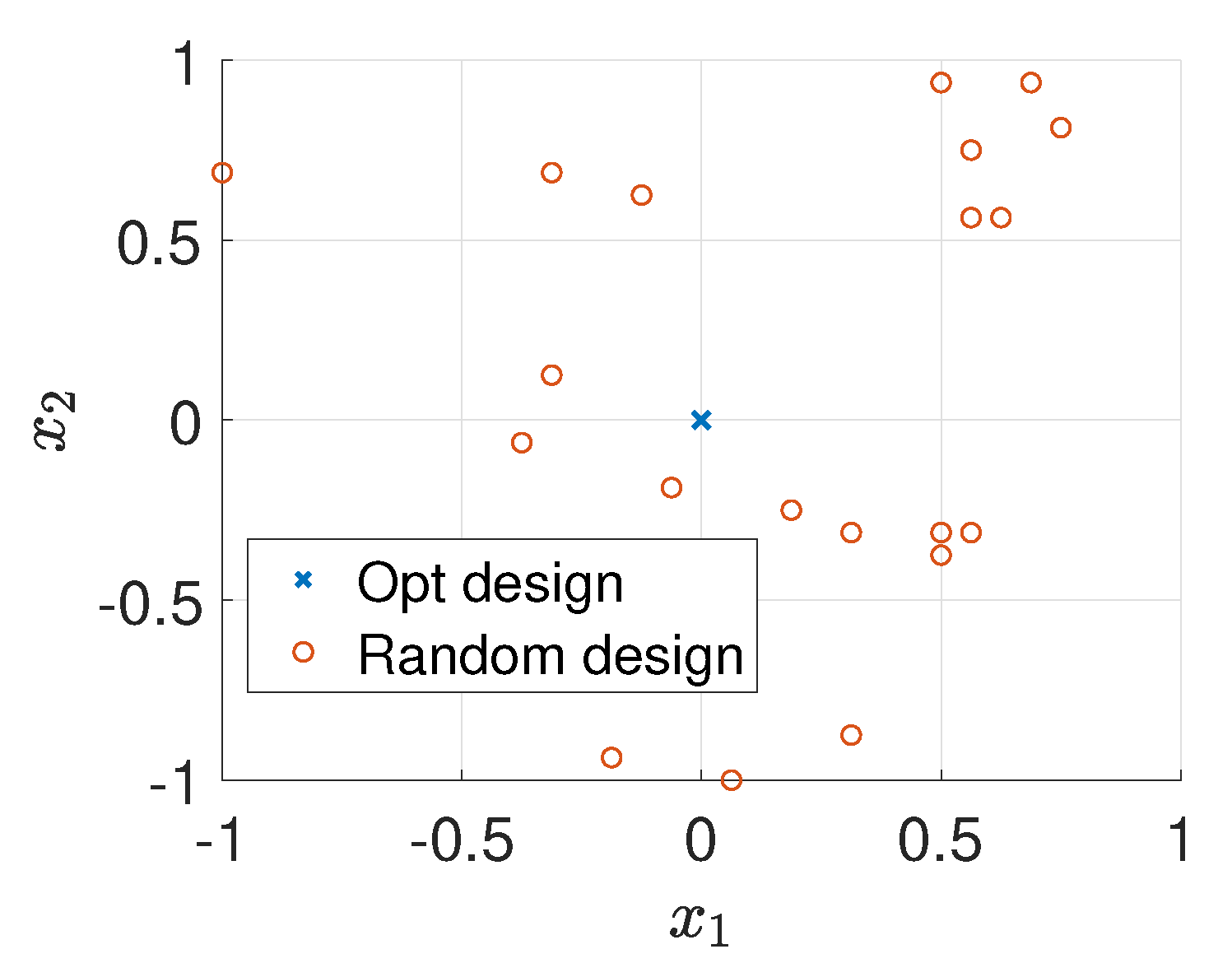
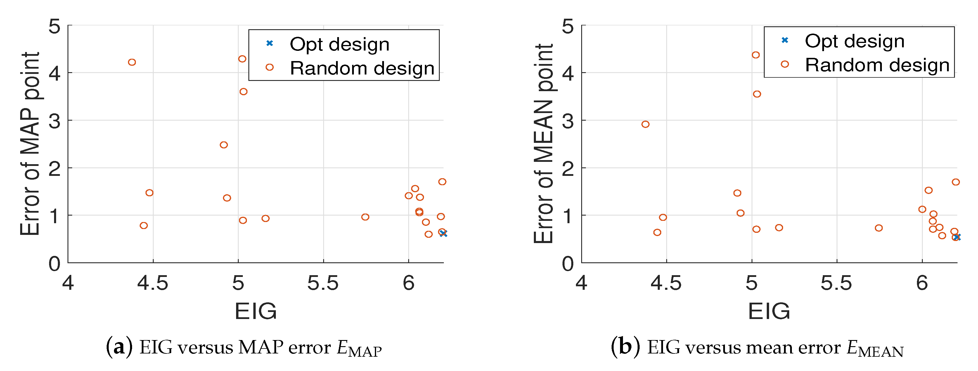
For comparison, we randomly generate 20 different design points and use the MH-MCMC algorithm to generate 4000 samples of the posterior distribution. Figure 6 shows the locations of the optimal design and the 20 random designs. Figure 7a,b show the relative errors of MAP and mean estimates of the source field (averaged over 20 trails) versus the values of EIG, where it is clear that as the value of EIG becomes larger, the errors of both MAP and mean estimates reduce. In addition, the optimal design point gives large EIG values and relatively small errors. Although the errors associated with the optimal design point are typically smaller than the errors associated with the random design points. They are still large, and the estimated source fields are not accurate enough. Therefore, we next consider more design points.
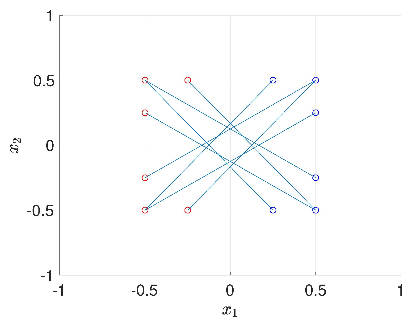
For the multiple design cases (), given the fact that the computational cost of batch design increases exponentially as K increases, we perform Bayesian optimization over a uniform coarse grid. For , it can be seen that the optimal solution is not unique due to the symmetry of the forward model, for example, and share the same EIG value. After performing Bayesian optimization several times with BO budget , the sets of optimal designs for case are shown in Figure 8, where each line connecting blue circle and red circle represents a pair of optimal design. The numerical result shows that, compared with a pair of two design points that are symmetric with respect to , a pair of slightly skewed design points can provide more information.
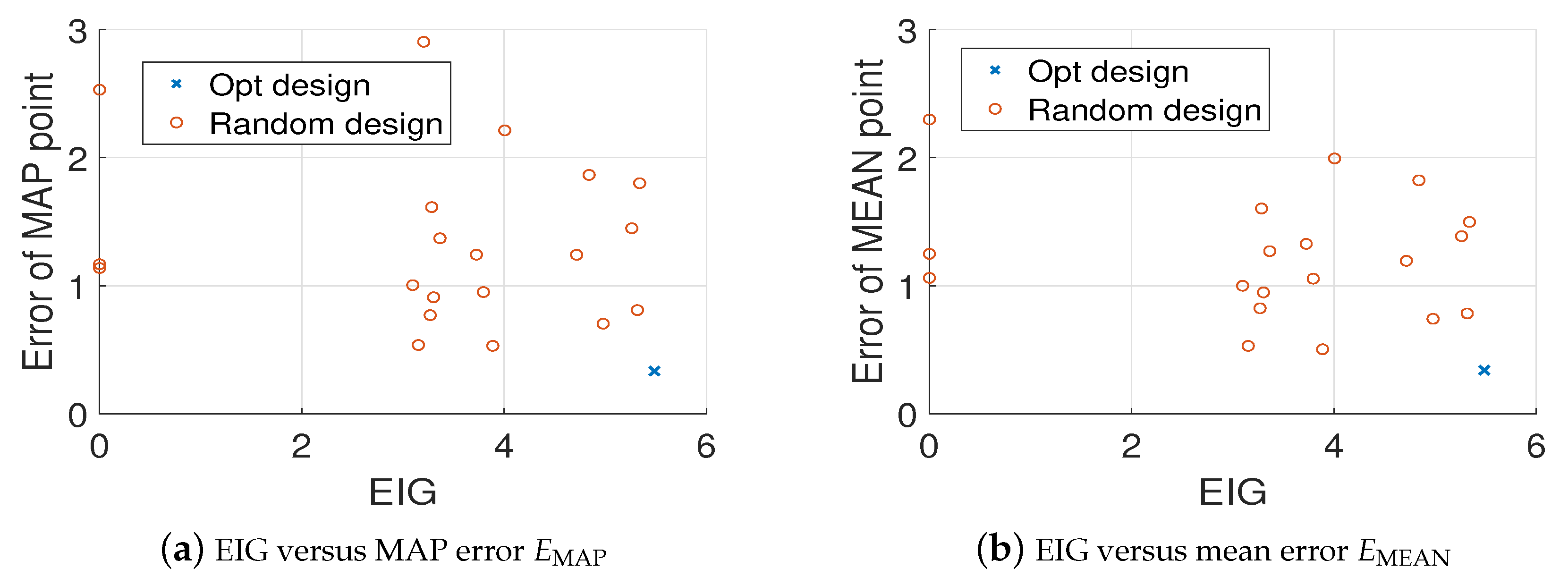
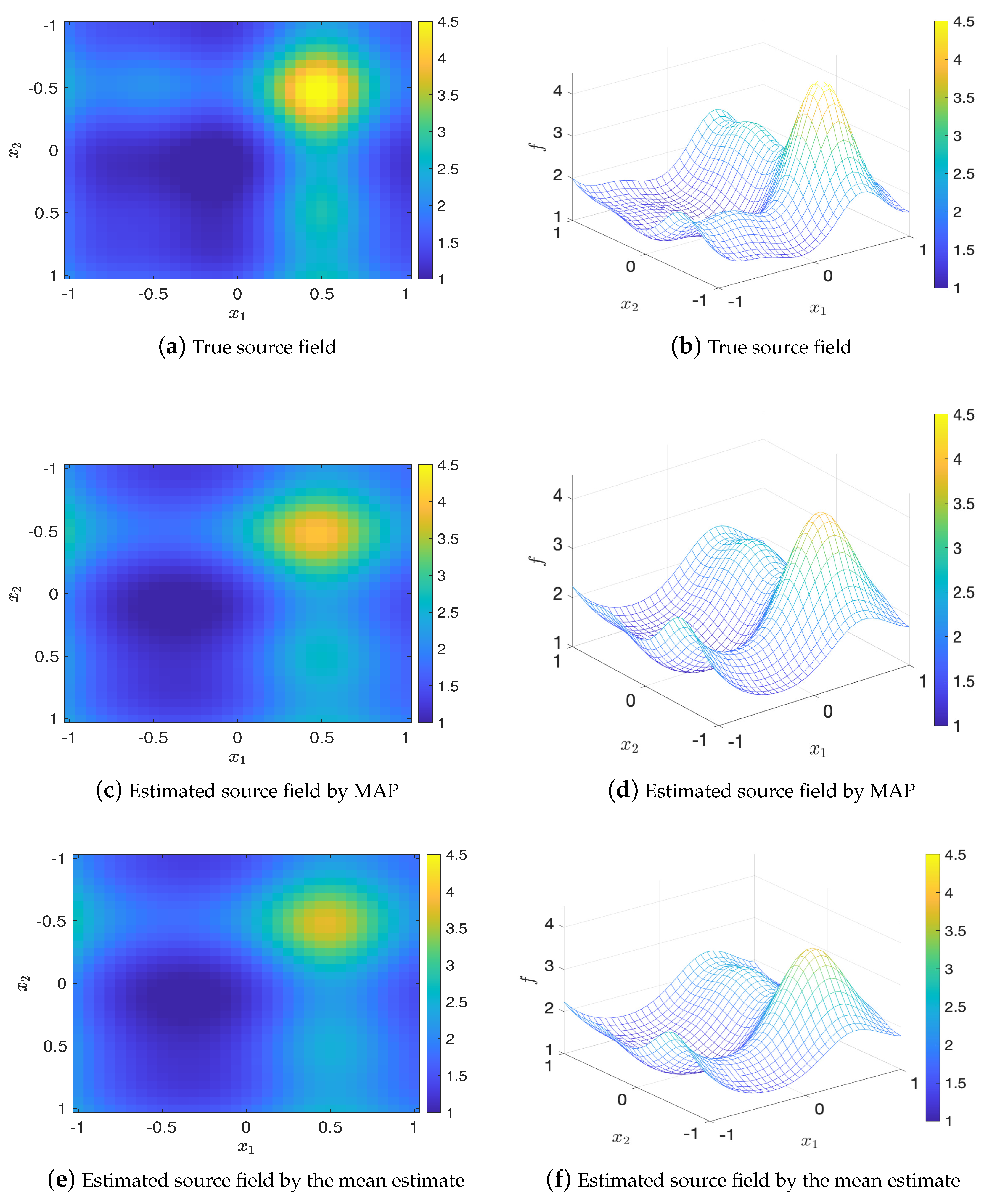
Again, we randomly generate 20 sets of design points, and compare them with the optimal design (we choose ). Figure 9 shows the errors of MAP and mean estimates (averaged over 20 trails) of the source field versus the values of EIG, where it is clear that the optimal design leads to the largest EIG value and the smallest error. Besides, the comparison of true source field and the fields generated by MAP and mean estimates are presented in Figure 10. It can be seen that the estimated source field associated with the optimal design matches the true source field well.
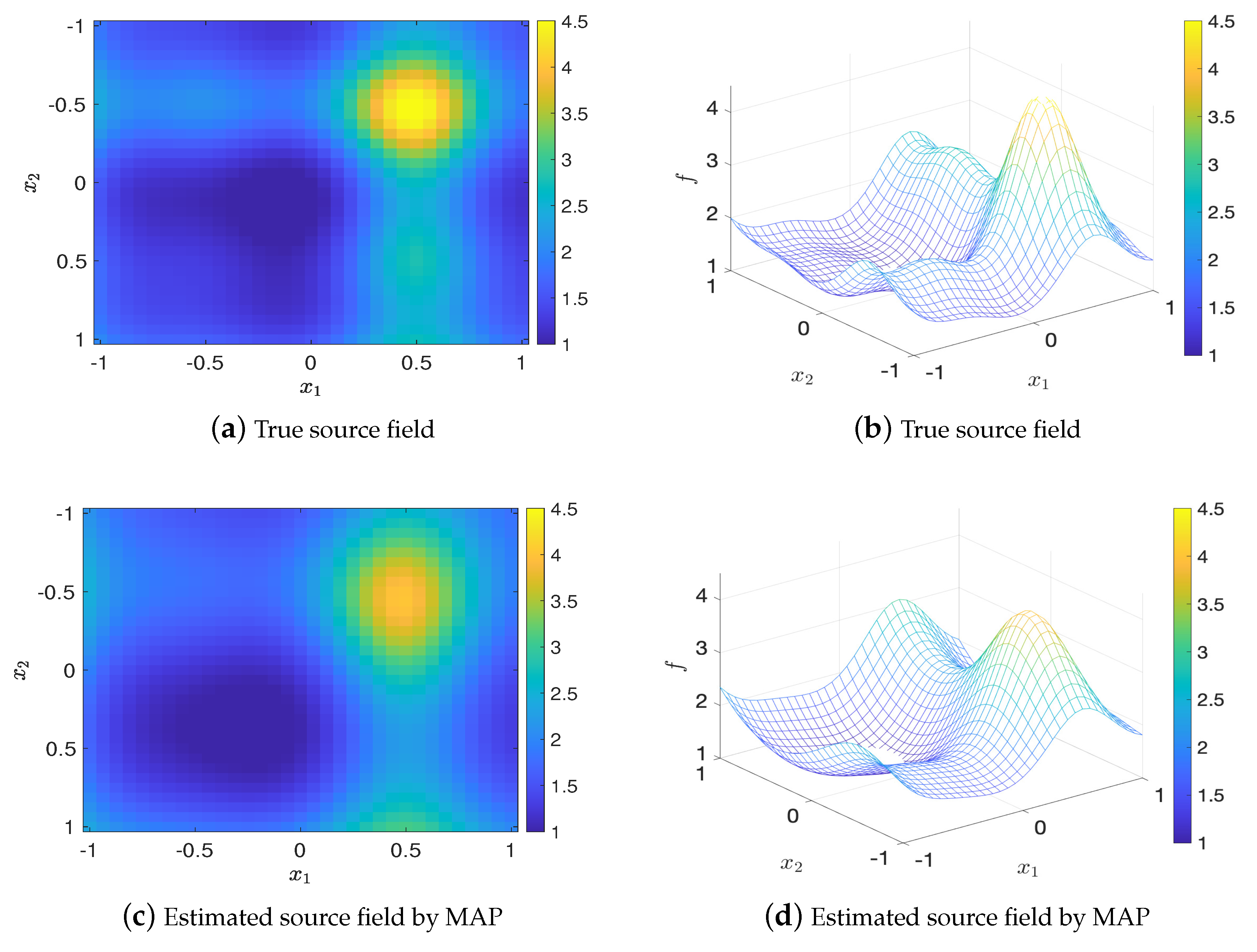
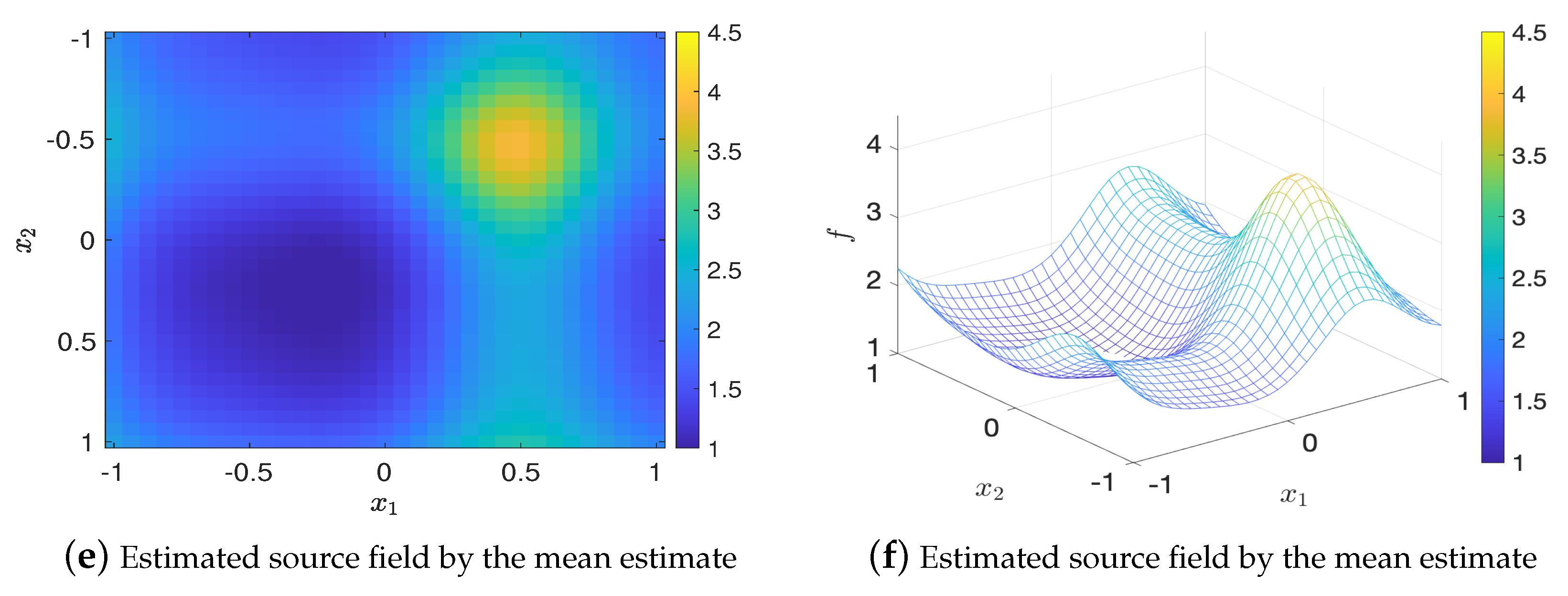
For , let the BO budget , the set of optimal design that found by Algorithm 2 is . Figure 11 shows the values of EIG and the relative errors in MAP and mean estimates (averaged over 20 trails) for the optimal design and twenty random designs, where it can be seen that the optimal design has the largest EIG value and the smallest errors which are consistent with the results for . Figure 12 shows that the estimated source fields generated by the MAP and the mean estimates match the true source field well.
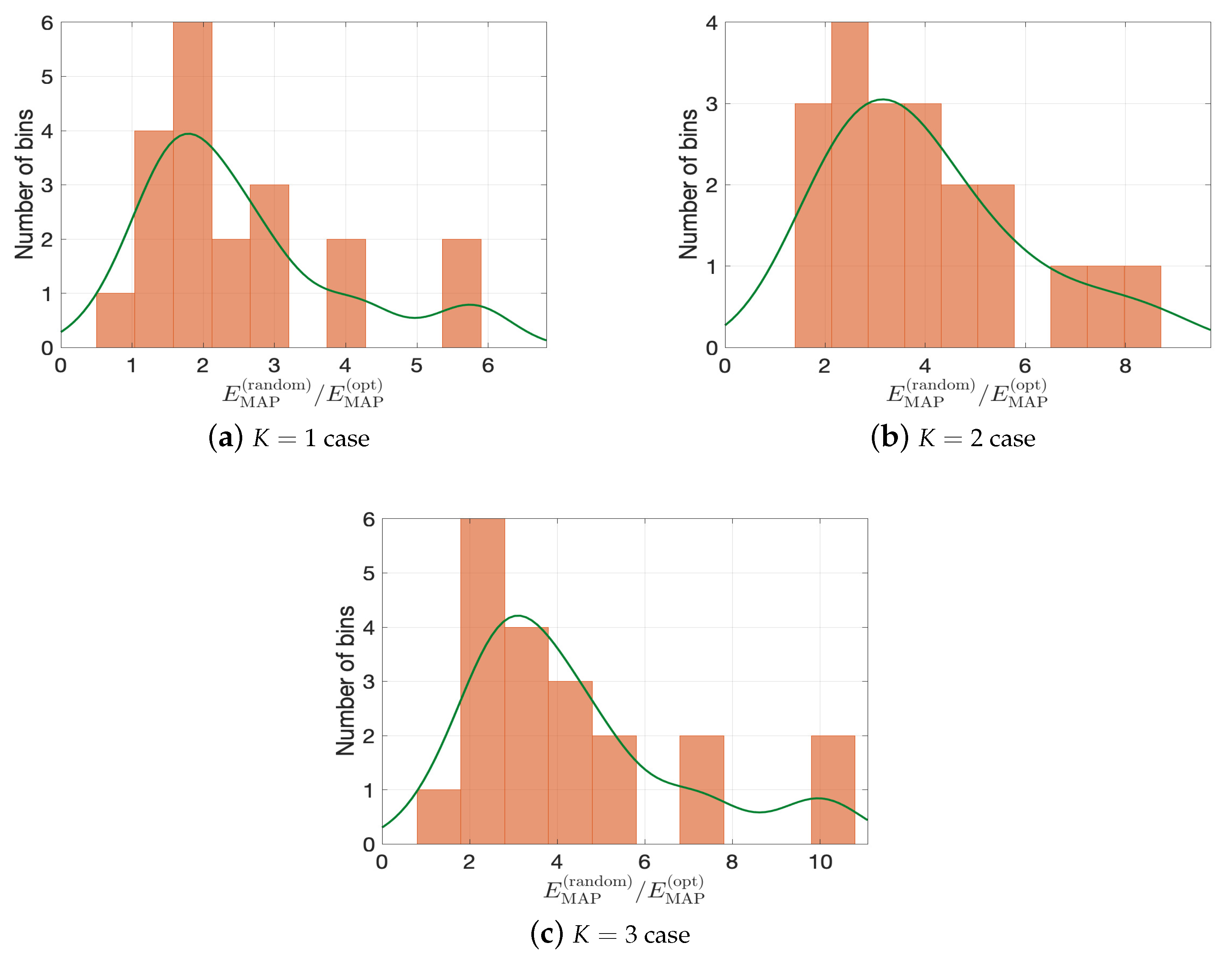
To further quantify the performance of optimal designs, we compute the ratio of of random designs and of optimal designs (denoted as and respectively) for cases. Figure 13 presents the histograms of ratio of relative errors (i.e., ), where the green lines are the corresponding kernel smoothing function estimates. We can see that, in all three cases, with high probability, the optimal design can give better posterior performance than the random designs. Especially, from Figure 13c, the error of random designs can be ten times greater than that of the optimal design.
5. Conclusions and Discussion
Efficiently using a small number of samples to reduce the cost of computing the expected information gain (EIG) is a fundamental concept to solve the challenging Bayesian optimal experimental design problem. Based on the Bayesian Monte Carlo (BMC) method, a novel double-loop Bayesian Monte Carlo (DLBMC) estimator is proposed for evaluating the EIG in this work. To result in an efficient overall optimization procedure to find the maximizer of the EIG, a Bayesian optimization (BO) procedure for EIG is developed. In addition, our analysis gives explicit expressions of the mean estimate of the BMC estimator and the bounds of its variance for the uniform and the normal distributions. Detailed numerical studies show that our DLBMC method can provide accurate mean estimates with small variances, and the overall BO procedure leads to optimal designs which give efficient Bayesian inference results.
As our novel DLBMC estimator for EIG is based on Gaussian process, it is currently limited to low-dimensional problems where the number of design variables is not large. In this work, the classical BO and MCMC approaches are used, and it is not straight forward to apply them for high-dimensional problems. For high-dimensional Bayesian optimal design problems with a large number of design variables, a possible solution is to conduct a sequential design procedure, and apply DLBMC at each step in the sequential procedure. Conducting a systematic DLBMC based on the sequential design will be the focus of our future work.
Author Contributions
Conceptualization, Z.X. and Q.L.; methodology, Q.L.; software, Z.X.; validation, Z.X.; formal analysis, Z.X.; investigation, Z.X.; resources, Z.X.; data curation, Z.X.; writing—original draft preparation, Z.X.; writing—review and editing, Q.L.; visualization, Z.X.; supervision, Q.L.; project administration, Q.L.; funding acquisition, Q.L. All authors have read and agreed to the published version of the manuscript.
Funding
This work is supported by the National Natural Science Foundation of China (No. 11601329).
Acknowledgments
The authors thank Jinglai Li for helpful discussions, and the anonymous reviewers for their thoughtful comments and suggestions that helped us improve our work and article.
Conflicts of Interest
The authors declare no conflict of interest.
Appendix A. Deduction of Linear Gaussian Model
We consider the standard linear Gaussian model,
where the noise and prior are assumed to be Gaussian, and .
then the likelihood is given by
The posterior is given by
where
By the definition of expected information gain,
Supposing , then we have
Thus,
Below, we show that
Let , which can be viewed as a linear transformation of a random vector. We have that , and the covariance of z is
Next, we consider the integration . Since ,
Therefore we have the analytical form of EIG,
Appendix B. Metropolis-Hastings MCMC Algorithm
| Algorithm A1 The Metropolis-Hastings Markov chain Monte Carlo (MH-MCMC) algorithm |
|
References
- Jones, M.; Goldstein, M.; Jonathan, P.; Randell, D. Bayes linear analysis for Bayesian optimal experimental design. J. Stat. Plan. Inference 2016, 171, 115–129. [Google Scholar] [CrossRef] [Green Version]
- Atkinson, A.; Donev, A.; Tobias, R. Optimum Experimental Designs, with SAS; Oxford University Press: Oxford, UK, 2007; Volume 34. [Google Scholar]
- Bernardo, J.M.; Smith, A.F. Bayesian Theory; John Wiley & Sons: Hoboken, NJ, USA, 2009; Volume 405. [Google Scholar]
- Stuart, A.M. Inverse problems: A Bayesian perspective. Acta Numer. 2010, 19, 451–559. [Google Scholar] [CrossRef] [Green Version]
- Tarantola, A. Inverse Problem Theory and Methods for Model Parameter Estimation; SIAM: Philadelphia, PA, USA, 2005; Volume 89. [Google Scholar]
- Kaipio, J.; Somersalo, E. Statistical and Computational Inverse Problems; Springer Science & Business Media: Berlin/Heidelberg, Germany, 2006; Volume 160. [Google Scholar]
- Alexanderian, A.; Petra, N.; Stadler, G.; Ghattas, O. A-optimal design of experiments for infinite-dimensional Bayesian linear inverse problems with regularized ℓ0-sparsification. SIAM J. Sci. Comput. 2014, 36, A2122–A2148. [Google Scholar] [CrossRef] [Green Version]
- Alexanderian, A.; Petra, N.; Stadler, G.; Ghattas, O. A fast and scalable method for A-optimal design of experiments for infinite-dimensional Bayesian nonlinear inverse problems. SIAM J. Sci. Comput. 2016, 38, A243–A272. [Google Scholar] [CrossRef] [Green Version]
- Weaver, B.P.; Williams, B.J.; Anderson-Cook, C.M.; Higdon, D.M. Computational enhancements to Bayesian design of experiments using Gaussian processes. Bayesian Anal. 2016, 11, 191–213. [Google Scholar] [CrossRef]
- Lindley, D.V. Bayesian Statistics, A Review; SIAM: Philadelphia, PA, USA, 1972; Volume 2. [Google Scholar]
- Chaloner, K.; Verdinelli, I. Bayesian experimental design: A review. Stat. Sci. 1995, 10, 273–304. [Google Scholar] [CrossRef]
- Müller, P.; Parmigiani, G. Optimal design via curve fitting of Monte Carlo experiments. J. Am. Stat. Assoc. 1995, 90, 1322–1330. [Google Scholar]
- Huan, X.; Marzouk, Y. Gradient-based stochastic optimization methods in Bayesian experimental design. Int. J. Uncertain. Quantif. 2014, 4, 479–510. [Google Scholar] [CrossRef]
- Huan, X.; Marzouk, Y.M. Simulation-based optimal Bayesian experimental design for nonlinear systems. J. Comput. Phys. 2013, 232, 288–317. [Google Scholar] [CrossRef] [Green Version]
- Wang, H.; Lin, G.; Li, J. Gaussian process surrogates for failure detection: A Bayesian experimental design approach. J. Comput. Phys. 2016, 313, 247–259. [Google Scholar] [CrossRef] [Green Version]
- Drovandi, C.C.; Tran, M.N. Improving the efficiency of fully Bayesian optimal design of experiments using randomised quasi-Monte Carlo. Bayesian Anal. 2018, 13, 139–162. [Google Scholar] [CrossRef] [Green Version]
- Feng, C.; Marzouk, Y.M. A layered multiple importance sampling scheme for focused optimal Bayesian experimental design. arXiv 2019, arXiv:1903.11187. [Google Scholar]
- Overstall, A.M.; Woods, D.C. Bayesian design of experiments using approximate coordinate exchange. Technometrics 2017, 59, 458–470. [Google Scholar] [CrossRef] [Green Version]
- Overstall, A.; McGree, J. Bayesian design of experiments for intractable likelihood models using coupled auxiliary models and multivariate emulation. Bayesian Anal. 2018, 15, 103–131. [Google Scholar] [CrossRef]
- Ryan, E.G.; Drovandi, C.C.; McGree, J.M.; Pettitt, A.N. A review of modern computational algorithms for Bayesian optimal design. Int. Stat. Rev. 2016, 84, 128–154. [Google Scholar] [CrossRef] [Green Version]
- Rasmussen, C.E. Gaussian processes in machine learning. In Summer School on Machine Learning; Springer: Berlin/Heidelberg, Germany, 2003; pp. 63–71. [Google Scholar]
- Deisenroth, M.P.; Huber, M.F.; Hanebeck, U.D. Analytic moment-based Gaussian process filtering. In Proceedings of the 26th Annual International Conference on Machine Learning, Montreal, QC, Canada, 14–18 June 2009; pp. 225–232. [Google Scholar]
- Santner, T.J.; Williams, B.J.; Notz, W.; Williams, B.J. The Design and Analysis of Computer Experiments; Springer: Berlin/Heidelberg, Germany, 2003; Volume 1. [Google Scholar]
- O’Hagan, A. Bayes–hermite quadrature. J. Stat. Plan. Inference 1991, 29, 245–260. [Google Scholar] [CrossRef]
- Rasmussen, C.E.; Ghahramani, Z. Bayesian Monte Carlo. In Proceedings of the 2003 Neural Information Processing Systems, Vancouver, BC, Canada, 8–13 December 2003; pp. 505–512. [Google Scholar]
- Briol, F.X.; Oates, C.J.; Girolami, M.; Osborne, M.A.; Sejdinovic, D. Probabilistic integration: A role in statistical computation? Stat. Sci. 2019, 34, 1–22. [Google Scholar] [CrossRef] [Green Version]
- Brochu, E.; Cora, V.M.; De Freitas, N. A tutorial on Bayesian optimization of expensive cost functions, with application to active user modeling and hierarchical reinforcement learning. arXiv 2010, arXiv:1012.2599. [Google Scholar]
- Snoek, J.; Larochelle, H.; Adams, R.P. Practical bayesian optimization of machine learning algorithms. In Proceedings of the 25th International Conference on Neural Information Processing Systems, Lake Tahoe, NV, USA, 3–6 December 2012; pp. 2951–2959. [Google Scholar]
- Shahriari, B.; Swersky, K.; Wang, Z.; Adams, R.P.; De Freitas, N. Taking the human out of the loop: A review of Bayesian optimization. Proc. IEEE 2015, 104, 148–175. [Google Scholar] [CrossRef] [Green Version]
- Ryan, K.J. Estimating expected information gains for experimental designs with application to the random fatigue-limit model. J. Comput. Graph. Stat. 2003, 12, 585–603. [Google Scholar] [CrossRef]
- Bungartz, H.J.; Griebel, M. Sparse grids. Acta Numer. 2004, 13, 147–269. [Google Scholar] [CrossRef]
- Xiu, D. Numerical Methods for Stochastic Computations: A Spectral Method Approach; Princeton University Press: Princeton, NJ, USA, 2010. [Google Scholar]
- Elman, H.; Liao, Q. Reduced Basis Collocation Methods for Partial Differential Equations with Random Coefficients. SIAM/ASA J. Uncertain. Quantif. 2013, 1, 192–217. [Google Scholar] [CrossRef] [Green Version]
- Villemonteix, J.; Vazquez, E.; Walter, E. An informational approach to the global optimization of expensive-to-evaluate functions. J. Glob. Optim. 2009, 44, 509. [Google Scholar] [CrossRef]
- Jones, D.R. A taxonomy of global optimization methods based on response surfaces. J. Glob. Optim. 2001, 21, 345–383. [Google Scholar] [CrossRef]
- Lam, R.; Willcox, K.; Wolpert, D.H. Bayesian optimization with a finite budget: An approximate dynamic programming approach. In Proceedings of the 2016 NIPS, Barcelona, Spain, 5–10 December 2016; pp. 883–891. [Google Scholar]
- Srinivas, N.; Krause, A.; Kakade, S.M.; Seeger, M. Gaussian process optimization in the bandit setting: No regret and experimental design. arXiv 2009, arXiv:0912.3995. [Google Scholar]
- Shahriari, B.; Bouchard-Côté, A.; Freitas, N. Unbounded Bayesian optimization via regularization. In Proceedings of the 19th International Conference on Artificial Intelligence and Statistics, Cadiz, Spain, 9–11 May 2016; pp. 1168–1176. [Google Scholar]
- Lizotte, D.J. Practical Bayesian Optimization. Ph.D. Thesis, University of Alberta, Edmonton, AB, Canada, 2008. [Google Scholar]
- Kushner, H.J. A new method of locating the maximum point of an arbitrary multipeak curve in the presence of noise. J. Basic Eng. Mar. 1964, 86, 97–106. [Google Scholar] [CrossRef]
- Mockus, J.; Tiesis, V.; Zilinskas, A. The application of bayesian methods for seeking the extremum. In Toward Global Optimization; North-Holand: Amsterdam, The Netherlands, 1978. [Google Scholar]
- Jones, D.R.; Schonlau, M.; Welch, W.J. Efficient global optimization of expensive black-box functions. J. Glob. Optim. 1998, 13, 455–492. [Google Scholar] [CrossRef]
- Metropolis, N.; Rosenbluth, A.W.; Rosenbluth, M.N.; Teller, A.H.; Teller, E. Equation of state calculations by fast computing machines. J. Chem. Phys. 1953, 21, 1087–1092. [Google Scholar] [CrossRef] [Green Version]
- Hastings, W.K. Monte Carlo sampling methods using Markov chains and their applications. Biometrika 1970, 57, 97–109. [Google Scholar] [CrossRef]
- Robert, C.; Casella, G. Monte Carlo Statistical Methods; Springer Science & Business Media: Berlin/Heidelberg, Germany, 2013. [Google Scholar]
- Marzouk, Y.M.; Najm, H.N.; Rahn, L.A. Stochastic spectral methods for efficient Bayesian solution of inverse problems. J. Comput. Phys. 2007, 224, 560–586. [Google Scholar] [CrossRef]
- Marzouk, Y.M.; Najm, H.N. Dimensionality reduction and polynomial chaos acceleration of Bayesian inference in inverse problems. J. Comput. Phys. 2009, 228, 1862–1902. [Google Scholar] [CrossRef] [Green Version]
- Li, J.; Marzouk, Y.M. Adaptive construction of surrogates for the Bayesian solution of inverse problems. SIAM J. Sci. Comput. 2014, 36, A1163–A1186. [Google Scholar] [CrossRef] [Green Version]
Figure 1.
Estimated expected information gain (EIG) profile over the design space for test problem 1. (a) Pink and gray shaded areas represent the interval containing 80% of 20 independent estimates of two estimators at each d respectively. Blue line and red line indicates the means of estimates. (b) One set of realizations of the two estimators.

Figure 2.
(Left) Error averaging over trails versus the sample size of DLMC and DLBMC. (Right) Sample variance versus the repeat times for different sample sizes of double-loop Monte Carlo (DLMC) and double-loop Bayesian Monte Carlo (DLBMC) (numbers in the parenthesis indicate the sample sizes).
Figure 2.
(Left) Error averaging over trails versus the sample size of DLMC and DLBMC. (Right) Sample variance versus the repeat times for different sample sizes of double-loop Monte Carlo (DLMC) and double-loop Bayesian Monte Carlo (DLBMC) (numbers in the parenthesis indicate the sample sizes).

Figure 3.
Estimated EIG profile over the design space for test problem 2. Pink and gray shaded areas represent the interval containing 80% of 20 independent estimates of EIG at each d for DLBMC and DLMC respectively. Blue line and red line denotes the means of these estimators. Green line denotes the reference solution given by DLMC with samples.

Figure 4.
Posterior density functions given by different designs.

Figure 5.
(Left) Maximum EIG value at iteration t of Bayesian optimization. (Right) Average cumulative regret at iteration t of Bayesian optimization. , test problem 3.
Figure 5.
(Left) Maximum EIG value at iteration t of Bayesian optimization. (Right) Average cumulative regret at iteration t of Bayesian optimization. , test problem 3.

Figure 6.
Sensor locations for , test problem 3.

Figure 7.
Value of EIG versus the relative errors averaged over 20 trails, , test problem 3.

Figure 8.
Optimal design (each line connecting blue circle and red circle represents a pair of optimal design points), , test problem 3.
Figure 8.
Optimal design (each line connecting blue circle and red circle represents a pair of optimal design points), , test problem 3.

Figure 9.
Value of EIG versus the relative errors averaged over 20 trails, , test problem 3.

Figure 10.
Comparison of the true source field and estimated source fields by MAP and mean estimates for , test problem 3.
Figure 10.
Comparison of the true source field and estimated source fields by MAP and mean estimates for , test problem 3.

Figure 11.
Value of EIG versus the relative errors averaged over 20 trails, , test problem 3.

Figure 12.
Comparison of the true source field and estimated source fields by MAP and mean estimates for , test problem 3.
Figure 12.
Comparison of the true source field and estimated source fields by MAP and mean estimates for , test problem 3.


Figure 13.
Histograms of . Green lines denotes the kernel smoothing function estimates.

© 2020 by the authors. Licensee MDPI, Basel, Switzerland. This article is an open access article distributed under the terms and conditions of the Creative Commons Attribution (CC BY) license (http://creativecommons.org/licenses/by/4.0/).
Share and Cite
MDPI and ACS Style
Xu, Z.; Liao, Q. Gaussian Process Based Expected Information Gain Computation for Bayesian Optimal Design. Entropy 2020, 22, 258. https://0-doi-org.brum.beds.ac.uk/10.3390/e22020258
AMA Style
Xu Z, Liao Q. Gaussian Process Based Expected Information Gain Computation for Bayesian Optimal Design. Entropy. 2020; 22(2):258. https://0-doi-org.brum.beds.ac.uk/10.3390/e22020258
Chicago/Turabian StyleXu, Zhihang, and Qifeng Liao. 2020. "Gaussian Process Based Expected Information Gain Computation for Bayesian Optimal Design" Entropy 22, no. 2: 258. https://0-doi-org.brum.beds.ac.uk/10.3390/e22020258
Note that from the first issue of 2016, this journal uses article numbers instead of page numbers. See further details here.