Using Matrix-Product States for Open Quantum Many-Body Systems: Efficient Algorithms for Markovian and Non-Markovian Time-Evolution


Abstract
:1. Introduction
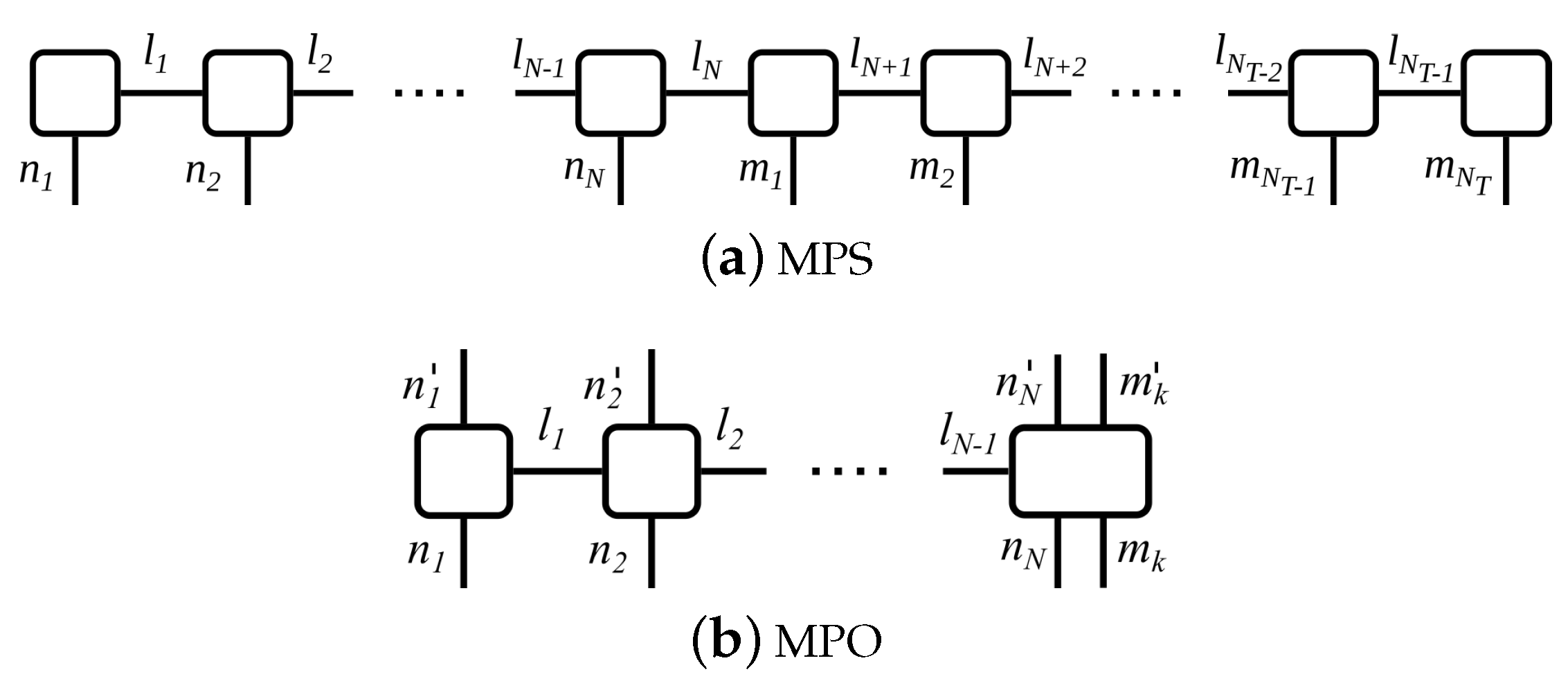
2. Time Evolution with Matrix-Product States
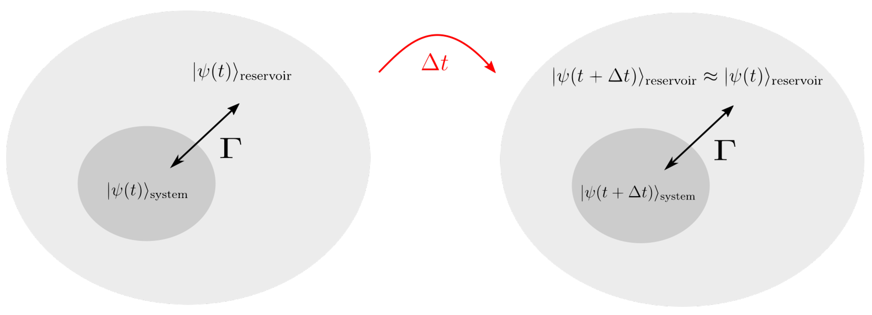
3. Modeling Markovian System–Reservoir Interaction
3.1. Model
3.2. Quantum Stochastic Schrödinger Equation (QSSE)
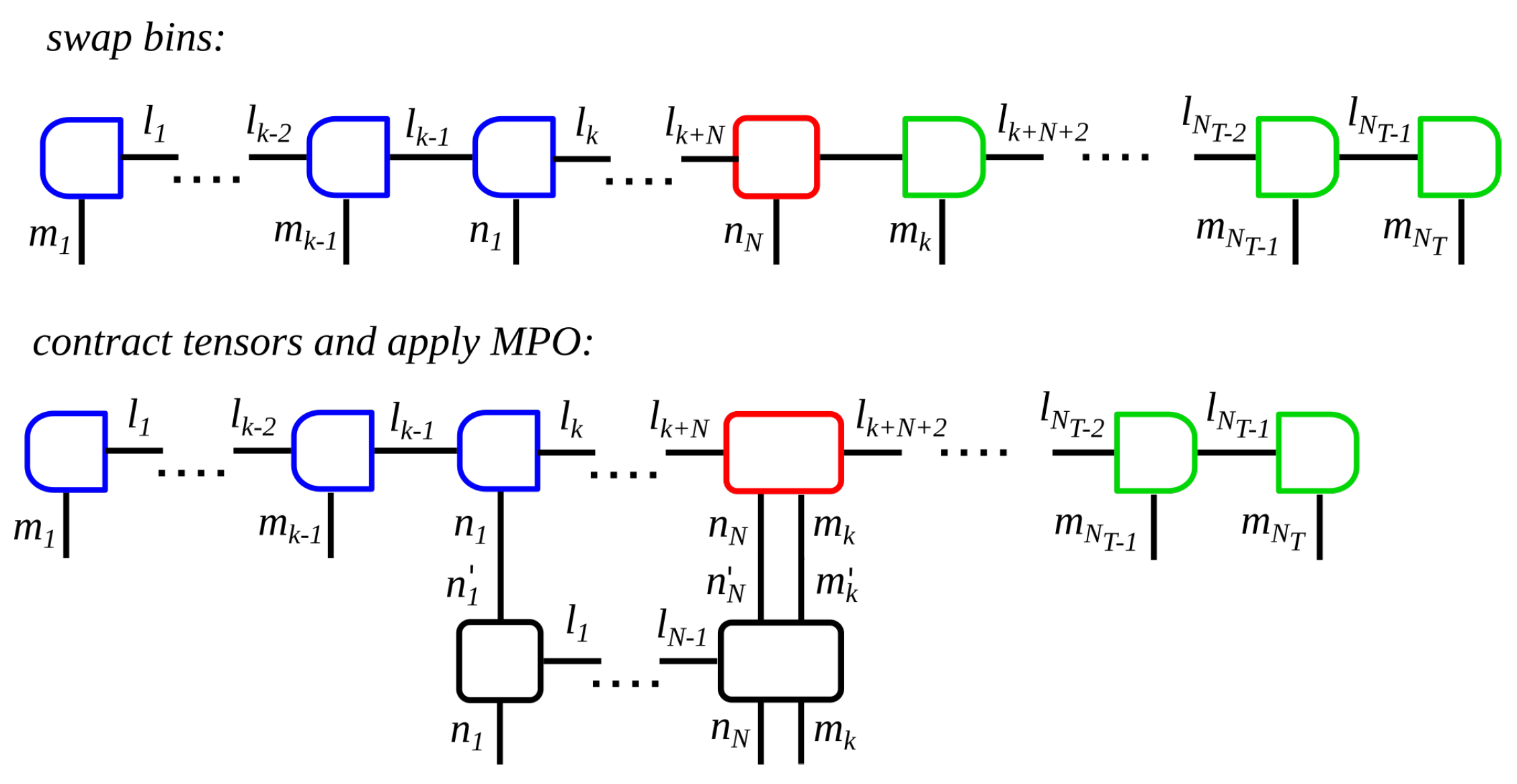
3.3. Algorithm
4. Modeling Non-Markovian System—Reservoir Interaction
4.1. Model
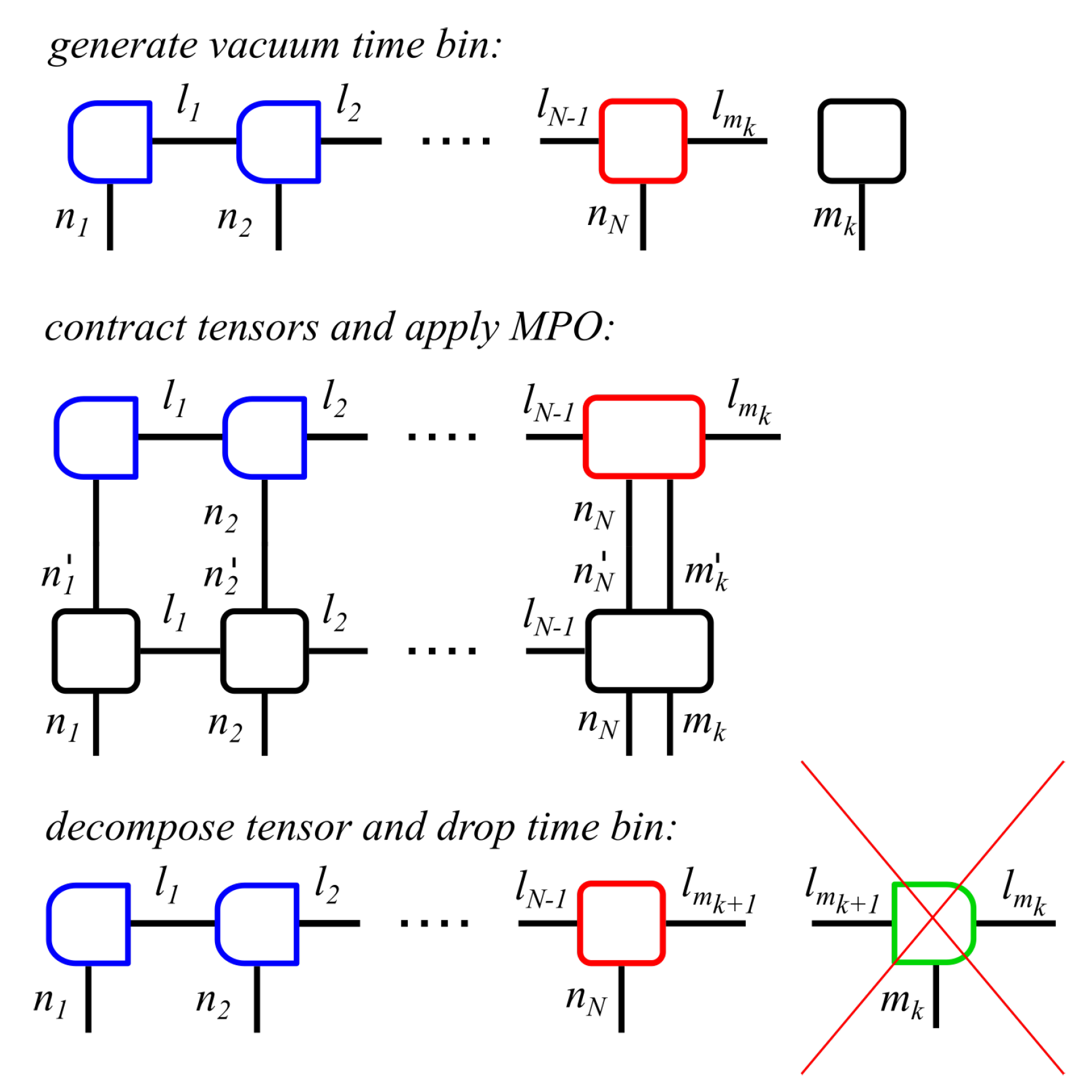
4.2. Algorithm
5. Application Examples
5.1. A Dissipative Spin Chain with Markovian Interaction
5.2. An Open Spin Chain in a Semi-Infinite Waveguide
6. Conclusions
Author Contributions
Funding
Conflicts of Interest
References
- Breuer, H.P.; Petruccione, F.F. The Theory of Open Quantum Systems; Oxford University Press: Oxford, UK, 2002. [Google Scholar]
- Crispin Gardiner, P.Z. Quantum Noise—A Handbook of Markovian and Non-Markovian Quantum Stochastic Methods with Applications to Quantum Optics; Springer Verlag: Berlin, Germany, 2002. [Google Scholar]
- Carmichael, H. An Open Systems Approach to Quantum Optics; Springer: Berlin, Germany, 1993. [Google Scholar]
- Weiss, U. Quantum Dissipative Systems, 4th ed.; World Scientific Publishing Co.: Singapore, 2012. [Google Scholar]
- Nielsen, M.A.; Chuang, I.L. Quantum Computation and Quantum Information; Cambridge University Press: Cambridge, UK, 2010. [Google Scholar]
- de Vega, I.; Porras, D.; Ignacio Cirac, J. Matter-Wave Emission in Optical Lattices: Single Particle and Collective Effects. Phys. Rev. Lett. 2008, 101, 260404. [Google Scholar] [CrossRef] [PubMed]
- Navarrete-Benlloch, C.; de Vega, I.; Porras, D.; Cirac, J.I. Simulating quantum-optical phenomena with cold atoms in optical lattices. New J. Phys. 2011, 13, 023024. [Google Scholar] [CrossRef] [Green Version]
- Häffner, H.; Roos, C.; Blatt, R. Quantum computing with trapped ions. Phys. Rep. 2008, 469, 155–203. [Google Scholar] [CrossRef] [Green Version]
- Blatt, R.; Wineland, D. Entangled states of trapped atomic ions. Nature 2008, 453, 1008–1015. [Google Scholar] [CrossRef]
- Rotter, I.; Bird, J.P. A review of progress in the physics of open quantum systems: Theory and experiment. Rep. Prog. Phys. 2015, 78, 114001. [Google Scholar] [CrossRef]
- Nogues, G.; Rauschenbeutel, A.; Osnaghi, S.; Brune, M.; Raimond, J.M.; Haroche, S. Seeing a single photon without destroying it. Nature 1999, 400, 239–242. [Google Scholar] [CrossRef]
- Prokof, N.V.; Stamp, P.C.E. Giant spins and topological decoherence: A Hamiltonian approach. J. Condens. Matter Phys. 1993, 5, L663–L670. [Google Scholar] [CrossRef]
- Lambert, N.; Chen, Y.N.; Cheng, Y.C.; Li, C.M.; Chen, G.Y.; Nori, F. Quantum biology. Nat. Phys. 2013, 9, 10–18. [Google Scholar] [CrossRef]
- Daley, A. Quantum trajectories and open many-body quantum systems. Adv. Phys. 2014, 63, 77–149. [Google Scholar] [CrossRef] [Green Version]
- de Vega, I.; Alonso, D. Dynamics of non-Markovian open quantum systems. Rev. Mod. Phys. 2017, 89, 015001. [Google Scholar] [CrossRef] [Green Version]
- Koch, C.P. Controlling open quantum systems: Tools, achievements, and limitations. J. Condens. Matter Phys. 2016, 28, 213001. [Google Scholar] [CrossRef] [PubMed] [Green Version]
- Cirac, J.I.; Zoller, P. Goals and opportunities in quantum simulation. Nat. Phys. 2012, 8, 264–266. [Google Scholar] [CrossRef]
- Droenner, L.; Carmele, A. Boundary-driven Heisenberg chain in the long-range interacting regime: Robustness against far-from-equilibrium effects. Phys. Rev. B 2017, 96, 184421. [Google Scholar] [CrossRef] [Green Version]
- Žnidarič, M.; Scardicchio, A.; Varma, V.K. Diffusive and Subdiffusive Spin Transport in the Ergodic Phase of a Many-Body Localizable System. Phys. Rev. Lett. 2016, 117, 040601. [Google Scholar] [CrossRef] [PubMed] [Green Version]
- Heyl, M.; Polkovnikov, A.; Kehrein, S. Dynamical Quantum Phase Transitions in the Transverse-Field Ising Model. Phys. Rev. Lett. 2013, 110, 135704. [Google Scholar] [CrossRef] [PubMed]
- Huber, J.; Kirton, P.; Rabl, P. Non-equilibrium magnetic phases in spin lattices with gain and loss. arXiv 2019, arXiv:1908.02290. [Google Scholar]
- Huber, J.; Rabl, P. Active energy transport and the role of symmetry breaking in microscopic power grids. Phys. Rev. A 2019, 100, 012129. [Google Scholar] [CrossRef] [Green Version]
- Pizzi, A.; Nunnenkamp, A.; Knolle, J. Bistability and time crystals in long-ranged directed percolation. arXiv 2020, arXiv:2004.13034. [Google Scholar]
- Bertini, B.; Heidrich-Meisner, F.; Karrasch, C.; Prosen, T.; Steinigeweg, R.; Znidaric, M. Finite-temperature transport in one-dimensional quantum lattice models. arXiv 2020, arXiv:2003.03334. [Google Scholar]
- Hauke, P.; Tagliacozzo, L. Spread of Correlations in Long-Range Interacting Quantum Systems. Phys. Rev. Lett. 2013, 111, 207202. [Google Scholar] [CrossRef]
- Trautmann, N.; Hauke, P. Trapped-ion quantum simulation of excitation transport: Disordered, noisy, and long-range connected quantum networks. Phys. Rev. A 2018, 97, 023606. [Google Scholar] [CrossRef] [Green Version]
- Prosen, T.C.V. Exact Nonequilibrium Steady State of a Strongly Driven Open XXZ Chain. Phys. Rev. Lett. 2011, 107, 137201. [Google Scholar] [CrossRef] [PubMed] [Green Version]
- Ljubotina, M.; Žnidari, M.; Prosen, T. Spin diffusion from an inhomogeneous quench in an integrable system. Nat. Commun. 2017, 8, 16117. [Google Scholar] [CrossRef] [Green Version]
- Lange, F.; Ejima, S.; Shirakawa, T.; Yunoki, S.; Fehske, H. Spin transport through a spin-1/2 XXZ chain contacted to fermionic leads. Phys. Rev. B 2018, 97, 245124. [Google Scholar] [CrossRef] [Green Version]
- Žnidarič, M. Spin Transport in a one-dimensional anisotropic Heisenberg model. Phys. Rev. Lett. 2011, 106, 220601. [Google Scholar] [CrossRef] [PubMed]
- Žnidarič, M. Transport in a one-dimensional isotropic Heisenberg model at high temperature. J. Stat. Mech. Theory Exp. 2011, 2011, P12008. [Google Scholar] [CrossRef] [Green Version]
- Katzer, M.; Knorr, W.; Finsterhölzl, R.; Carmele, A. Long-range interaction in an open boundary-driven Heisenberg spin lattice—A far-from-equilibrium transition to ballistic transport. arXiv 2020, arXiv:2004.12738. [Google Scholar] [CrossRef]
- Wang, T.; Wang, X.; Sun, Z. Entanglement oscillations in open Heisenberg chains. Phys. A 2007, 383, 316–324. [Google Scholar] [CrossRef] [Green Version]
- Wu, Y.Z.; Ren, J.; Jiang, X.F. Dynamics of entanglement in Heisenberg chains with asymmetric DzyaloShinskii-moriya interactions. Int. J. Quantum Inf. 2011, 09, 751–761. [Google Scholar] [CrossRef]
- Lindblad, G. On the generators of quantum dynamical semigroups. Comm. Math. Phys. 1976, 48, 119–130. [Google Scholar] [CrossRef]
- Pollet, L. Recent developments in quantum Monte Carlo simulations with applications for cold gases. Rep. Prog. Phys. 2012, 75, 094501. [Google Scholar] [CrossRef] [PubMed]
- Kimble, H.J.; Dagenais, M.; Mandel, L. Photon Antibunching in Resonance Fluorescence. Phys. Rev. Lett. 1977, 39, 691–695. [Google Scholar] [CrossRef] [Green Version]
- Dalibard, J.; Castin, Y.; Mølmer, K. Wave-function approach to dissipative processes in quantum optics. Phys. Rev. Lett. 1992, 68, 580–583. [Google Scholar] [CrossRef] [PubMed] [Green Version]
- Dum, R.; Zoller, P.; Ritsch, H. Monte Carlo simulation of the atomic master equation for spontaneous emission. Phys. Rev. A 1992, 45, 4879–4887. [Google Scholar] [CrossRef]
- Zoller, P.; Gardiner, C.W. Quantum Noise in Quantum Optics: The Stochastic Schrödinger Equation. arXiv 1997, arXiv:quant-ph/9702030. [Google Scholar]
- Alonso, D.; de Vega, I. Multiple-Time Correlation Functions for Non-Markovian Interaction: Beyond the Quantum Regression Theorem. Phys. Rev. Lett. 2005, 94, 200403. [Google Scholar] [CrossRef] [Green Version]
- Piilo, J.; Maniscalco, S.; Härkönen, K.; Suominen, K.A. Non-Markovian Quantum Jumps. Phys. Rev. Lett. 2008, 100, 180402. [Google Scholar] [CrossRef] [Green Version]
- Pichler, H.; Zoller, P. Photonic Circuits with Time Delays and Quantum Feedback. Phys. Rev. Lett. 2016, 116, 093601. [Google Scholar] [CrossRef] [Green Version]
- Heisenberg, W. Zur Theorie des Ferromagnetismus. Z. Phys. 1928, 49, 619–636. [Google Scholar] [CrossRef]
- Bethe, H. Zur Theorie der Metalle—I. Eigenwerte und Eigenfunktionen der linearen Atomkette. Zeitschrift für Physik 1931, 71, 205–226. [Google Scholar] [CrossRef]
- Dupont, M.; Moore, J.E. Universal spin dynamics in infinite-temperature one-dimensional quantum magnets. Phys. Rev. B 2020, 101, 121106. [Google Scholar] [CrossRef] [Green Version]
- Hild, S.; Fukuhara, T.; Schauß, P.; Zeiher, J.; Knap, M.; Demler, E.; Bloch, I.; Gross, C. Far-from-Equilibrium Spin Transport in Heisenberg Quantum Magnets. Phys. Rev. Lett. 2014, 113, 147205. [Google Scholar] [CrossRef] [PubMed]
- Tang, Y.; Kao, W.; Li, K.Y.; Seo, S.; Mallayya, K.; Rigol, M.; Gopalakrishnan, S.; Lev, B.L. Thermalization near Integrability in a Dipolar Quantum Newton’s Cradle. Phys. Rev. X 2018, 8, 021030. [Google Scholar] [CrossRef] [Green Version]
- Langen, T.; Erne, S.; Geiger, R.; Rauer, B.; Schweigler, T.; Kuhnert, M.; Rohringer, W.; Mazets, I.E.; Gasenzer, T.; Schmiedmayer, J. Experimental observation of a generalized Gibbs ensemble. Science 2015, 348, 207–211. [Google Scholar] [CrossRef] [PubMed] [Green Version]
- Kinoshita, T.; Wenger, T.; Weiss, D.S. A quantum Newton’s cradle. Nature 2006, 440, 900–903. [Google Scholar] [CrossRef]
- Maier, C.; Brydges, T.; Jurcevic, P.; Trautmann, N.; Hempel, C.; Lanyon, B.P.; Hauke, P.; Blatt, R.; Roos, C.F. Environment-Assisted Quantum Transport in a 10-qubit Network. Phys. Rev. Lett. 2019, 122, 050501. [Google Scholar] [CrossRef] [PubMed] [Green Version]
- Derrida, B.; Evans, M.R.; Hakim, V.; Pasquier, V. Exact solution of a 1D asymmetric exclusion model using a matrix formulation. J. Phys. A Math. Theor. 1993, 26, 1493–1517. [Google Scholar] [CrossRef]
- Fannes, M.; Nachtergaele, B.; Werner, R.F. Finitely correlated states on quantum spin chains. Comm. Math. Phys. 1992, 144, 443–490. [Google Scholar] [CrossRef]
- Kolezhuk, A.K.; Mikeska, H.J. Finitely Correlated Generalized Spin Ladders. Int. J. Mod. Phys. B 1998, 12, 2325–2348. [Google Scholar] [CrossRef] [Green Version]
- Schollwöck, U. The density-matrix renormalization group. Rev. Mod. Phys. 2005, 77, 259–315. [Google Scholar] [CrossRef] [Green Version]
- Schollwöck, U. The density-matrix renormalization group in the age of matrix product states. Ann. Phys. N. Y. 2011, 326, 96–192. [Google Scholar] [CrossRef] [Green Version]
- White, S.R. Density-matrix algorithms for quantum renormalization groups. Phys. Rev. B 1993, 48, 10345–10356. [Google Scholar] [CrossRef] [PubMed]
- Vidal, G. Efficient Classical Simulation of Slightly Entangled Quantum Computations. Phys. Rev. Lett. 2003, 91, 147902. [Google Scholar] [CrossRef] [PubMed] [Green Version]
- Vidal, G. Efficient Simulation of One-Dimensional Quantum Many-Body Systems. Phys. Rev. Lett. 2004, 93, 040502. [Google Scholar] [CrossRef] [PubMed] [Green Version]
- White, S.R.; Feiguin, A.E. Real-Time Evolution Using the Density Matrix Renormalization Group. Phys. Rev. Lett. 2004, 93, 076401. [Google Scholar] [CrossRef] [PubMed] [Green Version]
- Orús, R.; Vidal, G. Infinite time-evolving block decimation algorithm beyond unitary evolution. Phys. Rev. B 2008, 78, 155117. [Google Scholar] [CrossRef] [Green Version]
- Suzuki, M. Relationship between d-Dimensional Quantal Spin Systems and (d+1)-Dimensional Ising Systems: Equivalence, Critical Exponents and Systematic Approximants of the Partition Function and Spin Correlations. Prog. Theor. Phys. 1976, 56, 1454–1469. [Google Scholar] [CrossRef]
- Suzuki, M. General theory of fractal path integrals with applications to many-body theories and statistical physics. J. Math. Phys. 1991, 32, 400–407. [Google Scholar] [CrossRef]
- Paeckel, S.; Köhler, T.; Swoboda, A.; Manmana, S.R.; Schollwöck, U.; Hubig, C. Time-evolution methods for matrix-product states. Ann. Phys. 2019, 411, 167998. [Google Scholar] [CrossRef]
- Benenti, G.; Casati, G.; Prosen, T.; Rossini, D. Negative differential conductivity in far-from-equilibrium quantum spin chains. EPL 2009, 85, 37001. [Google Scholar] [CrossRef] [Green Version]
- Prosen, T. Matrix product solutions of boundary driven quantum chains. J. Phys. A Math. Theor. 2015, 48, 373001. [Google Scholar] [CrossRef] [Green Version]
- Prosen, T.; Žnidarič, M. Matrix product simulations of non-equilibrium steady states of quantum spin chains. J. Stat. Mech. Theory Exp. 2009, 2009, P02035. [Google Scholar] [CrossRef] [Green Version]
- Karevski, D.; Popkov, V.; Schütz, G.M. Exact Matrix Product Solution for the Boundary-Driven Lindblad XXZ Chain. Phys. Rev. Lett. 2013, 110, 047201. [Google Scholar] [CrossRef] [Green Version]
- Cai, Z.; Barthel, T. Algebraic versus Exponential Decoherence in Dissipative Many-Particle Systems. Phys. Rev. Lett. 2013, 111, 150403. [Google Scholar] [CrossRef] [PubMed] [Green Version]
- Xu, X.; Guo, C.; Poletti, D. Interplay of interaction and disorder in the steady state of an open quantum system. Phys. Rev. B 2018, 97, 140201. [Google Scholar] [CrossRef] [Green Version]
- Mendoza-Arenas, J.J.; Žnidarič, M.; Varma, V.K.; Goold, J.; Clark, S.R.; Scardicchio, A. Asymmetry in energy versus spin transport in certain interacting disordered systems. Phys. Rev. B 2019, 99, 094435. [Google Scholar] [CrossRef] [Green Version]
- Popkov, V.; Prosen, T.C.V.; Zadnik, L. Inhomogeneous matrix product ansatz and exact steady states of boundary-driven spin chains at large dissipation. Phys. Rev. E 2020, 101, 042122. [Google Scholar] [CrossRef] [PubMed] [Green Version]
- Mascarenhas, E.; Flayac, H.; Savona, V. Matrix-product-operator approach to the nonequilibrium steady state of driven-dissipative quantum arrays. Phys. Rev. A 2015, 92, 022116. [Google Scholar] [CrossRef] [Green Version]
- Strathearn, A.; Kirton, P.; Kilda, D.; Keeling, J.; Lovett, B.W. Efficient non-Markovian quantum dynamics using time-evolving matrix product operators. Nat. Commun. 2018, 9, 3322. [Google Scholar] [CrossRef]
- Droenner, L.; Naumann, N.L.; Schöll, E.; Knorr, A.; Carmele, A. Quantum Pyragas control: Selective control of individual photon probabilities. Phys. Rev. A 2019, 99, 023840. [Google Scholar] [CrossRef] [Green Version]
- Carmele, A.; Nemet, N.; Canela, V.; Parkins, S. Pronounced non-Markovian features in multiply excited, multiple emitter waveguide QED: Retardation induced anomalous population trapping. Phys. Rev. Res. 2020, 2, 013238. [Google Scholar] [CrossRef] [Green Version]
- Német, N.; Carmele, A.; Parkins, S.; Knorr, A. Comparison between continuous- and discrete-mode coherent feedback for the Jaynes-Cummings model. Phys. Rev. A 2019, 100, 023805. [Google Scholar] [CrossRef] [Green Version]
- Eisert, J.; Cramer, M.; Plenio, M.B. Colloquium: Area laws for the entanglement entropy. Rev. Mod. Phys. 2010, 82, 277–306. [Google Scholar] [CrossRef] [Green Version]
- Orus, R. A practical introduction to tensor networks: Matrix product states and projected entangled pair states. Ann. Phys. N. Y. 2014, 349, 117–158. [Google Scholar] [CrossRef] [Green Version]
- McCulloch, I.P. From density-matrix renormalization group to matrix product states. J. Stat. Mech. Theory Exp. 2007, 2007, P10014. [Google Scholar] [CrossRef] [Green Version]
- Collins, B.; González-Guillén, C.E.; Pérez-García, D. Matrix Product States, Random Matrix Theory and the Principle of Maximum Entropy. Comm. Math. Phys. 2013, 663, 677. [Google Scholar] [CrossRef] [Green Version]
- García-Ripoll, J.J. Time evolution of Matrix Product States. New J. Phys. 2006, 8, 305. [Google Scholar] [CrossRef]
- Wolf, M.M.; Ortiz, G.; Verstraete, F.; Cirac, J.I. Quantum Phase Transitions in Matrix Product Systems. Phys. Rev. Lett. 2006, 97, 110403. [Google Scholar] [CrossRef] [Green Version]
- Chan, G.K.-L.; Keselman, A.; Nakatani, N.; Li, Z.; White, S.R. Matrix product operators, matrix product states, and ab initio density matrix renormalization group algorithms. J. Chem. Phys. 2016, 145, 014102. [Google Scholar] [CrossRef]
- Wang, Z.; Jaako, T.; Kirton, P.; Rabl, P. Supercorrelated Radiance in Nonlinear Photonic Waveguides. Phys. Rev. Lett. 2020, 124, 213601. [Google Scholar] [CrossRef]
- Ramos, T.; Pichler, H.; Daley, A.J.; Zoller, P. Quantum Spin Dimers from Chiral Dissipation in Cold-Atom Chains. Phys. Rev. Lett. 2014, 113, 237203. [Google Scholar] [CrossRef] [PubMed] [Green Version]
- Ramos, T.; Vermersch, B.; Hauke, P.; Pichler, H.; Zoller, P. Non-Markovian dynamics in chiral quantum networks with spins and photons. Phys. Rev. A 2016, 93, 062104. [Google Scholar] [CrossRef] [Green Version]
- Tufarelli, T.; Ciccarello, F.; Kim, M.S. Dynamics of spontaneous emission in a single-end photonic waveguide. Phys. Rev. A 2013, 87, 013820. [Google Scholar] [CrossRef]
- Tufarelli, T.; Kim, M.S.; Ciccarello, F. Non-Markovianity of a quantum emitter in front of a mirror. Phys. Rev. A 2014, 90, 012113. [Google Scholar] [CrossRef] [Green Version]
- Karrasch, C.; Moore, J.E.; Heidrich-Meisner, F. Real-time and real-space spin and energy dynamics in one-dimensional spin-1/2 systems induced by local quantum quenches at finite temperatures. Phys. Rev. B 2014, 89, 075139. [Google Scholar] [CrossRef] [Green Version]
- Ilievski, E.; De Nardis, J.; Medenjak, M.; Prosen, T.c.v. Superdiffusion in One-Dimensional Quantum Lattice Models. Phys. Rev. Lett. 2018, 121, 230602. [Google Scholar] [CrossRef] [PubMed] [Green Version]
- Medenjak, M.; Karrasch, C.; Prosen, T.c.v. Lower Bounding Diffusion Constant by the Curvature of Drude Weight. Phys. Rev. Lett. 2017, 119, 080602. [Google Scholar] [CrossRef] [PubMed] [Green Version]
- Benenti, G.; Casati, G.; Prosen, T.C.V.; Rossini, D.; Žnidarič, M. Charge and spin transport in strongly correlated one-dimensional quantum systems driven far from equilibrium. Phys. Rev. B 2009, 80, 035110. [Google Scholar] [CrossRef] [Green Version]
- Hughes, S. Coupled-Cavity QED Using Planar Photonic Crystals. Phys. Rev. Lett. 2007, 98, 083603. [Google Scholar] [CrossRef]
- Fang, Y.L.L.; Baranger, H.U. Waveguide QED: Power spectra and correlations of two photons scattered off multiple distant qubits and a mirror. Phys. Rev. A 2015, 91, 053845. [Google Scholar] [CrossRef] [Green Version]
- Calajó, G.; Fang, Y.L.L.; Baranger, H.U.; Ciccarello, F. Exciting a Bound State in the Continuum through Multiphoton Scattering Plus Delayed Quantum Feedback. Phys. Rev. Lett. 2019, 122, 073601. [Google Scholar] [CrossRef] [PubMed] [Green Version]
- Dorner, U.; Zoller, P. Laser-driven atoms in half-cavities. Phys. Rev. A 2002, 66, 023816. [Google Scholar] [CrossRef] [Green Version]
- Trautmann, N.; Alber, G. Dissipation-enabled efficient excitation transfer from a single photon to a single quantum emitter. Phys. Rev. A 2016, 93, 053807. [Google Scholar] [CrossRef] [Green Version]
- Faulstich, F.M.; Kraft, M.; Carmele, A. Unraveling mirror properties in time-delayed quantum feedback scenarios. J. Mod. Opt. 2018, 65, 1323–1331. [Google Scholar] [CrossRef] [Green Version]
- Cook, R.; Schuster, D.I.; Cleland, A.N.; Jacobs, K. Input-output theory for superconducting and photonic circuits that contain weak retroreflections and other weak pseudocavities. Phys. Rev. A 2018, 98, 013801. [Google Scholar] [CrossRef] [Green Version]
- Cook, R.J.; Milonni, P.W. Quantum theory of an atom near partially reflecting walls. Phys. Rev. A 1987, 35, 5081–5087. [Google Scholar] [CrossRef] [Green Version]
- Milonni, P.W.; Knight, P.L. Retardation in the resonant interaction of two identical atoms. Phys. Rev. A 1974, 10, 1096–1108. [Google Scholar] [CrossRef]
- Német, N.; Parkins, S. Enhanced optical squeezing from a degenerate parametric amplifier via time-delayed coherent feedback. Phys. Rev. A 2016, 94, 023809. [Google Scholar] [CrossRef] [Green Version]
- Crowder, G.; Carmichael, H.; Hughes, S. Quantum trajectory theory of few-photon cavity-QED systems with a time-delayed coherent feedback. Phys. Rev. A 2020, 101, 023807. [Google Scholar] [CrossRef] [Green Version]
- Barkemeyer, K.; Finsterhölzl, R.; Knorr, A.; Carmele, A. Revisiting Quantum Feedback Control: Disentangling the Feedback-Induced Phase from the Corresponding Amplitude. Adv. Quantum Technol. 2020, 3, 1900078. [Google Scholar] [CrossRef]
- Lu, Y.; Naumann, N.L.; Cerrillo, J.; Zhao, Q.; Knorr, A.; Carmele, A. Intensified antibunching via feedback-induced quantum interference. Phys. Rev. A 2017, 95, 063840. [Google Scholar] [CrossRef] [Green Version]
- Guimond, P.O.; Pletyukhov, M.; Pichler, H.; Zoller, P. Delayed coherent quantum feedback from a scattering theory and a matrix product state perspective. Quantum Sci. Technol. 2017, 2, 044012. [Google Scholar] [CrossRef] [Green Version]
- Guimond, P.O.; Pichler, H.; Rauschenbeutel, A.; Zoller, P. Chiral quantum optics with V-level atoms and coherent quantum feedback. Phys. Rev. A 2016, 94, 033829. [Google Scholar] [CrossRef] [Green Version]
- Kabuss, J.; Krimer, D.O.; Rotter, S.; Stannigel, K.; Knorr, A.; Carmele, A. Analytical study of quantum-feedback-enhanced Rabi oscillations. Phys. Rev. A 2015, 92, 053801. [Google Scholar] [CrossRef] [Green Version]
- Kabuss, J.; Katsch, F.; Knorr, A.; Carmele, A. Unraveling coherent quantum feedback for Pyragas control. J. Opt. Soc. Am. B 2016, 33, C10–C16. [Google Scholar] [CrossRef] [Green Version]
- Carmele, A.; Kabuss, J.; Schulze, F.; Reitzenstein, S.; Knorr, A. Single Photon Delayed Feedback: A Way to Stabilize Intrinsic Quantum Cavity Electrodynamics. Phys. Rev. Lett. 2013, 110, 013601. [Google Scholar] [CrossRef]
- Finsterhölzl, R.; Katzer, M.; Carmele, A. Non-equilibrium non-Markovian steady-states in open quantum many-body systems: Persistent oscillations in Heisenberg quantum spin chains. arXiv 2020, arXiv:2006.03324. [Google Scholar]


© 2020 by the authors. Licensee MDPI, Basel, Switzerland. This article is an open access article distributed under the terms and conditions of the Creative Commons Attribution (CC BY) license (http://creativecommons.org/licenses/by/4.0/).
Share and Cite
Finsterhölzl, R.; Katzer, M.; Knorr, A.; Carmele, A. Using Matrix-Product States for Open Quantum Many-Body Systems: Efficient Algorithms for Markovian and Non-Markovian Time-Evolution. Entropy 2020, 22, 984. https://0-doi-org.brum.beds.ac.uk/10.3390/e22090984
Finsterhölzl R, Katzer M, Knorr A, Carmele A. Using Matrix-Product States for Open Quantum Many-Body Systems: Efficient Algorithms for Markovian and Non-Markovian Time-Evolution. Entropy. 2020; 22(9):984. https://0-doi-org.brum.beds.ac.uk/10.3390/e22090984
Chicago/Turabian StyleFinsterhölzl, Regina, Manuel Katzer, Andreas Knorr, and Alexander Carmele. 2020. "Using Matrix-Product States for Open Quantum Many-Body Systems: Efficient Algorithms for Markovian and Non-Markovian Time-Evolution" Entropy 22, no. 9: 984. https://0-doi-org.brum.beds.ac.uk/10.3390/e22090984