
Stochastic and Self-Organisation Patterns in a 17-Year PM10 Time Series in Athens, Greece

 ,
,  ,
,
Abstract
:1. Introduction
2. Experimental Methods
3. Mathematical Methods
3.1. Statistical Methods
3.2. Chaos and Self-Organisation Methods
3.3. Entropy Analysis
3.4. Entropy Analysis Versus Time
- The time series is divided into windows of equal size, n.
- The data of each window are sub-grouped in N equal-spaced bins.
- In each window, the number of series samples, , is counted that have values between zones, and j. The process is iterated for all possible j, i.e., it is implemented for every zone. If , there will be zones that will not contain series values, namely .
- The probability, , in zone j is calculated as . If , there will be zones with zero probability, since is zero in such cases.
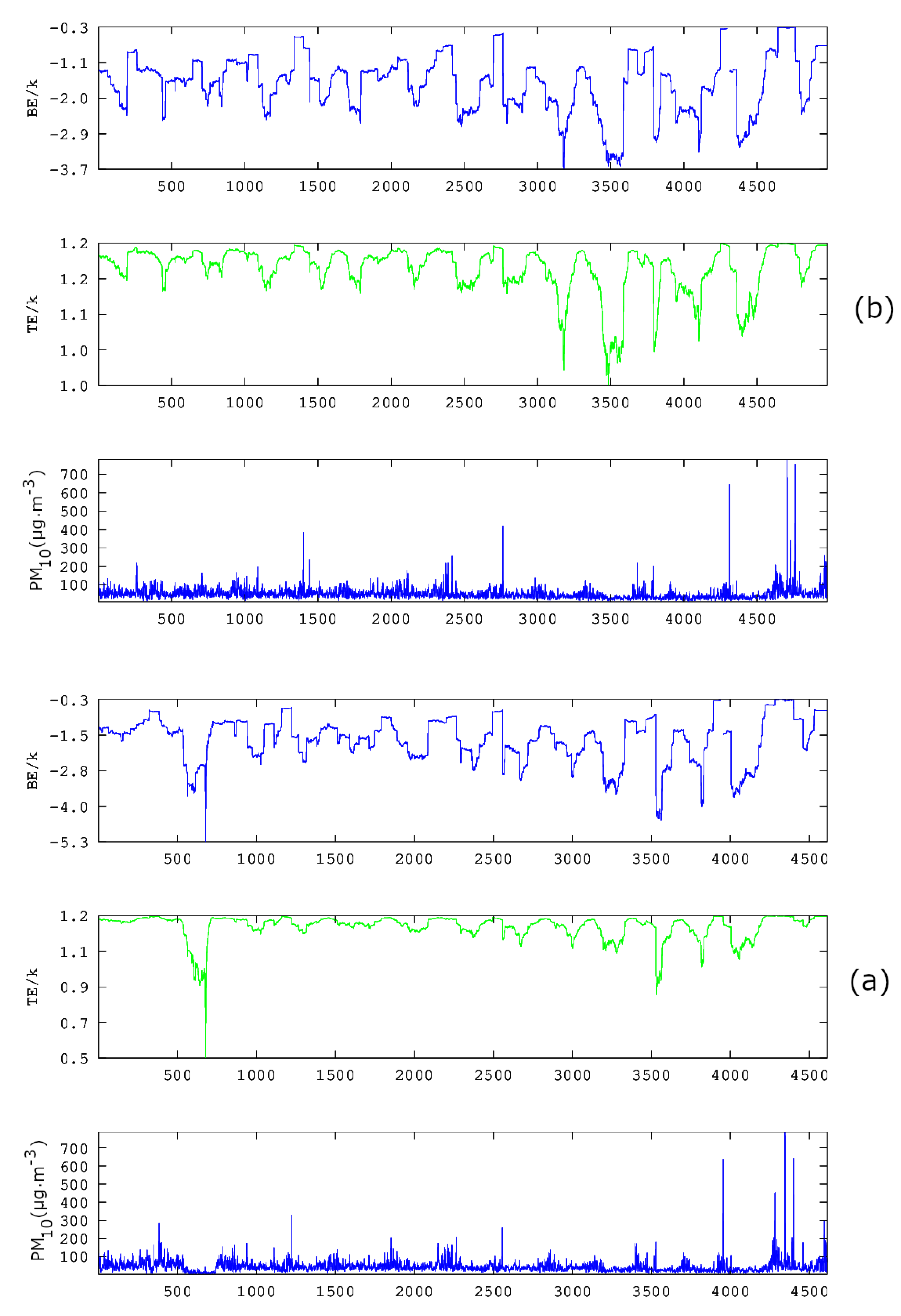
- In every time series window , the Boltzmann entropy is calculated aswhere k is the Boltzmann constant, i.e., . Boltzmann entropy is a measure of uncertainty and gives the average amount of information needed to predict the actual distribution of measurements in window i. Tsallis entropy is calculated aswhere k is the Boltzmann constant and q is a real number measuring the non-extensivity of the system [51]. k is taken as 1.8 according to previous publications [40,41].
3.5. Block Entropy Analysis
4. Results and Discussion
- combined, continuously altering, power-law fractal or SOC state interactions of the PM10 air pollution system with several diverse sources of pollutants such as industrial processes, vehicular emissions and energy production from power stations, coupled with complicated physical and chemical processes [27,34];
- non-linear dynamics governing the PM10 system defined by low-dimensional chaos [55]; and
- exogenous forces (e.g., meteorological processes and photochemical reactions) can amplify or reduce the linear and non-linear mechanisms of the interactions among the ambient pollutants, which can further complicate the temporal structure of the dynamics of ambient pollutant concentrations, leading to complex behaviour of the air pollution system [56].
5. Conclusions
- Statistical and entropy analysis methods are employed for the study of a 17-year PM10 time series recorded from five stations in Athens, Greece. The purpose is to investigate further the stochastic trends of the series and explore if non-stochastic periods of low entropy values exist.
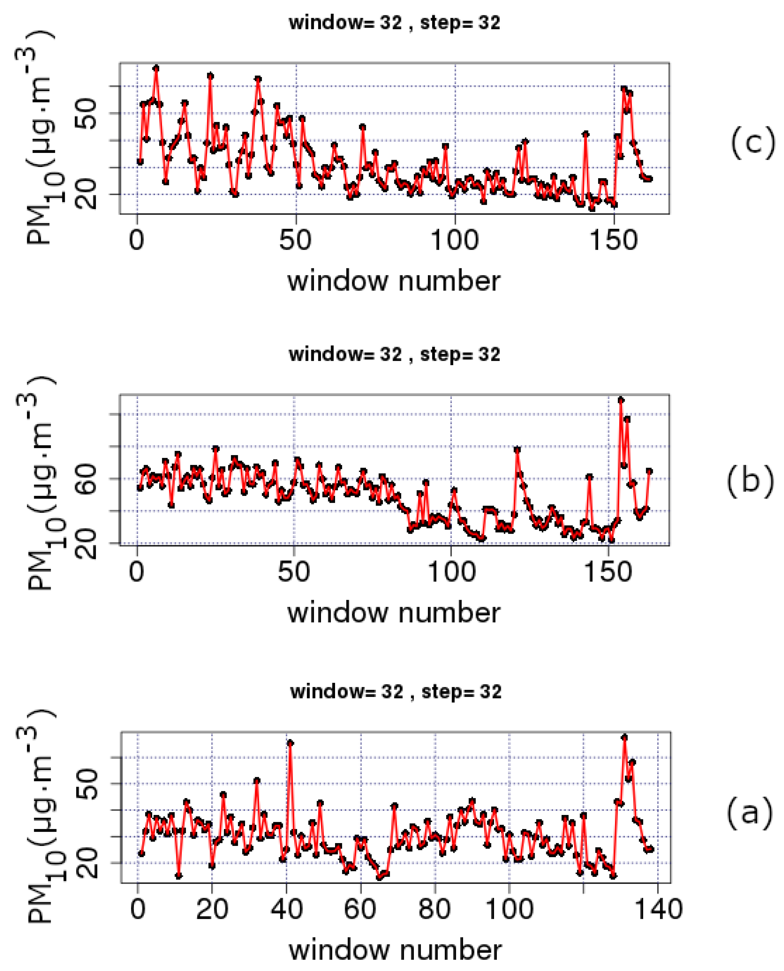
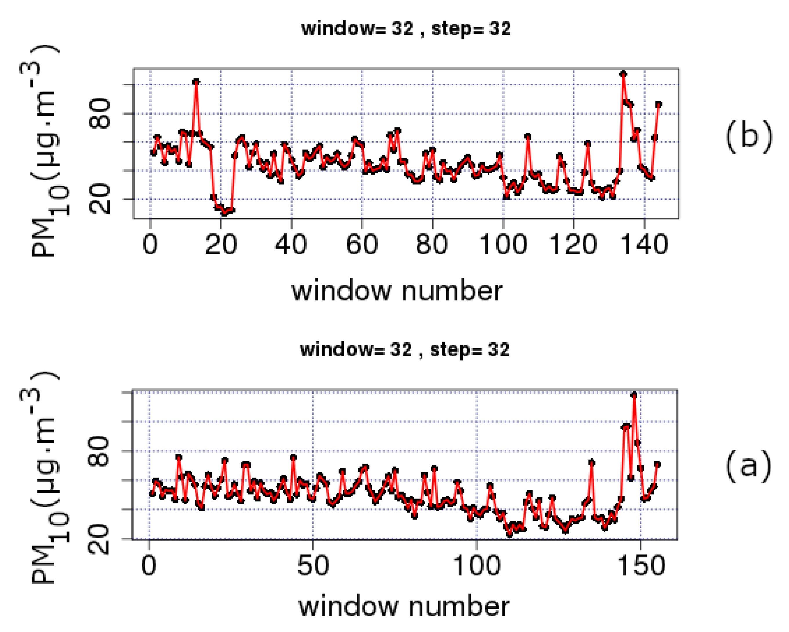
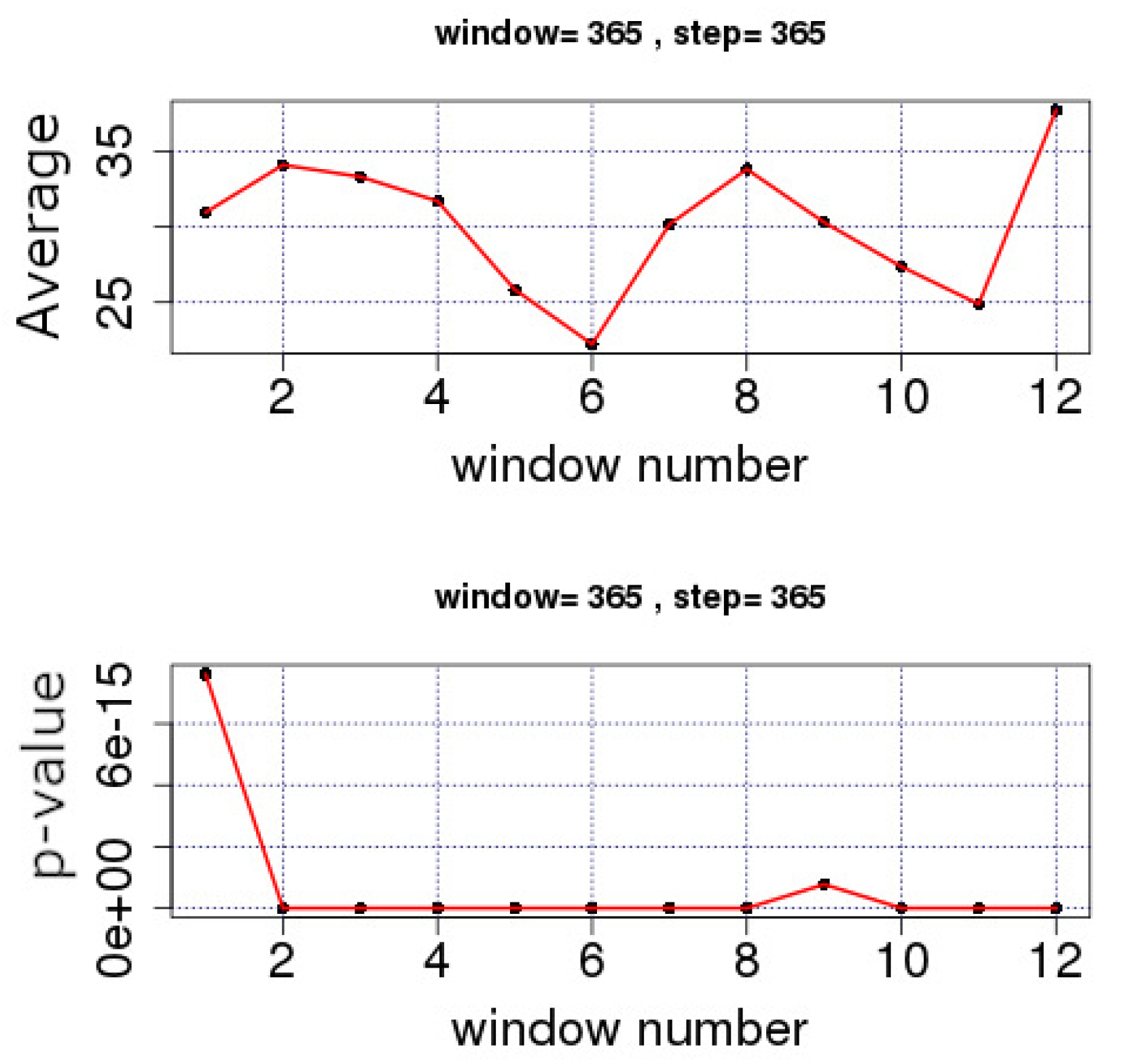
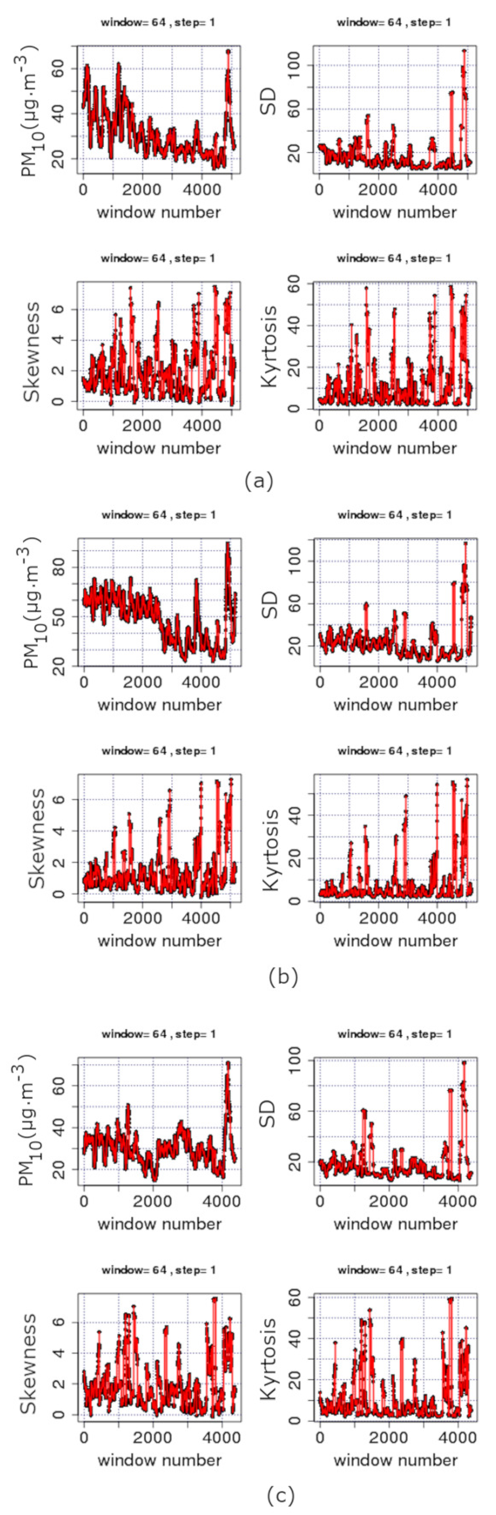
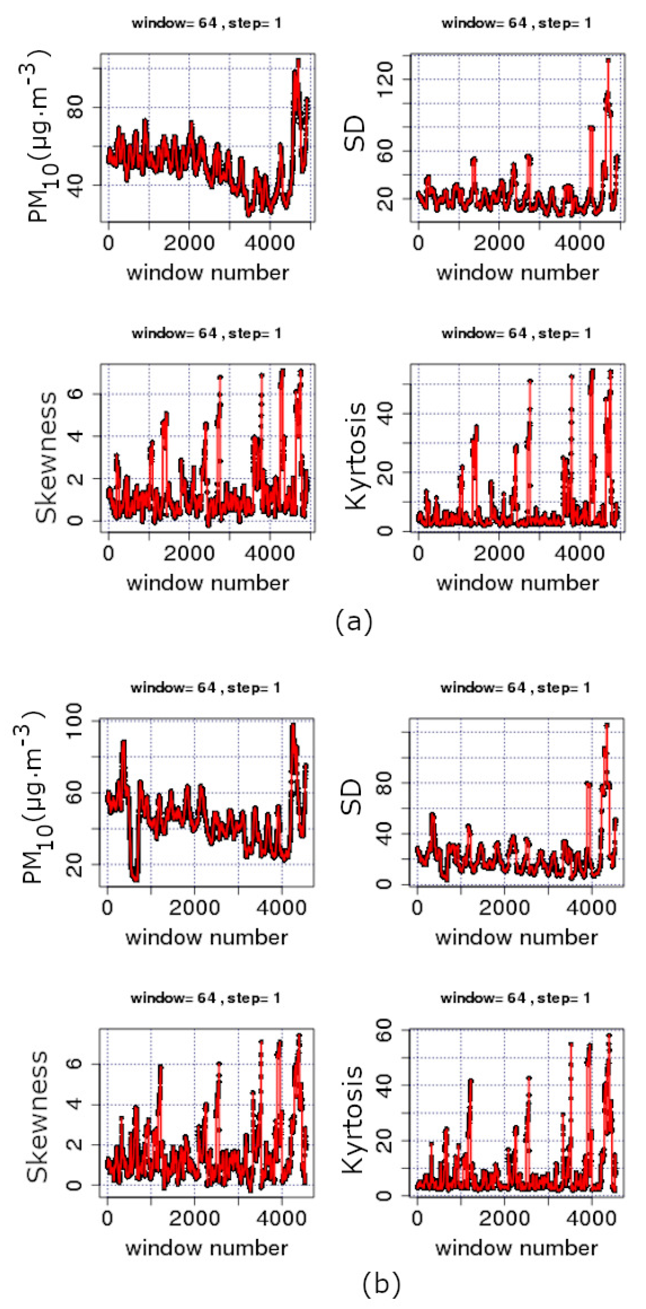
- The stochastic trends are analysed in monthly, two-month and annual windows via lumping and sliding windows. Decreasing time-evolution trends were found: (a) between Windows 40 and 130 for and a step of 32 (lumping process); and (b) between Windows 1 and 4000 for the AGP, THR, ARI and MAR series and between Windows 1 and 3500 for the LYK series, all for and a step of 1 (sliding window process). For Case (b), periods with high variance, skewness above 1 and kurtosis well above 3 are found. Deviations from the Gaussian distribution are addressed in various parts and, therefore, non-statistical behaviour. However, when the data are analysed for and a step of 365 (annual analysis through lumping), they follow the normal distribution. Several outliers are also found. ARI, LYK and MAR stations have similar IQR behaviour, indicating that LYK should be characterised as UT. The discrepancies from the stochastic behaviour are attributed to the multiple facets involved in physical procedures. The related mechanisms are discussed.
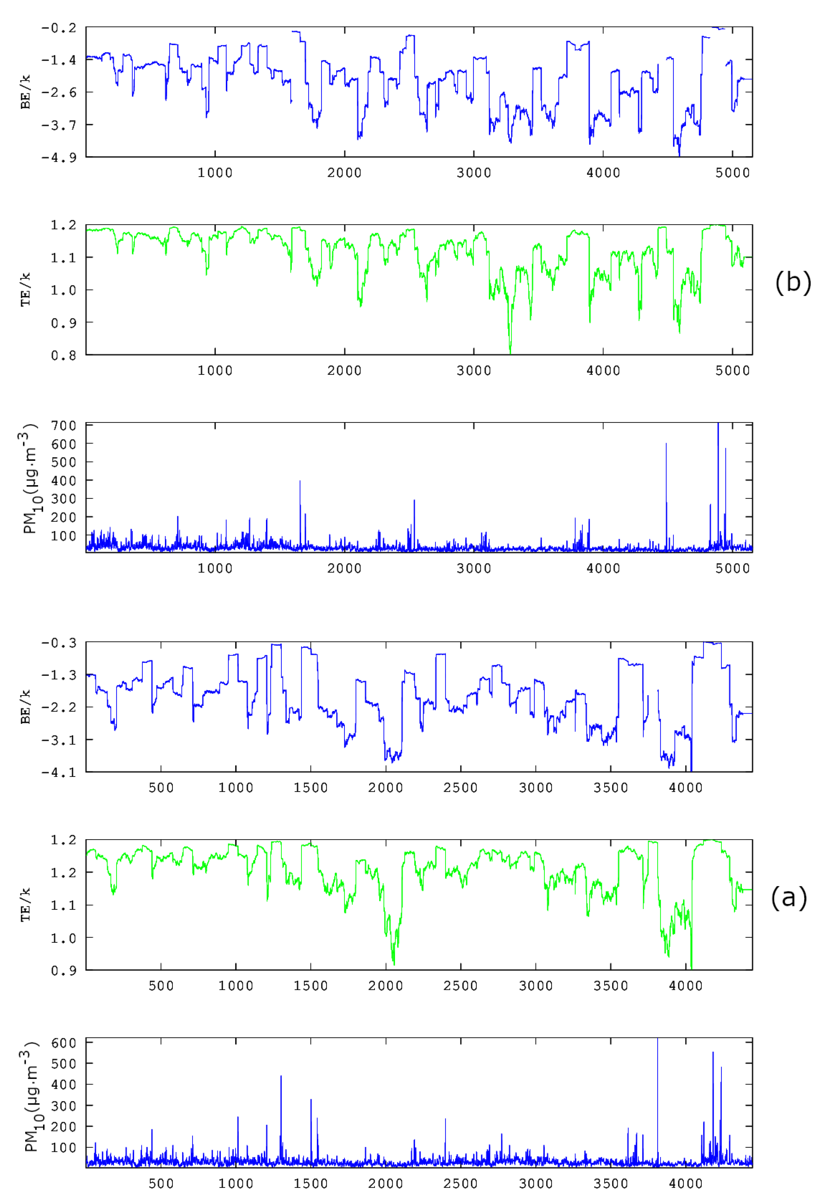
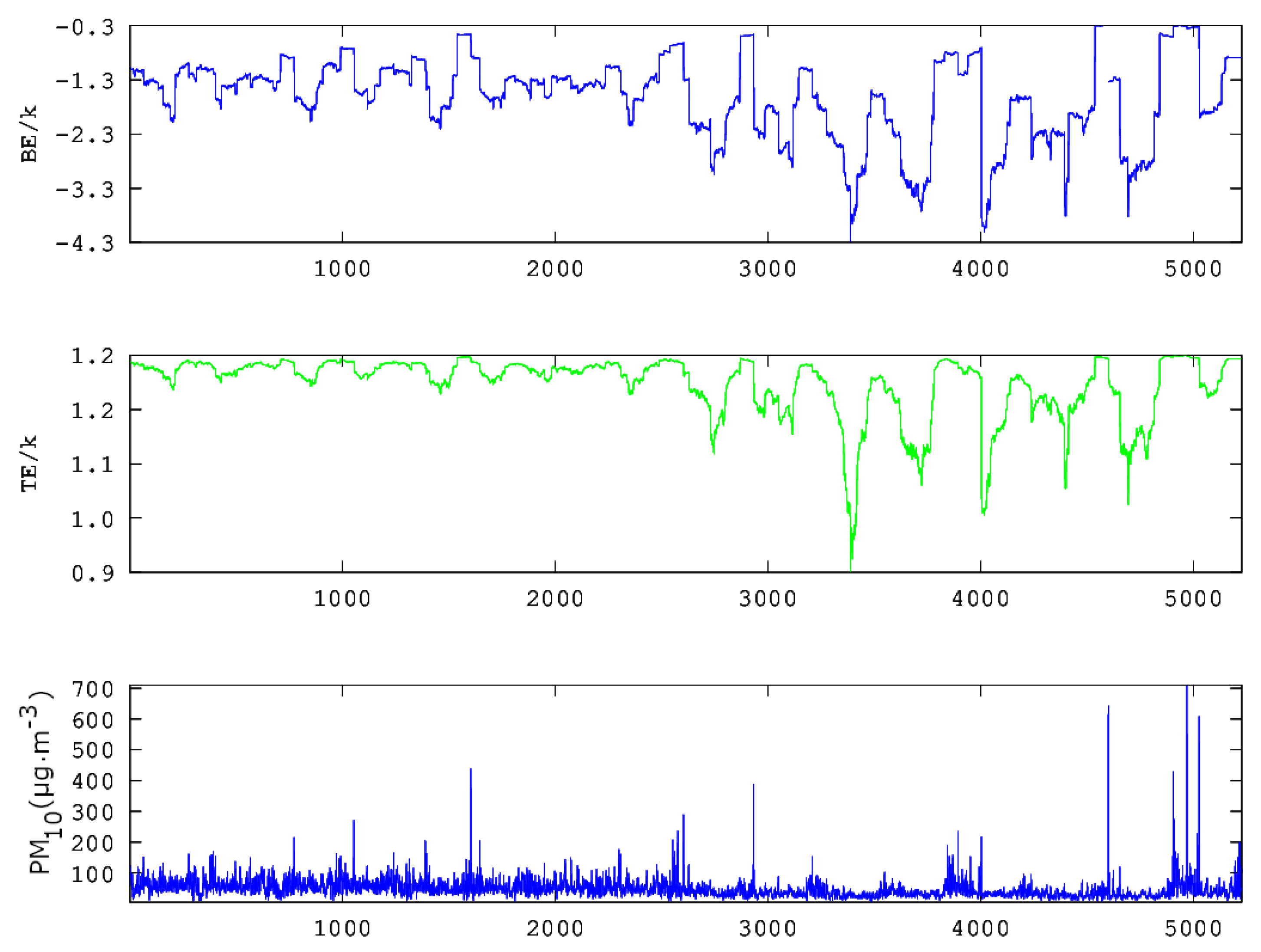
- Self organisation is investigated via Boltzmann and Tsallis entropy. Sliding windows of and a step of 1 are employed and symbolic dynamics in selected parts. The majority of the windows of all examined time series exhibit medium to low variations of both entropy values. Several low entropy parts are identified with Boltzmann entropy over Boltzmann constant below -2.0 entropy and Tsallis entropy over the Boltzmann constant below 1.18. The implications of the findings are discussed.
- A previously published combination two-step method is utilised to locate areas for which the PM10 system is out of stochastic behaviour and, simultaneously, exhibits critical self-organised patterns.According to previous publications, the non-stochastic periods are taken those with out of . These periods are located and extracted to ASCII data. The two-step methodology is applied to those periods and the critical entropy periods of Conclusion (b) above. Sixty-six different periods of two-month duration are found in the time series for various dates. From these, nine periods are common to at least three different stations. This is very significant because it is associated with internal dynamics of the GAA basin.
- Searching for enhanced evidence of SOC and fractal trends, as well as long memory, the findings of this study are further compared to previous publications for the same series. Two areas are found for which the series is non-stochastic and exhibit, simultaneously, fractal, long-memory and self-organisation patterns through a combination of 15 different fractal and SOC analysis techniques.
- In the two most significant areas, block entropy analysis is further applied. For comparison, block entropy is also utilised in the remaining identified parts with SOC patterns. Block entropy values are in the range 0.650–2.924 for words of 2–7 letters. Block entropy saturates above five letters. Significantly lower block entropy values are found for the two areas identified with the combination of 15 techniques, compared to the remaining areas.
- This is the first time to utilise entropy analysis for PM10 series and, importantly, in combination with results from previously published fractal methods. This combination approach is expected to be applied in the future to other environmental series, e.g., in environmental ozone and PM2.5 series, as well as in more seismic related series, such as radon in groundwater and soil and environmental electromagnetic disturbances. Despite the limited number of critical windows found, the enhanced evidence, on the one hand, and the increased outcomes, on the other hand, which are expected to be received in more dense time series, make the present approach a significant study tool. Future expectations are the extent of the methodology with multifractal techniques to account for the multifractality found in nature, as well as combining the present techniques with more advanced statistical approaches.
Author Contributions
Funding
Conflicts of Interest
References
- Chan, C.K.; Yao, X. Air pollution in mega cities in China. Atmos. Environ. 2008, 42, 1–42. [Google Scholar] [CrossRef]
- Fang, M.; Chan, C.K.; Yao, X.H. Managing air quality in a rapidly developing nation: China. Atmos. Environ. 2009, 43, 79–86. [Google Scholar] [CrossRef]
- Liu, Y.; Wang, T. Worsening urban ozone pollution in China from 2013 to 2017 – Part 1: The complex and varying roles of meteorology. Atmos. Chem. Phys. 2020, 20, 6305–6321. [Google Scholar] [CrossRef]
- Hand, J.L.; Prenni, A.; Copeland, S.; Schichtel, B.A.; Malm, W.C. Thirty years of the Clean Air Act Amendments: Impacts on haze in remote regions of the United States (1990–2018). Environment. Atmos. Environ. 2020, 243, 117865. [Google Scholar] [CrossRef]
- Thomas, D. Geochemical precursors to seismic activity. Pure Appl. Geophys. 1988, 126, 241–252. [Google Scholar] [CrossRef]
- Cíardenas Rodríguez, M.; Dupont-Courtade, L.; Oueslati, W. Air pollution and urban structure linkages: Evidence from European cities. Renew. Sust. Energ. Rev. 2016, 53, 1–9. [Google Scholar] [CrossRef]
- Lee, C. Impacts of urban form on air quality: Emissions on the road and concentrations in the US metropolitan areas. J. Environ. Manage. 2019, 246, 196–202. [Google Scholar] [CrossRef]
- Hinds, W.C. Aerosol Technology: Properties, Behavior, and Measurement of Airborne Particles, 2nd ed.; Wiley-VCH: Hoboken, NJ, USA, 1999; p. 53. [Google Scholar]
- Lee, Y.; Lee, J.; Kim, H.; Ha, E. Effects of PM10 on mortality in pure COPD and asthma-COPD overlap: Difference in exposure duration, gender, and smoking status. Sci. Rep. 2020, 10, 2402. [Google Scholar] [CrossRef] [Green Version]
- Hwang, J.; Bae, H.; Choi, S.; Yi, H.; Ko, B.; Kim, N. Impact of air pollution on breast cancer incidence and mortality: A nationwide analysis in South Korea. Sci. Rep. 2020, 5392, 770–808. [Google Scholar] [CrossRef]
- Zanobetti, A.; Schwartz, J. The effect of fine and coarse particulate air pollution on mortality: A national analysis. Health Perspect. 2009, 6, 898–903. [Google Scholar] [CrossRef] [Green Version]
- World Health Organisation. Air Quality Guidelines, 2nd ed.; WHO Regional Office for Europe: Copenhagen, Denmark, 2000; pp. 1–40. [Google Scholar]
- Lee, S.; Jang, M.; Oh, S.; Lee, J.; Suh, M.; Park, M. Associations between Particulate Matter and Otitis Media in Children: A Meta-Analysis. Int. J. Environ. Res. Public Health 2020, 17, 4604. [Google Scholar] [CrossRef] [PubMed]
- Zhang, F.; Luo, L.; Wang, Z.; Zhang, W.; Li, C.; Qiu, Z.; Huang, D. Estimation of the Effects of Air Pollution on Hospitalization Expenditures for Asthma. Int. J. Health Serv. 2020, 50, 100–109. [Google Scholar] [CrossRef]
- Tsoli, S.; Ploubidis, G.B.; Kalantzi, O.I. Particulate air pollution and birth weight: A systematic literature review. Atmos, Pollut. Res. 2019, 10, 1084–1122. [Google Scholar] [CrossRef]
- Braithwaite, I.; Zhang, S.; Kirkbride, J.; Osborn, D.; Hayes, J. Air Pollution (Particulate Matter) Exposure and Associations with Depression, Anxiety, Bipolar, Psychosis and Suicide Risk: A Systematic Review and Meta-Analysis. Environ. Health Perspect. 2019, 127, 12602. [Google Scholar] [CrossRef] [PubMed] [Green Version]
- Thompson, J.E. Airborne Particulate Matter. J. Occup. Environ. Med. 2018, 60, 392–423. [Google Scholar] [CrossRef] [PubMed]
- Nasser, Z.; Salameh, P.; Nasser, W.; Abou Abbas, L.; Elias, E.; Leveque, A. Outdoor particulate matter (PM) and associated cardiovascular diseases in the Middle East. Int. J. Occup. Med. Environ. Health 2015, 28, 641–661. [Google Scholar] [CrossRef]
- Goldberg, M. Particulate Air Pollution and Daily Mortality: Who Is at Risk? J. Aerosol. Med. 1996, 9, 43–53. [Google Scholar] [CrossRef]
- Ibarra-Berastegi, G.; Elias, A.; Barona, A.; Saenz, J.; Ezcurra, A.; de Argando na, J. From diagnosis to prognosis for forecasting air pollution using neural networks: Air pollution monitoring in Bilbao. Environ. Model. Softw. 2008, 23, 622–637. [Google Scholar] [CrossRef]
- Kourentzes, N.; Barrow, D.; Crone, S. Neural network ensemble operators for time series forecasting. Expert Syst. Appl. 2014, 41, 4235–4244. [Google Scholar] [CrossRef] [Green Version]
- Pérez, P.; Trier, A.; Reyes, J. Prediction of PM2.5 concentrations several hours in advance using neural networks in Santiago, Chile. Atmos. Environ. 2000, 34, 1189–1196. [Google Scholar] [CrossRef]
- Moustris, K.P.; Ziomas, I.C.; Paliatsos, A.G. 3-Day-Ahead Forecasting of Regional Pollution Index for the pollutants NO2, CO, SO2 and O3 using Artificial Neural Networks in Athens, Greece. Water Air Soil. Pollut. 2010, 224, 29–43. [Google Scholar] [CrossRef]
- Moustris, K.P.; Larisssi, I.K.; Nastos, P.T.; Koukouletsos, K.V.; Paliatsos, A.G. Development and Application of Artificial Neural Network Modeling in Forecasting PM10 Levels in a Mediterranean City. Water Air Soil Pollut. 2013, 224, 1–11. [Google Scholar] [CrossRef]
- Cacciola, M.; Pellicanó, D.; Megali, G.; Lay-Ekuakille, A.; Versaci, M.; Morabito, F.C. Aspects about Air Pollution prediction on urban environment. In Proceedings of the 4th Imeko TC19 Symposium on Environmental Instrumentation and Measurements Protecting Environment, Climate Changes and Pollution Control, Lecce, Italy, 3–4 June 2013; pp. 15–20. [Google Scholar]
- Catalano, M.; Galatioto, F.; Bell, M.; Namdeo, A.; Bergantino, A. Improving the prediction of air pollution peak episodes generated by urban transport networks. Environ. Sci. Policy 2016, 60, 69–83. [Google Scholar] [CrossRef] [Green Version]
- Kai, S.; Chun-qiong, L.; Nan-shan, A.; Xiao-hong, Z. Using three methods to investigate time-scaling properties in air pollution indexes time series. Nonlinear Anal. Real World Appl. 2008, 9, 693–707. [Google Scholar] [CrossRef]
- Liu, Z.; Wang, L.; Zhu, H. A time-scaling property of air pollution indices: A case study of Shanghai. China Atmos. Pollut. Res. 2015, 6, 886–892. [Google Scholar] [CrossRef]
- Varotsos, C.; Ondov, J.; Efstathiou, M. Scaling properties of air pollution in Athens, Greece and Baltimore. Md. Atmos. Environ. 2005, 39, 4041–4047. [Google Scholar] [CrossRef]
- Lee, C.K.; Juang, L.C.; Wang, C.C.; Liao, Y.Y.; Yu, C.C.; Liu, Y.C.; Ho, D.S. Scaling characteristics in ozone concentration time series (OCTS). Chemosphere 2006, 62, 934–946. [Google Scholar] [CrossRef] [PubMed]
- Windsor, H.L.; Toumi, R. Scaling and persistence of UK pollution. Atmos. Environ. 2001, 35, 4545–4556. [Google Scholar] [CrossRef]
- Weng, Y.C.; Chang, N.B.; Lee, T.Y. Nonlinear time series analysis of ground-level ozone dynamics in Southern Taiwan. J. Environ. Manag. 2008, 87, 405–414. [Google Scholar] [CrossRef]
- Xue, Y.; Pan, W.; Lu, W.z.; He, H.D. Multifractal nature of particulate matters (PMs) in Hong Kong urban air. Sci. Total Environ. 2015, 532, 744–751. [Google Scholar] [CrossRef]
- Dong, Q.; Wang, Y.; Li, P. Multifractal behavior of an air pollutant time series and the relevance to the predictability. Environ. Pollut 2017, 222, 444–457. [Google Scholar] [CrossRef]
- Broday, Y.D.M. Studying the time scale dependence of environmental variables predictability using fractal analysis. Environ. Sci. Technol. 2010, 44, 4629–4634. [Google Scholar] [CrossRef]
- Nikolopoulos, D.; Moustris, K.; Petraki, E.; Koulougliotis, D.; Cantzos, D. Fractal and Long-Memory Traces in PM10 Time Series in Athens, Greece. Environments 2019, 6, 29. [Google Scholar] [CrossRef] [Green Version]
- Nikolopoulos, D.; Moustris, K.; Petraki, E.; Cantzos, D. Long-memory traces in PM10 time series in Athens, Greece: Investigation through DFA and R/S analysis. Meteorol. Atmospheric Phys. 2020. [Google Scholar] [CrossRef]
- Nikolopoulos, D.; Petraki, E.; Yannakopoulos, P.; Priniotakis, G.; Voyiatzis, I.; Cantzos, D. Long-Lasting Patterns in 3 kHz Electromagnetic Time Series after the ML = 6.6 Earthquake of 2018-10-25 near Zakynthos, Greece. Geosciences 2020, 10, 235. [Google Scholar] [CrossRef]
- Alam, A.; Wang, N.; Zhao, G.; Mehmood, T.; Nikolopoulos, D. Long-lasting patterns of radon in groundwater at Panzhihua, China: Results from DFA, fractal dimensions and residual radon concentration. Geochem. J. 2019, 53, 341–358. [Google Scholar] [CrossRef]
- Petraki, E.; Nikolopoulos, D.; Fotopoulos, A.; Panagiotaras, D.; Nomicos, C.; Yannakopoulos, P.; Kottou, S.; Zisos, A.; Louizi, A.; Stonham, J. Long-range memory patterns in variations of environmental radon in soil. Anal. Methods 2013, 5, 4010–4020. [Google Scholar] [CrossRef]
- Nikolopoulos, D.; Petraki, E.; Vogiannis, E.; Chaldeos, Y.; Giannakopoulos, P.; Kottou, S.; Nomicos, C.; Stonham, J. Traces of self-organisation and long-range memory in variations of environmental radon in soil: Comparative results from monitoring in Lesvos Island and Ileia (Greece). J. Radioana.l Nucl. Chem. 2014, 299, 203–219. [Google Scholar] [CrossRef]
- Karamanos, K.; Nicolis, G. Symbolic Dynamics and Entropy Analysis of Feigenbaum Limit Sets. Chaos Soliton. Frac. 1999, 10, 1135–1150. [Google Scholar] [CrossRef]
- Moustris, K.; Petraki, E.; Ntourou, K.; Priniotakis, G.; Nikolopoulos, D. Spatiotemporal Evaluation of PM10 Concentrations within the Greater Athens Area, Greece. Trends, Variability and Analysis of a 19 Years Data Series. Environments 2020, 53, 85. [Google Scholar] [CrossRef]
- PM10 Full Dataset between 2001–2018 in Greece. Available online: https://ypen.gov.gr/perivallon/poiotita-tis-atmosfairas/dedomena-metriseon-atmosfairikis-rypansis/ (accessed on 1 February 2021).
- Authority, H.S. Population-Housing Census; Hellenic Statistical Authority: Piraeus, Greece, 2011. [Google Scholar]
- Climatic Data for Selected Stations in Greece. Available online: http://www.hnms.gr/emy/en/climatology/climatology_city?perifereia=Attiki&poli=Athens_Hellinikon/ (accessed on 1 February 2021).
- Amaral, S.; Carvalho, J.; Costa, M.; Pinheiro, C. An Overview of Particulate Matter Measurement Instruments. Atmosphere 2015, 6, 1327–1345. [Google Scholar] [CrossRef] [Green Version]
- Morales, I.O.; Landa, O.; Fossion, R.; Frank, A. Scale invariance, self-similarity and critical behaviour in classical and quantum system. J. Phys. Conf. Ser. 2012, 380, 12020. [Google Scholar] [CrossRef] [Green Version]
- Musa, M.; Ibrahim, K. Existence of long memory in ozone time series. Sains Malays. 2012, 41, 1367–1376. [Google Scholar]
- Petraki, E. Electromagnetic Radiation and Radon-222 Gas Emissions as Precursors of Seismic Activity. Ph.D. Thesis, Department of Electronic and Computer Engineering, Brunel University, London, UK, 2016. [Google Scholar]
- Kalimeri, M.; Papadimitriou, C.; Balasis, G.; Eftaxias, K. Dynamical complexity detection in pre-seismic emissions using non-additive Tsallis entropy. Physica A 2008, 387, 1161–1172. [Google Scholar] [CrossRef]
- Karamanos, K. Entropy analysis of substitutive sequences revisited. J Phys. A Math. Gen. 2001, 34, 9231–9241. [Google Scholar] [CrossRef]
- Izonin, I.; Tkachenko, R.; Verhun, V.; Zub, K. An approach towards missing data management using improved GRNN-SGTM ensemble method. Eng. Sci. Technol. Int. J. 2020. [Google Scholar] [CrossRef]
- Lu, W.; Xue, Y.; di He, H. Detrended fluctuation analysis of particle number concentrations on roadsides in Hong Kong. Build. Environ. 2014, 82, 580–S587. [Google Scholar] [CrossRef]
- Khokhlov, V.N.; Glushkov, A.V.; Loboda, N.S.; Bunyakova, Y.Y. Short-range forecast of atmospheric pollutants using non-linear prediction method. Atmos. Environ. 2008, 42, 7284–7292. [Google Scholar] [CrossRef]
- Yu, H.L.; Lin, Y.C.; Sivakumar, B.; Kuo, Y. A study of the temporal dynamics of ambient particulate matter using stochastic and chaotic techniques. Atmos. Environ. 2015, 69, 37–45. [Google Scholar] [CrossRef]


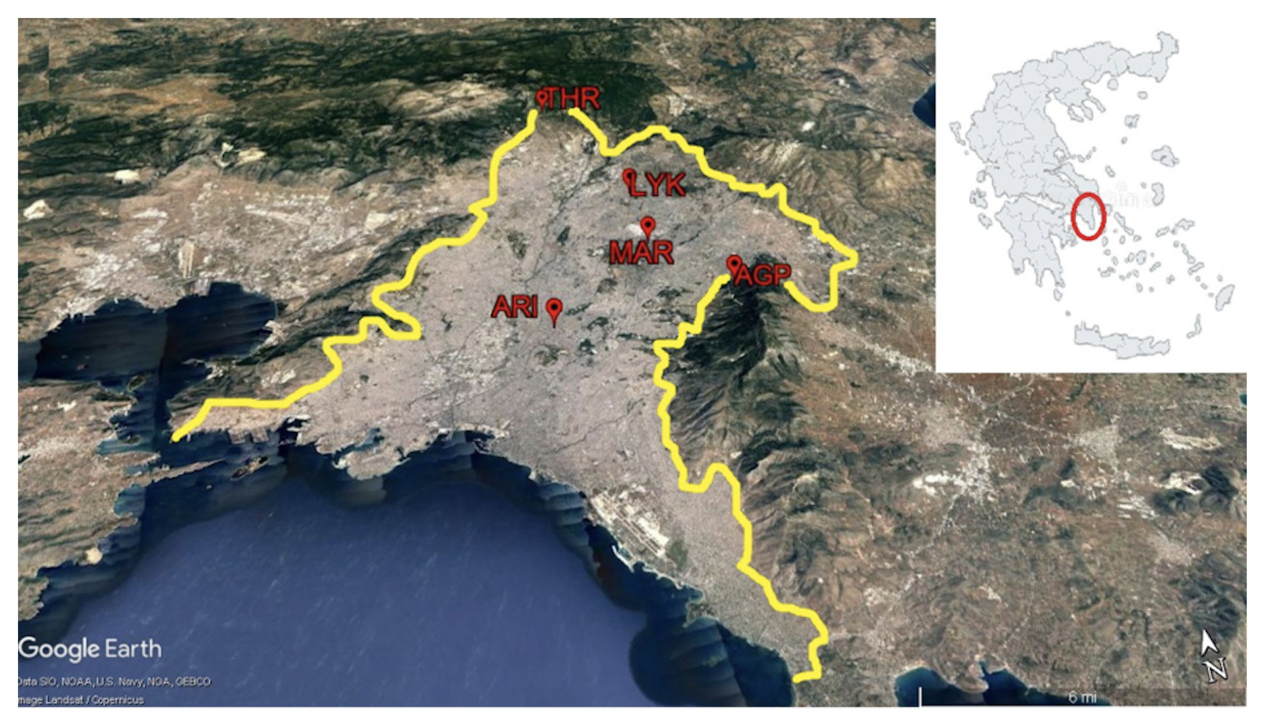
| Monitoring Station | Abbr. | Longitude | Latitude | Alt. (m) | Characterisation | D.C. |
|---|---|---|---|---|---|---|
| Aristotelous | ARI | 23°43’39" | 37°59’16" | 75 | Urban-Traffic | 85.8% |
| Lykovrissi | LYK | 23°47’19" | 38°04’04" | 234 | Suburban-Background | 89.2% |
| Maroussi | MAR | 23°47’14” | 38°01’51” | 170 | Urban-Traffic | 82.5% |
| Agia Paraskevi | AGP | 23°49’09” | 37°59’42” | 290 | Suburban-Background | 88.7% |
| Thrakomakedones | THR | 23°45’29’ | 38°08’36” | 550 | Suburban-Background | 77.2% |
| Monitoring Station | i/i | Date |
|---|---|---|
| AGP | 1 | 2005/12/3 |
| 2 | 2005/12/5 | |
| 3 | 2007/3/24 | |
| 4 | 2007/3/25 | |
| 5 | 2007/7/28 | |
| 5 | 2007/11/6 | |
| 6 | 2009/4/4 | |
| 7 | 2009/4/6 | |
| 7 | 2010/6/7 | |
| 8 | 2010/12/28 | |
| 9 | 2011/6/9 | |
| 10 | 2013/5/31 | |
| 11 | 2013/6/1 | |
| 12 | 2013/6/2 | |
| 13 | 2013/6/3 | |
| 14 | 2013/6/4 | |
| 15 | 2014/6/26 | |
| 16 | 2014/6/27 | |
| 17 | 2014/10/19 | |
| 17 | 2015/1/8 | |
| 18 | 2015/2/6 | |
| 19 | 2015/2/2 | |
| 20 | 2016/5/13 | |
| 20 | 2016/7/17 | |
| ARI | 1 | 2007/3/25 |
| 2 | 2009/4/4 | |
| 3 | 2009/4/6 | |
| 4 | 2010/3/5 | |
| 5 | 2010/3/6 | |
| 6 | 2010/3/7 | |
| 7 | 2010/3/8 | |
| 8 | 2014/6/26 | |
| 9 | 2014/6/27 | |
| 10 | 2015/2/6 | |
| 11 | 2015/2/2 | |
| 11 | 2016/5/13 | |
| 12 | 2016/7/17 | |
| LYK | 5 | 2007/7/28 |
| 1 | 2009/4/4 | |
| 2 | 2010/2/22 | |
| 3 | 2010/2/23 | |
| 4 | 2010/2/25 | |
| 5 | 2010/6/7 | |
| 6 | 2014/6/26 | |
| 7 | 2014/6/27 | |
| 8 | 2015/1/8 | |
| 9 | 2016/5/23 | |
| 10 | 2016/5/24 | |
| 11 | 2016/5/25 | |
| 12 | 2016/5/27 | |
| MAR | 1 | 2007/3/24 |
| 2 | 2007/3/25 | |
| 3 | 2007/6/14 | |
| 5 | 2007/7/28 | |
| 3 | 2009/4/4 | |
| 4 | 2009/4/6 | |
| 5 | 2010/2/22 | |
| 6 | 2010/2/23 | |
| 7 | 2010/6/7 | |
| 8 | 2014/6/26 | |
| 9 | 2014/6/27 | |
| 10 | 2015/1/8 | |
| 11 | 2015/1/22 | |
| 12 | 2015/2/6 | |
| 13 | 2015/2/2 | |
| 14 | 2015/2/7 | |
| 15 | 2016/7/22 | |
| THR | 1 | 2009/4/4 |
| 2 | 2009/4/6 | |
| 3 | 2010/12/28 | |
| 4 | 2011/6/9 | |
| 5 | 2015/2/6 | |
| 6 | 2015/2/2 | |
| 7 | 2016/7/17 |
| i/i | Date | Monitoring Stations |
|---|---|---|
| 1. | 2007/3/25 | AGP, ARI, MAR |
| 2007/7/28 | AGP, LYK, MAR | |
| 2. | 2009/4/4 | AGP, ARI, LYK, THR |
| 3. | 2009/4/6 | AGP, ARI, MAR, THR |
| 4. | 2010/6/7 | AGP, LYK, MAR |
| 5. | 2014/6/26 | AGP, ARI, LYK, MAR |
| 6. | 2014/6/27 | AGP, ARI, LYK, MAR |
| 2015/1/8 | AGP, LYK, MAR | |
| 7. | 2015/2/6 | AGP, ARI, MAR, THR |
| 8. | 2015/2/2 | AGP, MAR, THR |
| 9. | 2016/7/7 | AGP, ARI, THR |
| i/i | Date | Monitoring Stations | Techniques | Publication |
|---|---|---|---|---|
| 1. | 2007/7/28 | AGP, LYK, MAR | 13 different fractal techniques | Nikolopoulos et al. [36] |
| 2. | 2010/6/7 | AGP, LYK, MAR | 13 different fractal techniques | Nikolopoulos et al. [36] |
| 3. | 2015/1/8 | AGP, LYK, MAR | DFA & RS analysis | Nikolopoulos et al. [37] |
| Area 1 | Area 2 | Area Net | |||||
|---|---|---|---|---|---|---|---|
| Station | Letters | BE | TE | BE | TE | BE | TE |
| AGP | 2 | 1.095 | 0.682 | 1.108 | 0.650 | 1.231 | 0.743 |
| 3 | 1.679 | 0.896 | 1.143 | 0.699 | 1.847 | 0.921 | |
| 4 | 1.859 | 0.927 | 1.398 | 0.701 | 2.364 | 1.005 | |
| 5 | 2.095 | 0.997 | 1.834 | 0.939 | 2.847 | 1.064 | |
| 6 | 2.095 | 0.997 | 1.835 | 0.938 | 2.843 | 1.069 | |
| 7 | 2.097 | 0.996 | 1.832 | 0.943 | 2.846 | 1.062 | |
| ARI | 2 | 1.196 | 0.731 | 1.206 | 0.735 | 1.328 | 0.792 |
| 3 | 1.665 | 0.891 | 1.413 | 0.801 | 1.828 | 0.910 | |
| 4 | 2.119 | 1.009 | 1.678 | 0.900 | 2.442 | 1.039 | |
| 5 | 2.109 | 0.997 | 1.945 | 0.986 | 2.895 | 1.090 | |
| 6 | 2.111 | 0.998 | 1.946 | 0.987 | 2.897 | 1.091 | |
| 7 | 2.112 | 0.998 | 1.947 | 0.987 | 2.898 | 1.091 | |
| LYK | 2 | 1.045 | 0.651 | 1.305 | 0.789 | 1.267 | 0.757 |
| 3 | 1.708 | 0.892 | 1.751 | 0.907 | 1.887 | 0.936 | |
| 4 | 1.864 | 0.957 | 2.026 | 0.975 | 2.396 | 1.017 | |
| 5 | 1.981 | 0.976 | 2.138 | 1.015 | 2.924 | 1.094 | |
| 6 | 1.982 | 0.977 | 2.139 | 1.015 | 2.295 | 1.096 | |
| 7 | 1.981 | 0.978 | 2.141 | 1.016 | 2.297 | 1.097 | |
| MAR | 2 | 1.227 | 0.746 | 1.323 | 0.802 | 1.231 | 0.740 |
| 3 | 1.821 | 0.943 | 1.775 | 0.924 | 1.781 | 0.892 | |
| 4 | 2.211 | 1.024 | 2.211 | 1.024 | 2.281 | 0.986 | |
| 5 | 2.369 | 1.057 | 2.222 | 0.993 | 2.534 | 1.035 | |
| 6 | 2.371 | 1.059 | 2.221 | 0.995 | 2.532 | 1.037 | |
| 7 | 2.369 | 1.062 | 2.223 | 0.997 | 2.536 | 1.037 | |
| THR | 2 | 1.208 | 0.703 | 1.157 | 0.695 | 1.243 | 0.754 |
| 3 | 1.878 | 0.941 | 1.478 | 0.809 | 1.829 | 0.919 | |
| 4 | 1.841 | 0.946 | 1.925 | 0.974 | 2.397 | 1.031 | |
| 5 | 1.981 | 0.976 | 2.025 | 0.993 | 2.849 | 1.068 | |
| 6 | 1.983 | 0.977 | 2.027 | 0.991 | 2.856 | 1.069 | |
| 7 | 1.984 | 0.975 | 2.029 | 0.994 | 2.842 | 1.067 |
Publisher’s Note: MDPI stays neutral with regard to jurisdictional claims in published maps and institutional affiliations. |
© 2021 by the authors. Licensee MDPI, Basel, Switzerland. This article is an open access article distributed under the terms and conditions of the Creative Commons Attribution (CC BY) license (http://creativecommons.org/licenses/by/4.0/).
Share and Cite
Nikolopoulos, D.; Alam, A.; Petraki, E.; Papoutsidakis, M.; Yannakopoulos, P.; Moustris, K.P. Stochastic and Self-Organisation Patterns in a 17-Year PM10 Time Series in Athens, Greece. Entropy 2021, 23, 307. https://0-doi-org.brum.beds.ac.uk/10.3390/e23030307
Nikolopoulos D, Alam A, Petraki E, Papoutsidakis M, Yannakopoulos P, Moustris KP. Stochastic and Self-Organisation Patterns in a 17-Year PM10 Time Series in Athens, Greece. Entropy. 2021; 23(3):307. https://0-doi-org.brum.beds.ac.uk/10.3390/e23030307
Chicago/Turabian StyleNikolopoulos, Dimitrios, Aftab Alam, Ermioni Petraki, Michail Papoutsidakis, Panayiotis Yannakopoulos, and Konstantinos P. Moustris. 2021. "Stochastic and Self-Organisation Patterns in a 17-Year PM10 Time Series in Athens, Greece" Entropy 23, no. 3: 307. https://0-doi-org.brum.beds.ac.uk/10.3390/e23030307