
Stability of Non-Linear Dirichlet Problems with ϕ-Laplacian


Institute of Mathematics, Lodz University of Technology, Wólczańska 215, 90-924 Lodz, Poland
*
Author to whom correspondence should be addressed.
Entropy 2021, 23(6), 647; https://0-doi-org.brum.beds.ac.uk/10.3390/e23060647
Submission received: 5 May 2021
/
Revised: 19 May 2021
/
Accepted: 20 May 2021
/
Published: 22 May 2021
(This article belongs to the Special Issue Nonlinear Dynamics and Analysis)
Abstract
:We study the stability and the solvability of a family of problems with Dirichlet boundary conditions, where , u, are allowed to vary as well. Applications for boundary value problems involving the p-Laplacian operator are highlighted.
1. Introduction
The Hadamard Programme about non-linear equations concerns the following:
- (a)
- the solvability;
- (b)
- the uniqueness;
- (c)
- the dependence on parameters.
Note that (c) can be viewed (and is sometimes called) as a type of a stability, which is not to be confused with the Lyapunov stability as described in [1]. The issues named as (a) and (b) have been widely considered by the non-linear analysis methods (the variational method, the usage of critical point theory, the method of monotone operators, the degree theory, various fixed point results), see for example [2,3,4,5] to mention books covering the existence tools pertaining to the method of monotone operators applied here. Apart from the major reference books mentioned, there are a number of recent results dealing with the not necessarily variational existence of boundary value problems, and also with a type of approximation leading to the solvability of a given problem. Let us mention, without being exhaustive, for example, [6] where the celebrated Leray–Lions Theorem is utilized in order to generate a sequence which further approximates the solution to the Dirichlet problem with the -Laplacian. In [7], the Leray–Schauder degree is used to investigate the equations on integers governed by the -Laplacian which may further serve as an approximating sequence to some boundary value problem. Problems driven by the -Laplacian were investigated by the Harnack inequality, combined with fixed point approaches pertaining to the Bohnenblust–Karlin fixed point theorem in [8] and the Schauder, the Krasnosel’skii fixed point theorems in [9]. Boundary value problems for equations and systems with the p-Laplacian, as well as bounded or singular homeomorphisms are considered by the Krasnosel’skii type compression–expansion arguments and by a weak Harnack type inequality in [10].
On the other hand, the third issue has not been given that much attention, we can mention [11] describing the variational approach towards the dependence on parameters and also [12] where monotonicity methods are used. Some abstract scheme best reflecting the type of stability applied here allowing for various parameters is to be found in [13], where stability or well-posedness results are proved for families of semi-linear operator equations. There was also some research relating the dependence on eigenvalues of the Dirichlet problem with the p-Laplacian as p varies. All these sources mentioned employ the uniform bound on the sequence of solutions together with their weak characterization and suitable embedding results. There is also research in a different direction, which not only reflects the dependence on parameters. Namely, in [14] it is considered the convergence of eigenvalues of the p-Laplacian as by using approximation of functions by functions in the sense of strict convergence on . Paper [15] concerns the case of the variational eigenvalues of the -Laplacian under the uniform convergence of the exponents investigated by variational methods. We mention also the recent [16] which treats problems with the right hand side independent of the sought function which investigates the dependence of gradients of solutions as . In this paper, we are concerned with the dependence on non-linear functional parameters for problems governed by the p-Laplacian also with p being treated as a numerical parameter. Contrary to [11,12,13] we do not concentrate only on problems governed by the (negative) Laplacian but include the boundary problems driven by p-laplacian for into our consideration. Moreover, the approach towards the stability is based not on the investigation of the sequence of solutions corresponding to the sequence of parameters but on the analysis of the solution operators which makes our main stability result, namely Theorem 4, independent of the existence method (among mentioned above) which is employed in order to prove the solvability of the relevant (non-linear) equation. We allow for due to tools which we apply for the solvability. An easy example best illustrating what sort of problems we may encounter now follows.
Example 1.
Let us consider for the following family of Dirichlet problems with and :
Note that for every there exists a solution to (1). If we let and then it is direct to observe that (1) is unsolvable with , , see [17] for details. This observation we supply with the following additional conclusions: is not bounded in which means that it is not weakly convergent up to a subsequence, hence it is not (weakly) compact in .
In what follows we will provide some general conditions which exclude the phenomena appearing above, as well as conditions on under which one obtains the convergence in Example 1. The paper is organized as follows. We start with some preliminaries about functional space setting, illustrating the relations between spaces involved by some figure and providing some version of the well known Krasnosel’skii Theorem on the continuity of the Niemytskij operator, as well as some general stability results. Boundary value problems with the -Laplacian are next considered with the right hand side independent of the sought function and for which the existence and stability result. The existence is reached by a direct formula exploiting the properties of the increasing homeomorphism and the stability is obtained by investigating the continuity of the solution operator. Next, with the aid of the Browder–Minty Theorem such results are shifted to problems containing non-linear perturbations. Examples and comments are included into the text, corresponding also to the Dirac delta thus showing the possible general applicability of our results.
2. Preliminaries and Auxiliary Results
Following [17] we denote by , , the space of all absolutely continuous functions with -integrable derivative. For another approach towards the Sobolev spaces on , see [18]. We refer is the sequel to both sources for the background. If not said otherwise, we consider any . We endow with a standard norm
Recall that inclusion is continuous for every p and compact if . We denote
and consider it with a norm
equivalent with on . A continuous dual of will be denoted by , here and in the sequel q is the Hölder conjugate to p, that is . We put and denote a continuous dual of by . The Poincaré and the Sobolev inequalities are as follows: for all we have
where and is the optimal constant in the Poincaré inequality. Ref. [19] [Chapter 1, Section 4] contains detailed calculations of this constant. The mapping is increasing and continuous on and . Notice that as an immediate consequence of the Sobolev inequality we obtain
where stands for a norm in . Denote by j an continuous embedding given by
Functional is called regular if for some . We denote
Identifying via the Riesz’ Representation Theorem we get . Moreover, a mapping defined by
is an isometry between and . Hence is an isometry between (identified with a dual of ) and . Notice that for all and that
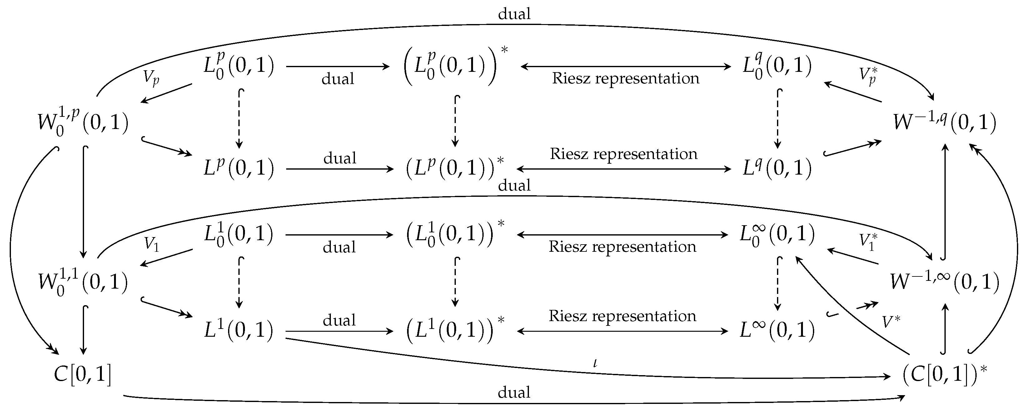
for every regular f and any p. Moreover, continuous inclusion provides that for every p. Therefore, we can define a continuous linear operator using a formula , which coincides with the Formula (3) for every regular f. Let us observe that compact inclusion , , provides that in . Here denotes a weak* convergence of sequence to element . From now on we equip with a weak* topology. These relations are summarized in Figure 1.
Now we turn to the Niemytskii operator. For a closed set denote
Let be a Carthéodory function, that is:
- is Lebesgue-measurable for all ;
- is continuous for a.e. .
The following result is a direct consequence of the Lebesgue Dominated Convergence Theorem.
Theorem 1.
Assume that , and , all in . If there exists a function such that
then in .
Proof.
Without lost of generality we can assume that , and pointwisely a.e. on . Therefore, assumed continuity of provides
Finally, the assumption (4) allows us to apply the Lebesgue Dominated Convergence Theorem. □
Let us consider a compact metric space and a Banach space X. Let be a continuous mapping such that for every bounded set , the set is relatively compact in X. We denote
Lemma 1.
Assume that A satisfies conditions given above and let in Σ. Then every sequence such that for , either has a subsequence convergent to some or else it holds satisfy .
Proof.
Define . The continuity of A tells us that S is closed. Let . Since , it follows that sets are compact for all . Hence, whenever and , every bounded subsequence of has a further subsequence such that . The continuity of A allows us to conclude that . □
The results obtained can be expressed in terms of the upper semi-continuity of multi-valued mappings, see [20]. However we do not need such a general approach here.
Now, let us consider a real, reflexive and separable Banach space X. Operator is called coercive if
T is monotone if
and T is strongly continuous if in X implies that in . We say that T is bounded if is bounded in for every bounded .
Theorem 2
([21]). Assume that is continuous, coercive, and bounded. If additionally , where is monotone and is strongly continuous, then .
3. Boundary Value Problems with the -Laplacian
We denote by the space of all homeomorphism of the real line, equipped with a topology of almost uniform convergence, namely, we write if and only if for every compact . Direct calculations provide that whenever . We will consider with a distance , where . Thus it makes sense to write with no confusion. For a fixed and fixed we consider
Solutions to (5) are understood in the following sense: an absolutely continuous function is a solution to (5) if , if is integrable and if
Notice that approach introduced covers also classical cases where the right hand side of (5) is continuous or integrable.
Example 2.
The assumption about allows us to consider problems of the form
where , and is the Diracs delta, that is
Now we follow with a stability result which best reflects how we understand the dependence on parameters.
Theorem 3.
Let in and in . Then problem (5) (with and ) has a unique solution for each . Moreover, in for every p.
For the proof of Theorem 3 we need an auxiliary lemma, which describes properties of the solution operator. Note that we can replace with , equipped with a weak topology, using the continuous embedding and retain all the assertions.
Lemma 2.
For each and for every , there exists a unique satisfying
Moreover, for every bounded sets and every norm-bounded set , a mapping is bounded and continuous.
Proof.
For all and we define by (7). Function is continuous, strictly monotone and . Hence for a unique . Notice that for every increasing we have
since and since . Hence, the boundedness of c on follows from inequalities
which hold for every . Now, let in K and in . Then up to a subsequence (not renumbered). Moreover, in and the sequence is a.e. uniformly bounded. Hence we can use Theorem 1 to get in for every p. Then
and hence . This proves the continuity of c. □
Since for all , using Lemma 2 we obtain a classical solution to (5):
Therefore, in our setting, notions of weak and classical solution overlap. Now we are in the position to proceed with the proof of main result.
Proof of Theorem 3
Remark 1.
If functionals are regular, that is for , then assuming in , we get in . One can deduce it easily from (8) bearing in mind that in such a case
4. Non-Linear Perturbations of the -Laplcian Problems
Take a closed set . We consider the following assumption.
Theorem 4.
Proof.
Take any and denote by an operator mapping pairs into a unique weak solution to (5), which is given by (8). Define the Nemytskii operator associated with g by
The continuity and boundedness of follows form the assumption (10) and Theorem 1. Using the continuity of inclusion we obtain that the mapping
is also continuous and bounded on bounded sets. Define a mapping given by
Since sequences , , and are convergent, and since mappings and are continuous, is also continuous. Moreover for every bounded set , the boundedness of sequences and provides that set is bounded in and, hence, a relatively weak compact. Theorem 3 provides the continuity of on S and, hence, the relative compactness of . Therefore, we can use Lemma 1 with , and to get the assertion. □
Existence and Dependence on Parameters
For we denote the essential range of u by
and consider the following assumption. The advantage of using the essential range follows from the Example 3.
Theorem 5.
Proof.
For every we define the operators by
Using both, the Sobolev and the Poincaré inequalities together with assumption (13) we get
for all , which implies coercivity of . Moreover, we see that -norm of any solution to (14) is bounded by term . The monotonicity of and can be checked following (15) and [22], while the strongly continuity of is a consequence of Theorem 1 and compact inclusions , . Therefore, we can use the Browder–Minty Theorem to get the existence of a solution to (14) for every . Notice that an additional assumption about the convergence of and provides that . Hence we get and, therefore, we can use Theorem 4 to obtain required convergence . Finally, notice that the monotonicity of implies that
This clearly implies the uniqueness of a solution and finishes the proof. □
Example 3.
Let and in , , and in and in . Assume that
has a solution for every . Taking and we can apply Theorem 4 to obtain whenever , , , and in , where
Allowing for we do not meet the problems encountered in Example 1.
5. Discussion
This research provides additional advanced and complex information concerning the Hadamard Programme about non-linear equations. Our input relies on the fact that apart to standard parameter dependence we also allow for some structure stability with respect to the differential operator which is allowed to vary as far as it is still an increasing homeomorphism. The state of the art pieces concerned either the sole dependence on functional parameters (also incorporating some information whether the solution is of variational type which is not that important if one knows that this is a solution) or else these were concerned on the asymptotic analysis of the operator with reference to its eigenvalues. Our approach was to somehow coin the two approaches and allow the functional parameter to vary together with the differential operator. The second advance with reference to the dependence on parameters is that now we allow for quite a general type of parameters, i.e., the Dirac delta where the information can somehow be packed in one particle and, thus, leading a way to applications in physics. In the sources mentioned in the bibliography and also in those which cite them, the parameters are assumed rather regular. The methods pertain to the fixed point and monotone ones indicating that a possible further impact is also possible if one tries, with a modified approach, to use operators with more general monotonicity than the increasing homeomorphism.
Author Contributions
Conceptualization, M.B., M.G., I.K.; methodology, M.B., M.G., I.K.; software, M.B. and I.K.; validation, M.B., M.G., I.K.; formal analysis, M.G.; investigation, M.B., M.G., I.K.; writing—original draft preparation, M.B. and I.K.; writing—review and editing, M.B., M.G., I.K.; visualization, M.B. and I.K.; supervision, M.G.; project administration, M.G.; funding acquisition, M.G. and I.K. All authors have read and agreed to the published version of the manuscript.
Funding
This research received no external funding.
Data Availability Statement
Not applicable.
Acknowledgments
This paper has been completed while one of the authors—Michał Bełdziński, was the Doctoral Candidate in the Interdisciplinary Doctoral School at the Lodz University of Technology, Poland.
Conflicts of Interest
The authors declare no conflict of interest.
Abbreviations
The following abbreviations are used in this manuscript:
| MDPI | Multidisciplinary Digital Publishing Institute |
| DOAJ | Directory of open access journals |
| TLA | Three letter acronym |
| LD | Linear dichroism |
References
- Perko, L. Differential Equations and Dynamical Systems; Springer: New York, NY, USA, 2001. [Google Scholar]
- Dinca, G.; Jebelean, P.; Mawhin, J. No Title Variational and topological methods for Dirichlet problems with p-Laplacian. Port. Math. Nova Sér. 2001, 58, 339–378. [Google Scholar]
- Fučík, S.; Kufner, A. Studies in Applied Mathematics, 2: Nonlinear Differential Equations; Elsevier Scientific Publishing Company: Amsterdam, The Netherlands; Oxford, UK; New York, NY, USA, 1980. [Google Scholar]
- Motreanu, D.; Radulescu, V.D. Variational and Non-Variational Methods in Nonlinear Analysis and Boundary Value Problems; Springer US: New York, NY, USA, 2003. [Google Scholar]
- Papageorgiou, N.S.; Rǎdulescu, V.D.; Repovš, D.D. Nonlinear Analysis—Theory and Methods; Springer: Cham, Switzerland, 2019. [Google Scholar]
- Avci, M. Solutions to p(x)-Laplace type equations via nonvariational techniques. Opusc. Math. 2018, 38, 291–305. [Google Scholar] [CrossRef]
- Avci, M. A topological result for a class of anisotropic difference equations. Ann. Univ. Craiova Math. Comput. Sci. Ser. 2019, 46, 328–343. [Google Scholar]
- Precup, R.; Rodríguez-López, J. Positive solutions for discontinuous problems with applications to ϕ-Laplacian equations. J. Fixed Point Theory Appl. 2018, 20, 1–17. [Google Scholar] [CrossRef]
- Chinní, A.; Di Bella, B.; Jebelean, P.; Precup, R. A four-point boundary value problem with singular ϕ-Laplacian. J. Fixed Point Theory Appl. 2019, 21, 66. [Google Scholar] [CrossRef]
- Herlea, D.R.; Precup, R. Existence, localization and multiplicity of positive solutions to ϕ-laplace equations and systems. Taiwan. J. Math. 2016, 20, 77–89. [Google Scholar] [CrossRef]
- Ledzewicz, U.; Schättler, H.; Walczak, S. Optimal control systems governed by second-order ODEs with Dirichlet boundary data and variable parameters. Ill. J. Math. 2003, 47, 1189–1206. [Google Scholar] [CrossRef]
- Galewski, M. On the application of monotonicity methods to the boundary value problems on the Sierpinski gasket. Numer. Funct. Anal. Optim. 2019, 40, 1344–1354. [Google Scholar] [CrossRef]
- Idczak, D. Stability in semilinear problems. J. Differ. Equ. 2000, 162, 64–90. [Google Scholar] [CrossRef] [Green Version]
- Littig, S.; Schuricht, F. Convergence of the eigenvalues of the p-Laplace operator as p goes to 1. Calc. Var. Partial. Differ. Equ. 2014, 49, 707–727. [Google Scholar] [CrossRef]
- Colasuonno, F.; Squassina, M. Stability of eigenvalues for variable exponent problems. Nonlinear Anal. Theory Methods Appl. 2015, 123, 56–67. [Google Scholar] [CrossRef] [Green Version]
- Buccheri, S.; Leonori, T.; Rossi, J.D. Strong convergence of the gradients for p-Laplacian problems as p→∞. J. Math. Anal. Appl. 2021, 495, 124724. [Google Scholar] [CrossRef]
- Mawhin, J. Problemes de Dirichlet Variationnels Non Linéaires; Presses de l’Université de Montréal: Montréal, QC, Canada, 1987; Volume 1. [Google Scholar]
- Brezis, H. Functional Analysis, Sobolev Spaces and Partial Differential Equations; Springer Science & Business Media: Berlin/Heidelberg, Germany, 2010. [Google Scholar]
- Drábek, P.; Krejčí, P.; Takáč, P. Nonlinear Differential Equations; Chapman & Hall/CRC: Boca Raton, FL, USA, 1999. [Google Scholar]
- Hu, S.; Papageorgiou, N.S. Handbook of Multivalued Analysis. Volume I: Theory; Kluwer Academic Publishers: Dordrecht, The Netherlands, 1997. [Google Scholar]
- Franců, J. Monotone operators. A survey directed to applications to differential equations. Appl. Math. 1990, 35, 257–301. [Google Scholar] [CrossRef]
- Galewski, M. Basic Monotonicity Methods with Some Applications; To appear in Compact Textbooks in Mathematics; Birkhäuser: Basel, Switzerland; SpringerNature: Basingstoke, UK, 2021; ISBN 978-3-030-75308-5. [Google Scholar]
Figure 1.
Dashed ↪ denotes an inclusion, ↪—continuous and dense inclusion, —a compact and dense inclusion.
Figure 1.
Dashed ↪ denotes an inclusion, ↪—continuous and dense inclusion, —a compact and dense inclusion.

Publisher’s Note: MDPI stays neutral with regard to jurisdictional claims in published maps and institutional affiliations. |
© 2021 by the authors. Licensee MDPI, Basel, Switzerland. This article is an open access article distributed under the terms and conditions of the Creative Commons Attribution (CC BY) license (https://creativecommons.org/licenses/by/4.0/).
Share and Cite
MDPI and ACS Style
Bełdziński, M.; Galewski, M.; Kossowski, I. Stability of Non-Linear Dirichlet Problems with ϕ-Laplacian. Entropy 2021, 23, 647. https://0-doi-org.brum.beds.ac.uk/10.3390/e23060647
AMA Style
Bełdziński M, Galewski M, Kossowski I. Stability of Non-Linear Dirichlet Problems with ϕ-Laplacian. Entropy. 2021; 23(6):647. https://0-doi-org.brum.beds.ac.uk/10.3390/e23060647
Chicago/Turabian StyleBełdziński, Michał, Marek Galewski, and Igor Kossowski. 2021. "Stability of Non-Linear Dirichlet Problems with ϕ-Laplacian" Entropy 23, no. 6: 647. https://0-doi-org.brum.beds.ac.uk/10.3390/e23060647
Note that from the first issue of 2016, this journal uses article numbers instead of page numbers. See further details here.