
Why Dilated Convolutional Neural Networks: A Proof of Their Optimality


Department of Computer Science, University of Texas at El Paso, El Paso, TX 79968, USA
*
Author to whom correspondence should be addressed.
Entropy 2021, 23(6), 767; https://0-doi-org.brum.beds.ac.uk/10.3390/e23060767
Submission received: 18 April 2021
/
Revised: 14 June 2021
/
Accepted: 14 June 2021
/
Published: 18 June 2021
(This article belongs to the Special Issue Fractal and Multifractal Analysis of Complex Networks)
Abstract
:One of the most effective image processing techniques is the use of convolutional neural networks that use convolutional layers. In each such layer, the value of the layer’s output signal at each point is a combination of the layer’s input signals corresponding to several neighboring points. To improve the accuracy, researchers have developed a version of this technique, in which only data from some of the neighboring points is processed. It turns out that the most efficient case—called dilated convolution—is when we select the neighboring points whose differences in both coordinates are divisible by some constant ℓ. In this paper, we explain this empirical efficiency by proving that for all reasonable optimality criteria, dilated convolution is indeed better than possible alternatives.
1. Introduction
1.1. Convolutional Layers: Input and Outpu
At present, one of the most efficient techniques in image processing and in other areas is a convolutional neural network; see, e.g., [1]. Convolutional neural networks include special types of layers that perform linear transformations.
Each such layer is characterized by integer-values parameters , , , and ; then:
- the input to this layer consists of the values , where , , and are integers for which , , and ; and
- the output of this layer consists of the values , where d, x, and y are integers for which , , and .
1.2. Convolutional Layer: Transformation
A general linear transformation has the form
for some coefficients .
Transformations performed by a convolutional layer are a specific case of such generic linear transformations, where the following two restrictions are imposed:
- first, each value depends only on the values , for which both differences and do not exceed some fixed integer L, and
- the coefficients depend only on the differences and :for some coefficients defined for all pairs for which .
The values are known as a filter.
The resulting linear transformation takes the form
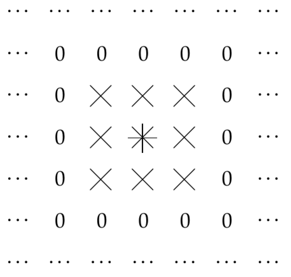
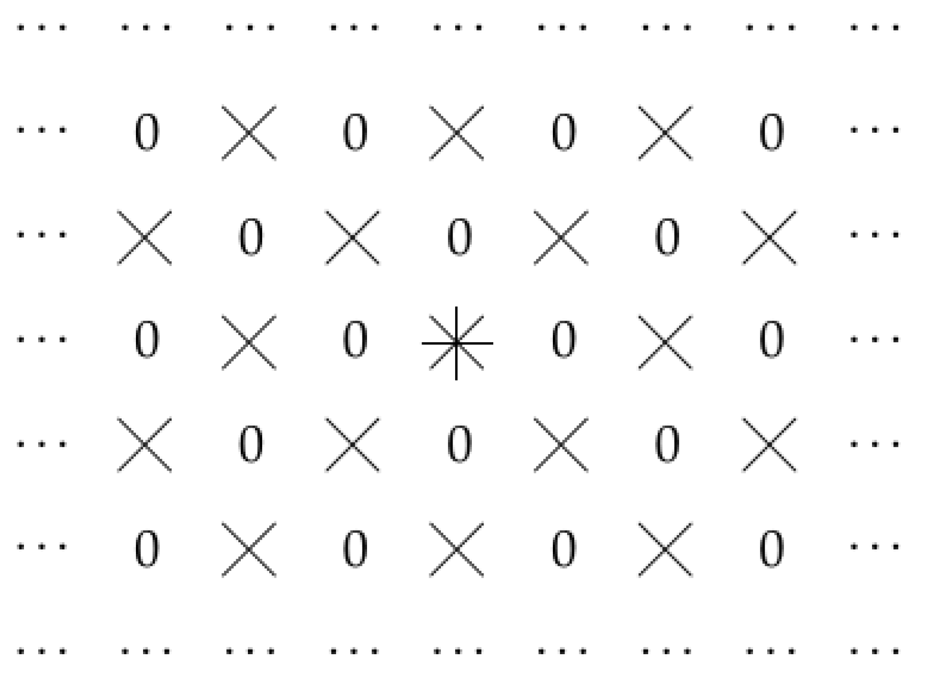
Thus, the output of a convolutional layer corresponding to the point is determined by the values of the input to this layer at points corresponding to and . This is illustrated by Figure 1, where, for and for a point marked by an asterisk, we show all the points that determine the values . For convenience, points that do not affect the values , are marked by zeros.
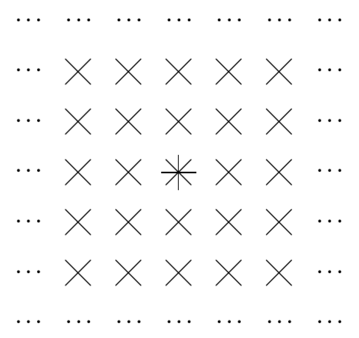
For , a similar picture has the following form. This is illustrated by Figure 2.
1.3. Sparse Filters and Dilated Convolution
Originally, convolutional neural networks used filters in which all the values for can be non-zero. It turned out, however, that we can achieve a better accuracy if we consider sparse filters, i.e., filters in which, for some pairs with , all the values are fixed at 0; see, e.g., [2,3,4].
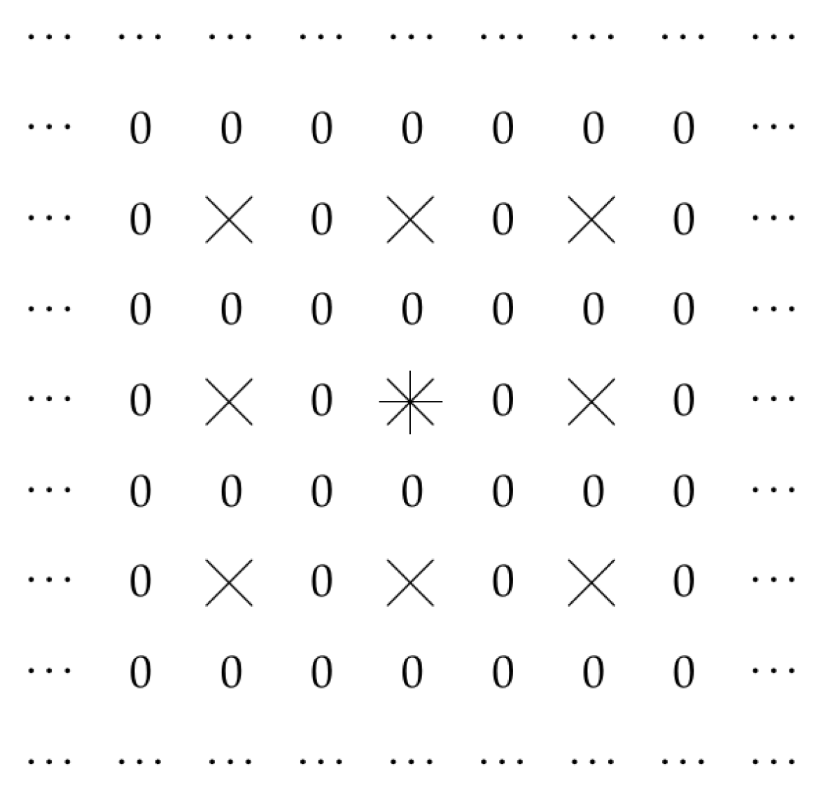
In Figure 3, we show an example of such a situation, when and only values , for which both i and j are even allowed to be non-zero.
In general, it turned out that such a restriction works best if we only allow for pairs which are divisible by some integer ℓ, i.e., if we take
In this case, the layer’s output signal can be written in the following equivalent form:
where we denoted , , , and .
1.4. Empirical Fact That Needs Explanation
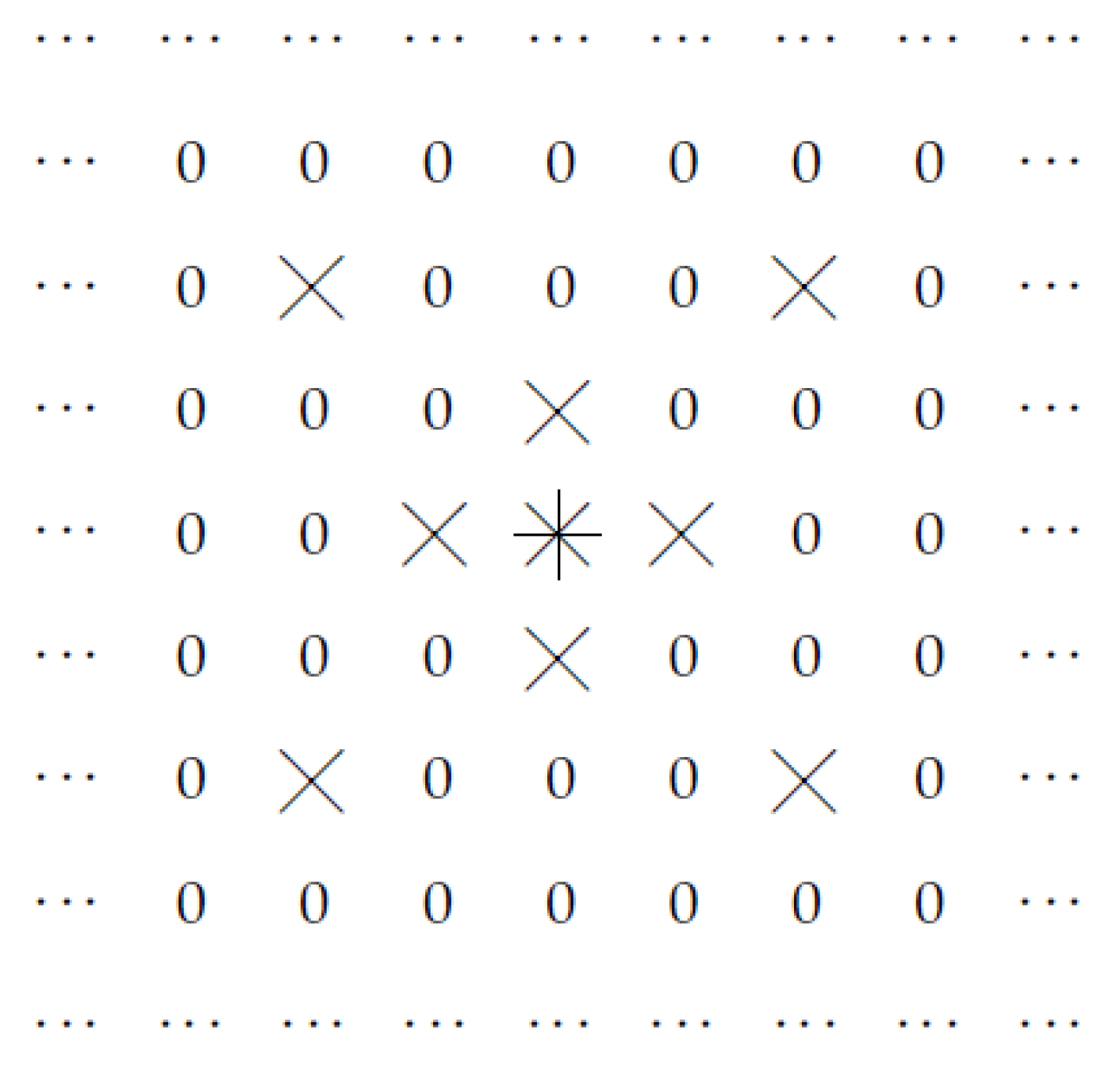
In principle, we could select other points at which the filter can be non-zero. For example, we could select points for which j is even, but i can be any integer. This is illustrated by Figure 4.
Alternatively, for , as points at which can be non-zero, we could select the points , , , and , see Figure 5.
However, empirical evidence shows that the selection corresponding to dilated convolution—when we select points for which i and j are both divisible by some integer ℓ—works the best [2,3,4].
To the best of our knowledge, there is no theoretical explanation for this empirical result—that dilated convolution leads to better results that select other sets of non-zero-valued points . The main objective of this paper is to provide such an explanation.
Comment. Let us emphasize that the only objective of this paper is to explain this empirical fact; we are not yet at a stage where we can propose a new method or even any improvements to the known methods.
2. Analysis of The Problem
2.1. Let Us Reformulate This Situation in Geometric Terms: Case of Traditional Convolution
In the original convolution Formula (1), to find the values , the layer’s output signal at a point , we need to know the values , the layer’s input signal at all the points of the type for . We can reformulate it by saying that we need to know the values at all the points at which the distance
does not exceed L:
where we denoted
We use, in this formula, the bounded subset D of the “grid” and not the whole set only matters at the border of the domain D. So, to simplify our formulas, we can follow the usual tradition (see, e.g., [3]) and simply use the whole set instead of the bounded set D:
Comment. Note that the set is potentially infinite. What makes the set of all the points —which affects the values —finite is the restriction , whose meaning is that such points should belong to the corresponding neighborhood of the point .
2.2. Case of Dilated Convolution
The dilated convolution can be described in a similar way. Namely, we can describe the Formula (4) as
where denotes the set of all the points for which both differences and are divisible by ℓ:
Note that, in this representation of dilated convolution, while we have several different sets for different points , there is only one filter , namely the same filter that was used in the original representation (4). So, in this new representation, we have exactly as many parameters as before.
The main difference between this formula and the Formula (9) is that, in contrast to the usual convolution (9), where the same set could be used for all the points , here, in general, we may need different sets for different points .
For example, if , then we need four such sets:
In this case, instead of the single set (as in the case of the traditional convolution), we have a set of such sets
To avoid confusion, we will call subsets of the original “grid” sets, while the set of such sets will be called a family. In these terms, the Formula (10) can be described as follows:
where denotes the set from the family that contains the point :
In this representation, all four sets S from the family are infinite—just like the set corresponding to the traditional convolution is infinite. Similarly to the traditional convolution, what makes the set of all the points —which affects the values —finite is the restriction , whose meaning is that such points should belong to the corresponding neighborhood of the point .
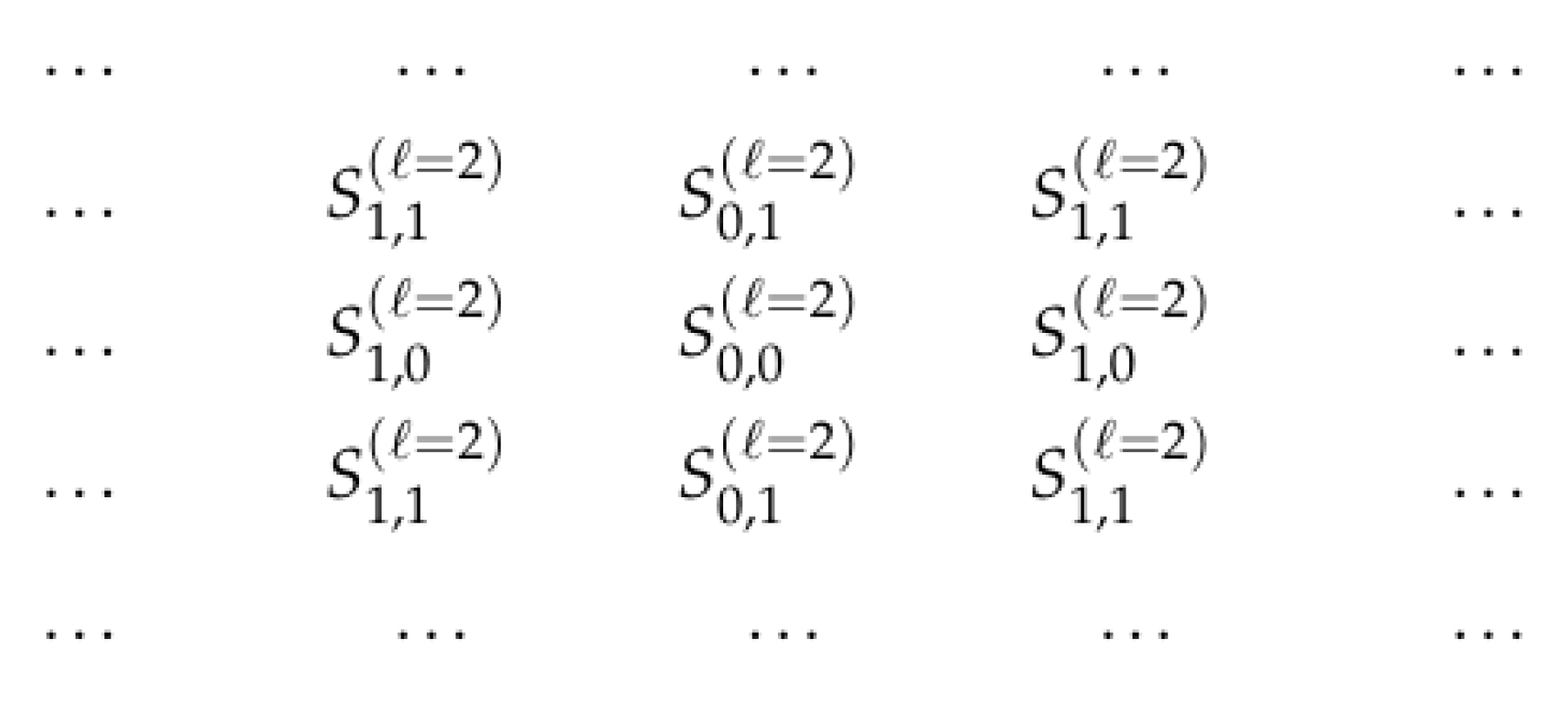
Figure 6 describes which of the four sets corresponds to each point from the “grid” :
For , we can get a similar reformulation, with the family
where is the set of all the pairs , in which both differences and are divisible by 3.
In general, for an arbitrary point , we should use the set
2.3. Other Cases
Such a representation is possible not only for dilated convolution. For example, the above case when we allow arbitrary value i and require the value j to be even can be described in a similar way, with
where:
- for points for which y is even, we take
- and for points for which y is odd, we take
We can also have families which have an infinite number of sets; an example of such a family will be given below.
We can also, in principle, consider the situations when we do not require that the coefficients depend only on the differences and . Thus, we arrive at the following general description.
2.4. General Case
In the general case, we get the following situation:
- we have a family of subsets of the “grid” ;
- the values of the layer’s output signal at a point are determined by the formulafor some values , where denotes the set from the family that contains the point .
For the Formula (23) to uniquely determine the values , we need to make sure that the set is uniquely determined by the point , i.e., that for each point , the family contains one, and only one, set S that contains this point. In other words:
- different sets from the family must be disjoint, and
- the union of all the sets must coincide with the whole “grid” .
In mathematical terms, the family must form a partition of the “grid” .
Comment. To avoid possible confusion, it is worth mentioning that while different sets S from the family are disjoint, this does not preclude the possibility that sets and corresponding to different points can be identical. For example, in the description of the traditional convolution, the family consists of only one set . In this case, for all points and , we have .
In terms of sets corresponding to different points, disjointness means that if the sets and are different, then these sets must be disjoint: .
2.5. We Do Not a Priori Require Shift-Invariance
Please note that we do not a priori require that the sets and corresponding to two different points and should be obtained from each other by shift—this property is known as shift invariance and is satisfied both for the usual convolution and for the dilated convolution.
It should be emphasized, however, that we will show that this shift-invariance property holds for the optimal arrangement.
2.6. Let Us Avoid the Degenerate Case
From a purely mathematical viewpoint, we can have a partition of the “grid” into one-point sets . This is an example when the family has infinitely many subsets.
In this case, no matter what value L we choose, the Formula (23) implies that the values of the layer’s output signal at a point are determined only by the values of the layer’s input at this same point. This is equivalent to using a convolution with ; such a convolution is known as the 1-by-1 convolution.
While such a convolution is often useful, in this case, for each point , there is only one point , so it is not possible to select only some of the points —which is the whole idea of dilation. Since, in this paper, we study dilation, we will therefore avoid this 1-by-1 situation and additionally require that at least one set from the family should contain more than one element.
2.7. What We Plan to Do
We will consider all possible families that form a partition of the “grid” , and we will show that for all optimality criteria that satisfy some reasonable conditions, the optimal family is either the family of sets corresponding to the dilated convolution—or a natural modification of this family.
Let us describe what we mean by optimality criteria.
2.8. What Does “Optimal” Mean?
In our case, we select between different families of sets , , …. In general, we select between alternatives a, b, etc. Out of all possible alternatives, we want to select an optimal one. What does “optimal” mean?
In many cases, “optimal” is easy to describe:
- we have an objective function that assigns a numerical value to each alternative a—e.g., the average approximation error of the numerical method a for solving a system of differential equations, and
- optimal means that we select an alternative for which the value of this objective function is the smallest possible (or, for some objective functions, the largest possible).
However, this is not the only possible way to describe optimality.
For example, if we are minimizing the average approximation error, and there are several different numerical methods with the exact same smallest value of average approximation error, then we can use this non-uniqueness to select, e.g., the method with the shortest average computation time. In this case, we have, in effect, a more complex preference relation between alternatives than in the case when decision is made based solely on the value of the objective function. Specifically, in this case, an alternative b is better than the alternative a—we will denote it by —if:
- either we have ,
- or we have and .
If this still leaves several alternatives which are equally good, then we can optimize something else, and thus, have an even more complex optimality criterion.
In general, having an optimality criterion means that we are able to compare pairs of alternatives—at least some such pairs—and conclude that:
- for some of these pairs, we have ,
- for some of these pairs, we have , and
- for some others pairs, we conclude that alternatives a and b are, from our viewpoint, of equal value; we will denote this by .
Of course, these relations must satisfy some reasonable properties. For example, if b is better than a, and c is better than b, then c should be better than a; in mathematical terms, the relation < must be transitive.
We must have some alternative which is better than or equivalent to all others—otherwise, the optimization problem has no solutions. It also makes sense to require that there is only one such optimal alternative—indeed, as we have mentioned, if there are several equally good optimal alternatives, this means that the original optimality criterion is not final, that we can use this non-uniqueness to optimize something else, i.e., in effect, to modify the original criterion into a final (or at least “more final”) one.
2.9. Invariance
There is an additional natural requirement for possible optimality criteria, which is related to the fact that the original “grid” has lots of symmetries, i.e., transformations that transform this “grid” into itself.
For example, if we change the starting point of the coordinate system to a new point , then a point that originally had coordinates now has coordinates . It makes sense to require that the relative quality of two different families and will not change if we simply change the starting point.
Similarly, we can change the direction of the x-axis, then a point becomes . If we change the direction of the y-axis, we obtain a transformation . Finally, we can rename the coordinates: what was x will become y and vice versa; this corresponds to the transformation . Such transformations should also not affect the relative quality of different families.
Please note that we are not requiring that the family of sets be shift-invariant, what we require is that the optimality criterion is shift-invariant.
Let us explain why, in our opinion, it makes sense to require that the optimality criterion is shift-invariance—as well as having other invariance properties. Indeed, let us consider any usual optimality criterion such as accuracy of classification, robustness to noise, etc. What each criterion means is, e.g., the overall classification accuracy over the set of all possible cat and not-a-cat images . We want this method to correctly classify images into cats and not-cats, whether these images are centered or somewhat shifted. Thus, to adequately compare different methods, we should test these methods on a set of images that includes both original and shifted images.
Here:
- if we shift each image I from the set by the same shift , i.e., replace each image by a shifted image for which ,
- then, we should get, in effect, the exact same set of images:
The only difference between these two sets of images may be the few images where the cat is right at the image’s boundary; in this paper, we will ignore this difference—just like we ignored the bounded-ness in the previous text. In this ignoring-bounds approximation, we conclude that
How does a shift of the original image affect the input signals to the following convolution layers? In between the very first input layer and the following convolution layers, we may have (and usually do have) layers that perform the “compression” of the part—i.e., that transform:
- values corresponding to several points
- into values corresponding to a single new point .
In general, the -shift of the original data corresponds to a shift of the transformed data—but by smaller shift values. For example, if data corresponding to each new -point come from data from four different “pre-compression” points, then the shift by in the pre--compression layer corresponds to a shift of the convolution layer input by .
Since the set of input images should not change if we apply a shift, we can conclude that for each convolution layer, the set of the corresponding inputs to this layer should also not change if we shift all these inputs, i.e., if we replace each input with a shifted input
for some shift .
The set of inputs on which we compare different methods does not change when we apply a shift. So, if one method was better when we processed original inputs, it should still be better if we process shifted inputs—since the resulting set of inputs is the same. In other words, the quality (e.g., accuracy) of a method corresponding to the family , when gauged by the set of inputs corresponding to original images, should be the same as this method’s quality on the set
of all the inputs obtained from the original set by this shift—since these two sets of inputs are, in effect, the same set: . Thus, .
However, as one can see, shifting all the inputs is equivalent to shifting all the sets from the family . Indeed, if we apply the Formula (23) to the shifted layer’s input , we get
i.e., in terms of the shifted coordinates and for which and , we get—taking into account that the distance does not change with shift—that:
where we denoted
and where denotes the condition .
In terms of the family , the main difference between the Formulas (23) and (29) is that instead of the condition , we now have a new condition
i.e., equivalently, . It is easy to check that this new condition is equivalent to , where the new family is obtained by shifting sets from the original family .
So:
- the relative quality of two families does not change if we shift all the layer’s inputs;
- however, shifting all the layer’s inputs is equivalent to shifting all the sets from the family .
Thus, the relative quality of two families does not change if we shift both families. In other words, a reasonable optimality criterion—which describes which family is better—should be invariant with respect to shifts.
Similarly, we can argue that a reasonable optimality criterion should not change if we rename x- and y-axes, etc.
Now, we are ready for the precise formulation of the problem.
3. Definitions and the Main Result
Definition 1.
By a family, we mean a family of non-empty subsets of the “grid” , a family in which:
- all sets from this family are disjoint, and
- at least one set from this family has more than one element.
Terminological comment. To avoid possible misunderstandings, let us emphasize that here, we consider several levels of sets, and to avoid confusion, we use different terms for sets from different levels:
- first, we consider points ;
- second, we consider sets of points ; we call them simply sets;
- third, we consider sets of sets of points ; we call them families;
- finally, we consider the set of all possible families ; we call this a class.
Comment about the requirements. In the previous text, we argued that for each family , the union of all its sets should coincide with the whole “grid” . However, in our definition of an alternative, we did not impose this requirement. We omitted this requirement to make our result stronger—since, as we see from the following Proposition, this requirement actually follows from all the other requirements.
Definition 2.
By an optimality criterion, we mean a pair of relations on the class of all possible families that satisfy the following conditions:
- if and , then ;
- if and , then ;
- if and , then ;
- if and , then ;
- we have for all ; and
- if , then we cannot have .
Comment. The pair of relations between families of subsets forms what is called a pre-order or quasi-order. This notion is more general than partial order, since, in contrast to the definition of the partial order, we do not require that if and , then : in principle, we can have for some .
Definition 3.
We say that a family is optimal with respect to the optimality criterion , if for every other family , we have either or .
Definition 4.
We say that the optimality criterion is final if there exists exactly one family which is optimal with respect to this criterion.
Definition 5.
By a transformation , we mean one of the following transformations: , , , and .
Definition 6.
For each family and for each transformation T, by the result of applying the transformation T to the family , we mean the family , where, for any set S,
Definition 7.
We say that the optimality criterion is invariant if for all transformations T, implies that , and implies that .
Proposition 1.
For every final invariant optimality criterion, the optimal family is equal, for some integer , to one of the following two families:
- the family of all the sets corresponding to all possible pairs of integers for which ;
- the family of all the setscorresponding to all possible pairs of integers for which .
Comments.
- This proposition takes care of all invariant (and final) optimality criteria. Thus, it should work for all usual criteria based on misclassification rate, time of calculation, used memory, or any others used in neural networks: indeed, if one method is better than another for images in general, it should remain to be better if we simply shift all the images or turn all the images upside down. Images can come as they are, they can come upside down, they can come shifted, etc. If, for some averaging criterion, one method works better for all possible images, but another method works better for all upside-down versions of these images—which is, in effect, the same class of possible images—then, from the common sense viewpoint, this would mean that something is not right with this criterion.
- The first possibly optimal case corresponds to dilated convolution. In the second possibly optimal case, the optimal family contains similar but somewhat different sets; an example of such a set is given in Figure 7.Thus, this result explains the effectiveness of dilated convolution—and also provides us with a new alternative worth trying.
Proof.
. Since the optimality criterion is final, there exists exactly one optimal family . Let us first prove that this family is itself invariant, i.e., that for all transformations T.
Indeed, the fact that the family is optimal means that for every family , we have or . Since this is true for every family , it is also true for every family , where denotes inverse transformation (i.e., a transformation for which ). Thus, for every family , we have either or . Due to invariance, we have or . By definition of optimality, this means that the alternative is also optimal. However, since the optimality criterion is final, there exists exactly one optimal family, so .
The statement is proven.
. Let us now prove that the optimal family contains a set that, in its turn, contains the point and some point
Indeed, by definition of a family, every family—including the optimal family—contains at least one set S that has at least two points. Let S be any such set from the optimal family, and let be any of its points. Then, due to Part 1 of this proof, the set also belongs to the optimal family, and this set contains the point
Since the set S had at least two different points, the set also contains at least two different points. Thus, the set must contain a point which is different from .
The statement is proven.
. In the following text, by , we will mean a set from the optimal family whose existence is proven in Part 2 of this proof: namely, a set that contains the point and a point .
. Let us prove that if the set contains a point , then this set also contains the points , , and .
Indeed, due to Part 1 of this proof, with the set the optimal family also contains the set . This set contains the point . Thus, the sets and have a common element . Since different sets from the optimal family must be disjoint, it follows that the sets and must coincide. The set contains the points for each point . Since , this implies that for each point , we have .
Similarly, we can prove that and . The statement is proven.
. By combining the two conclusions of Part 4—that and that therefore , we conclude that for every point , the point
is also contained in the set .
. Let us prove that if the set contains two points and , then it also contains the point
Indeed, due to Part 1 of this proof, the set also belongs to the optimal family. This set shares an element
with the original set . Thus, the set must coincide with the set . Due to the fact that , the element
belongs to the set . The statement is proven.
. Let us prove that if the set contains a point , then, for each integer c, this set also contains the point
Indeed, if c is positive, this follows from the fact that
When c is negative, then we first use Part 5 and conclude that , and then conclude that the point is in the set .
. Let us prove that if the set contains points , …, , then for all integers , it also contains their linear combination
Indeed, this follows from Parts 6 and 7.
. The set contains some points which are different from , i.e., points for which at least one of the integer coordinates is non-zero. According to Parts 4 and 5, we can change the signs of both x and y coordinates and still get points from . Thus, we can always consider points with non-negative coordinates.
Let d denote the greatest common divisor of all positive values of the coordinates of points from .
If a value x appears as an x-coordinate of some point , then, due to Part 4, we have and thus, due to Part 5,
Similarly, if a value y appears as a y-coordinate of some point , then we get and thus, due to Part 3, .
It is known that a common divisor d of the values can be represented as a linear combination of these values:
For each value , we have , thus, for
by Part 8, we get . Due to Part 4, we thus have , and due to Parts 6 and 7, all points for integers and also belong to the set .
If has no other points, then for the set containing , we indeed conclude that this set is the same as what we described for dilated convolution, with .
. What if there are other points in the set ? Since d is the greatest common divisor of all the coordinate values, each of these points has the form for some integers and . Since this point is not of the form , this means that either , or is an odd number—or both.
Let us first consider the case when exactly one of the values and is odd. Without losing generality, let us assume that is odd, so and for some integers and . Due to Part 9, we have , so the difference
also belongs to the set . Thus, similarly to Part 9, we can conclude that for every two integers and , we have . So, in this case, coincides, for , with the set corresponding to dilated convolution.
The only remaining case is when not all points belong to the set . This means that for some such point, both values and are odd: and for some integers and . Due to Part 9, we have , so the difference
also belongs to the set .
Since, due to Part 9, we have for all and , we conclude, by using Part 5, that . So, all pairs for which both coordinates are odd multiples of d are in . Thus, we get the new case described in the Proposition.
. The previous results were about the sets containing the point .
For all other sets S containing some other point , we get the same result if we take into account that the optimal family is invariant, and thus, with the set S, the optimal family also contains the set that contains and is, thus, equal either to the family corresponding to dilated convolution or to the new similar family.
The proposition is proven. □
4. Conclusions and Future Work
4.1. Conclusions
One of the efficient machine learning ideas is the idea of a convolutional neural network. Such networks use convolutional layers, in which the layer’s output at each point is a combination of the layer’s input corresponding to several neighboring points. A reasonable idea is to restrict ourselves to only some of the neighboring points. It turns out that out of all such restrictions, the best results are obtained when we only use neighboring points, for which the differences in both coordinates are divisible by some constant ℓ. Networks implementing such restrictions are known as dilated convolutional neural networks.
In this paper, we provide a theoretical explanation for this empirical conclusion.
4.2. Future Work
This paper describes a general abstract result: that for any optimality criterion that satisfies some reasonable properties, some dilated convolution is optimal. To be practically useful, it is desirable to analyze which dilated convolutions are optimal for different practical situations and for specific criteria uses in machine learning, such as misclassification rate, time of calculation, used memory, etc. (and the combination of these criteria). It is also desirable to analyze what size neighborhood we should choose for different practical situations and for different criteria.
Author Contributions
All three authors contributed equally to this paper: M.C. formulated the neural-related problem, V.K. provided a general optimization framework for solving such problems, J.C. came up with an idea of how to adjust this general framework for this particular problem, and jointly, all three of us transformed this idea into precise definitions and results. All authors have read and agreed to the published version of the manuscript.
Funding
This work was supported in part by the National Science Foundation grants 1623190 (A Model of Change for Preparing a New Generation for Professional Practice in Computer Science), and HRD-1834620 and HRD-2034030 (CAHSI Includes). It was also supported by the program of the development of the Scientific-Educational Mathematical Center of Volga Federal District No. 075-02-2020-1478.
Institutional Review Board Statement
Not applicable.
Informed Consent Statement
Not applicable.
Data Availability Statement
Not applicable.
Acknowledgments
The authors are greatly thankful to the anonymous referees for valuable suggestions.
Conflicts of Interest
The authors declare no conflict of interest.
References
- Goodfellow, I.; Bengio, Y.; Courville, A. Deep Leaning; MIT Press: Cambridge, MA, USA, 2016. [Google Scholar]
- Li, Y.; Zhang, X.; Chen, D. CSRNet: Dilated convolutional neural networks for understanding the highly congested scenes. In Proceedings of the 2018 Conference on Computer Vision and Pattern Recognition CVPR’2018, Salt Lake City, UT, USA, 18–22 June 2018; pp. 1091–1100. [Google Scholar]
- Yu, F.; Koltun, V. Multi-scale context aggregation by dilated convolutions. In Proceedings of the 4th International Conference on Learning Representations ICLR’2016, San Juan, PR, USA, 2–4 May 2016. [Google Scholar]
- Zhang, X.; Zou, Y.; Shi, W. Dilated convolution neural network with LeakyReLU for environmental sound classification. In Proceedings of the 2017 22nd International Conference on Digital Signal Processing DSP’2017, London, UK, 23–25 August 2017. [Google Scholar]
- Nguyen, H.T.; Kreinovich, V. Applications of Continuous Mathematics to Computer Science; Kluwer: Dordrecht, The Netherlands, 1997. [Google Scholar]
- Kreinovich, V.; Kosheleva, O. Optimization under uncertainty explains empirical success of deep learning heuristics. In Black Box Optimization, Machine Learning and No-Free Lunch Theorems; Pardalos, P., Rasskazova, V., Vrahatis, M.N., Eds.; Springer: Cham, Switzerland, 2021; pp. 195–220. [Google Scholar]
Figure 1.
Convolution filter: case of .

Figure 2.
Convolution filter: case of .

Figure 3.
Case when and only values with even i and j can be no-zero.

Figure 4.
Case when and only values with even j can be non-zero.

Figure 5.
A possible selection of points for which can be no-zero.

Figure 6.
Sets corresponding to different points —for filters presented in Figure 3.
Figure 6.
Sets corresponding to different points —for filters presented in Figure 3.

Figure 7.
A set from the second possibly optimal family.

Publisher’s Note: MDPI stays neutral with regard to jurisdictional claims in published maps and institutional affiliations. |
© 2021 by the authors. Licensee MDPI, Basel, Switzerland. This article is an open access article distributed under the terms and conditions of the Creative Commons Attribution (CC BY) license (https://creativecommons.org/licenses/by/4.0/).
Share and Cite
MDPI and ACS Style
Contreras, J.; Ceberio, M.; Kreinovich, V. Why Dilated Convolutional Neural Networks: A Proof of Their Optimality. Entropy 2021, 23, 767. https://0-doi-org.brum.beds.ac.uk/10.3390/e23060767
AMA Style
Contreras J, Ceberio M, Kreinovich V. Why Dilated Convolutional Neural Networks: A Proof of Their Optimality. Entropy. 2021; 23(6):767. https://0-doi-org.brum.beds.ac.uk/10.3390/e23060767
Chicago/Turabian StyleContreras, Jonatan, Martine Ceberio, and Vladik Kreinovich. 2021. "Why Dilated Convolutional Neural Networks: A Proof of Their Optimality" Entropy 23, no. 6: 767. https://0-doi-org.brum.beds.ac.uk/10.3390/e23060767
Note that from the first issue of 2016, this journal uses article numbers instead of page numbers. See further details here.