
Real Sample Consistency Regularization for GANs

College of Sciences, Northeastern University, Shenyang 110819, China
*
Author to whom correspondence should be addressed.
Entropy 2021, 23(9), 1231; https://0-doi-org.brum.beds.ac.uk/10.3390/e23091231
Submission received: 14 August 2021
/
Revised: 31 August 2021
/
Accepted: 15 September 2021
/
Published: 19 September 2021
(This article belongs to the Section Information Theory, Probability and Statistics)
Abstract
:Mode collapse has always been a fundamental problem in generative adversarial networks. The recently proposed Zero Gradient Penalty (0GP) regularization can alleviate the mode collapse, but it will exacerbate a discriminator’s misjudgment problem, that is the discriminator judges that some generated samples are more real than real samples. In actual training, the discriminator will direct the generated samples to point to samples with higher discriminator outputs. The serious misjudgment problem of the discriminator will cause the generator to generate unnatural images and reduce the quality of the generation. This paper proposes Real Sample Consistency (RSC) regularization. In the training process, we randomly divided the samples into two parts and minimized the loss of the discriminator’s outputs corresponding to these two parts, forcing the discriminator to output the same value for all real samples. We analyzed the effectiveness of our method. The experimental results showed that our method can alleviate the discriminator’s misjudgment and perform better with a more stable training process than 0GP regularization. Our real sample consistency regularization improved the FID score for the conditional generation of Fake-As-Real GAN (FARGAN) from 14.28 to 9.8 on CIFAR-10. Our RSC regularization improved the FID score from 23.42 to 17.14 on CIFAR-100 and from 53.79 to 46.92 on ImageNet2012. Our RSC regularization improved the average distance between the generated and real samples from 0.028 to 0.025 on synthetic data. The loss of the generator and discriminator in standard GAN with our regularization was close to the theoretical loss and kept stable during the training process.
1. Introduction
Since the generative adversarial network proposed by Goodfellow [1] in 2014, it has achieved great development [2,3] and has been applied in many ways [4,5,6,7,8,9], such as image inpainting, super-resolution reconstruction, style transfer, and image editing. However, researchers are still looking for ways to improve GANs, especially ways to solve the mode collapse and instability of GANs [10,11,12]. Thanh-Tung [13] argued that the generated samples and the real samples in the later training stage are very similar, but the discriminator can distinguish between the real samples and the generated samples, resulting in a gradient explosion. In this case, the generator’s gradient in the minibatch points to samples where the gradient explodes and mode collapse occurs.
Thanh-Tung proved that when the generated distribution approaches the real distribution, the generator’s gradient should tend to zero. Therefore, the author proposed 0GP regularization on the linear interpolation between the real samples and the generated samples to alleviate mode collapse. Mescheder [14] proved that 0GP regularization on real samples could guarantee convergence when initialized sufficiently close to equilibrium.
However, experiments in this paper showed that both 0GP regularizations on the linear interpolation between real samples and generated samples and 0GP regularization on real samples exacerbated the discriminator’s misjudgment, that is the discriminator output has a higher value for generated samples than real samples. The discriminator’s misjudgment makes it more difficult for the generated samples to converge to the real samples and guides the generator to generate unnatural images, reducing the quality of the generation.
It is necessary for the discriminator to output higher values for some generated samples than the real samples, because if the discriminator can perfectly distinguish the generated samples from the real samples, this will cause the training to collapse. However, if there are massive generated samples for which the discriminator outputs higher values, this will reduce the quality of the generation. In the actual training, the discriminator will direct the generated samples to point to samples with higher discriminator outputs, regardless of whether they are real samples. If the discriminator judges that the massive generated samples are more real than the generated samples, then the generator’s gradient within a minibatch will be more directed toward the generated samples with a high discriminator output rather than the real samples. The result is that the generator generates many meaningless images, reducing the quality of the generation. 0GP regularization will exacerbate the problem of the discriminator’s misjudgment.
Tao and Wang [15] proposed fake-as-real GAN based on 0GP regularization on real samples. When updating the discriminator, the generated samples with the lowest discriminator output in the minibatch should be regarded as real samples. However, the problem of the discriminator’s misjudgment is still unresolved.
This paper focuses on solving the discriminator’s misjudgment and achieving better performance with a more stable training process. Our contributions are as follows:
- 1.
- We analyze the discriminator’s misjudgment. Due to the 0GP regularization, there will be more cases where the discriminator’s gradient at the real samples is less than the discriminator’s gradient at the generated samples during the training process;
- 2.
- We propose Real Sample Consistency (RSC) regularization, forcing the discriminator to output the same value for all real samples. For real samples, real sample consistency regularization can reduce the proportion of the discriminator output to be less than . Experiments on synthetic and real-world datasets verified that our method achieves better performance than 0GP regularization.
2. Related Work
Researchers have been committed to improving generative adversarial networks. Reference [16] utilized the Wasserstein distance and the clip parameter to regularize GANs. The Wasserstein distance can solve the vanishing gradient problem, but the clip parameters will decrease the model’s fitting ability. Reference [17] proposed One Gradient Penalty (1GP) regularization, which improves the fitting ability of the model, but does not guarantee model convergence. Mescheder [14] proved that 0GP regularization on real samples could guarantee convergence when initialized sufficiently close to equilibrium. Reference [10] proposed spectral normalization to make the model have Lipschitz continuity to stabilize the training process. Reference [18] proposed consistency regularization, which makes the model insensitive to data augmentation and can maintain consistency in the semantic feature space, thereby improving the model’s performance. Reference [15] proposed that the generated samples with the lowest discriminator output in the minibatch should be regarded as real samples, thus achieving better generalization.
Reference [19] proposed to replace the sigmoid cross-entropy loss in the standard GAN with the mean-squared error loss to solve the vanishing gradient problem. Hinge loss [20] and ResNet [21] are also applied to GANs to improve the performance. Reference [22] utilized instance noise to alleviate the vanishing gradient problem. Reference [23] utilized the Exponential Moving Average (EMA) to update the generator, which can stabilize the training of the process. Reference [24] argued that only considering the current generator when updating the generator will lead to mode collapse, so the author proposed that the current generator be considered, and the discriminator after K iterations should be considered. References [25,26,27] utilized multiple generators to alleviate model collapse. References [11,12,28] achieved amazing results and could generate realistic high-resolution pictures.
3. Approach
In this part, we focus on the problem of the discriminator’s misjudgment. We analyze the problem of misjudgment by the discriminator and propose the real sample consistency regularization.
3.1. Background
The discriminator of the Standard GAN (SGAN) proposed in 2014 maximizes:
where represents the real distribution and represents the generated distribution. Reference [1] proposed that when the generator is fixed, the optimal discriminator is:
When the global optimum is reached, there are: and . Reference [15] mentioned that for any , when approaches , approaches , and , thereby , .
Therefore, there are two ways to perform 0GP regularization. One enforces a zero-centered gradient penalty of the form , where . The discriminator maximizes:
where . The other enforces a zero-centered gradient penalty of the form , where v is a linear interpolation between real samples and generated samples. The discriminator maximizes:
where .
3.2. Misjudgment by the Discriminator
However, no matter what the form of zero-centered gradient penalty, it is far from perfect regularization.
Definition 1.
For , is a fake real sample if . represents the set of real samples. represents the set of generated samples.
Consider the 0GP regularization on real samples. Although the 0GP regularization of the real sample can alleviate the mode collapse, it will lead to , which indicates that the discriminator believes that some generated samples are more real than the real samples. We can infer that SGAN-0GP will show more fake real samples than SGAN. Since only occurs near the equilibrium point and we apply 0GP regularization from the beginning of the training, this will lead the gradient of the discriminator at the real samples to be close to 0. Moreover, we did not impose restrictions on the gradient of the discriminator at the generated samples. As a result, there will be more cases where the discriminator’s gradient at the real samples is less than the discriminator’s gradient at the generated samples during the training process. In the end, the number of fake real samples in SGAN-0GP will be more than that in SGAN. The empirical discriminator guides the generated samples to point to samples with higher discriminator outputs, regardless of whether they are real samples. Therefore, the discriminator will guide the generator to generate more fake real samples. These fake real samples are often far from the real samples and eventually lead to difficulty in convergence.
0GP regularization on the linear interpolation between real and generated samples leads to as well. Although, in this case, the zero-centered gradient penalty is applied on the linear interpolation between real and generated samples, the number of real samples is finite, and the number of generated samples is infinite. Assume that represents the set of real samples, represents the set of generated samples, and represents the total quantity of the regularizations. Then, , . The penalty for the gradient of the discriminator at the generated samples is much less than that at the real samples. Therefore, we can infer that the number of fake real samples generated by SGAN with 0GP on real samples is similar to that on the linear interpolation between real and generated samples.
Considering 0GP regularization on the linear interpolation between real and generated samples is more complicated than that on real samples, and the result of interpolation may not lie in [15]. In the rest of the paper, we use the 0GP regularization on real samples by default.
3.3. Real Sample Consistency Regularization
In order to alleviate the problem of fake real samples, we can increase and decrease . Assume that for , is a close pair for ∀. According to the definition of a close pair, we can approximate as , because according to the previous assumption of , we can obtain . Consider Equation (2); we have . This shows that although is a real sample, the discriminator’s output for is less than . Therefore, we propose Real Sample Consistency (RSC) regularization, which enforces the discriminator to output the same value for the real samples. Considering that the proportion of the discriminator’s output for real samples < is low and > is high, this alleviates the problem of the discriminator’s output for real samples by enforcing the discriminator to output the same value for the real samples. The discriminator in SGAN-RSC maximizes:
where . The training procedure is presented in Algorithm 1.
| Algorithm 1: Minibatch stochastic gradient descent training of SGAN-RSC. |
 |
Definition 2.
For , , {} is a δ close pair if [15]. represents the set of real samples, and represents the set of generated samples.
Assume that for , does not belong to any close pair, then the discriminator will output a high value for . Our proposed RSC regularization can alleviate this problem. Regularization on real samples will also affect the generated samples due to the adversarial learning.
4. Experimental Results
To verify the effectiveness of our proposed real sample consistency regularization, we experimented on synthetic data, CIFAR-10, CIFAR-100, and ImageNet2012. The optimizers of all our experiments were set to RMSProp, = 0.99, = 1 × 10⁻⁸. The learning rates of the generator and the discriminator were both set to 1 × 10⁻⁴. The batch size was set to 64. Once the discriminator was updated, the generator was updated once. To achieve better results, instance noise [22] and the exponential moving average [23] were applied, and the of the exponential moving average was set to 0.999. In order to verify the effectiveness of our method on different network architectures and different datasets, we applied ResNet [21] and traditional network architectures [29] on CIFAR-10 and CIFAR-100. The network architecture of ResNet was the same as [13], and the traditional network architecture was the same as [11]. We did not use batch normalization. The FID score [30] was selected to evaluate the generated samples, and a lower FID value represents better generation. The FID value was obtained on 10 k generated samples. We used Pytorch for development.
4.1. Synthetic Data
Sample N examples from two-dimensional normal distribution , denoted as . For each training, was fixed. The synthetic data can be obtained by , where is 0.02, . In our experiment, there were three settings for N, namely 25, 50, and 100, which are denoted as 25 Gaussians, 50 Gaussians, and 100 Gaussians, respectively. Considering the dimension of the synthetic data to be two, we used MLP as the network architecture; see Table A1 and Table A2 in the Appendix A for the details. In this dataset, we set .
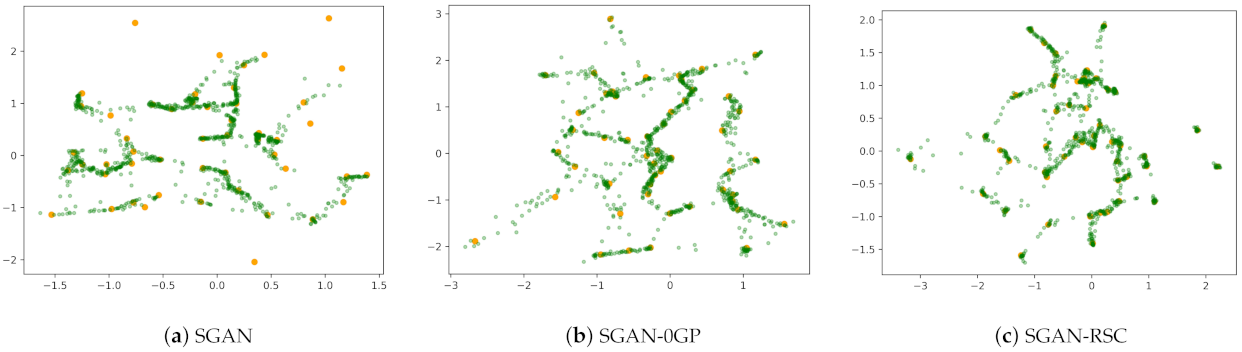
We verified our previous analysis by the experiments on the synthetic dataset. As shown in Figure 1, SGAN-0GP showed more fake real samples during the training process than SGAN. The number of fake real samples generated by SGAN with 0GP on real samples was similar to that on the linear interpolation between real and generated samples. We can also find that 0GP regularization on real samples and 0GP regularization on the linear interpolation between real and generated samples resulted in the number of fake real samples exceeding that in SGAN. These observations are consistent with our previous analysis in Section 3.
Figure 1 shows the qualitative results of SGAN, SGAN-0GP, and SGAN-RSC on the synthetic data. The ideal generation is to generate samples that cover every real sample and that every generated sample be close to the real samples. However, we note that the green generated samples did not cover part of the orange real samples in Figure 1a, which indicates that mode collapse occurred. In Figure 1b, although mode collapse did not occur, many generated samples were distributed far away from the real samples. The generation in Figure 1c was the best in the three subfigures. Not only was there no mode collapse, but there were fewer generated samples that were far away from the real samples. The consequence was consistent with Figure 2. Although the number of fake real samples in SGAN was low, mode collapse occurred. According to Figure 1 and Figure 2, the SGAN-RSC we proposed led to fewer fake real samples and generated samples that were far away from the real samples and avoided model collapse.
The quantitative results were consistent with the qualitative results in Figure 1. As shown in Table 1, the average distance obtained by our method was less than the average distance obtained by 0GP, and as the number of real samples increased, the better the improvement of our method. Our method’s improvement for 25 Gaussians was less than that for 50 Gaussians and 100 Gaussians because the 25 Gaussian dataset was simple, and the average distance was close to the ideal average distance.
4.2. CIFAR-10 and CIFAR-100
In CIFAR-10 and CIFAR-100, we set the image resolution at 32 × 32 and experimented on both the conventional network and ResNet. We set = 10, = 20 for the conventional network architecture and = 10, = 500 for ResNet, see Table A3, Table A4, Table A5 and Table A6 in the Appendix A for the details. The results are shown in Table 2.
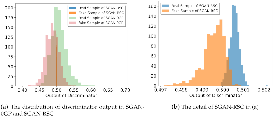
We verified our previous analysis in Section 3 by experiments on CIFAR-10 and CIFAR-100. As shown in Figure 3, the discriminator’s output with our regularization for both real samples and fake samples was more concentrated. For real samples, the proportion of the discriminator with our regularization output less than was lower than the proportion of the discriminator with 0GP regularization output less than . For fake samples, the proportion of the discriminator with our regularization output greater than was lower than the proportion of the discriminator with 0GP regularization output greater than . This was consistent with the result in Figure 2. As shown in Figure 2, the number of fake real samples in SGAN-RSC was lower than the number of fake real samples in SGAN-0GP.
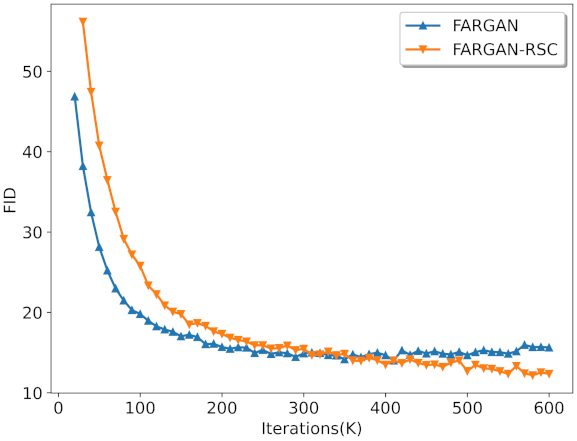
The result on FARGAN and FARGAN-RSC on CIFAR-10 is shown in Figure 4. FARGAN-RSC outperformed FARGAN. Note that the FID of FARGAN dropped quickly at the beginning of training. However, as the training progressed, the FID of FARGAN was surpassed by the FID of FARGAN-RSC, and the FID of FARGAN-RSC continued to decrease.
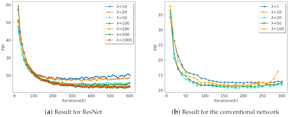
In order to obtain the optimal parameter , we selected parameter through ablation experiments, as shown in Figure 5. Figure 5a shows that, when , SGAN-RSC with ResNet achieved better results with the increase of . However, when we set , the result was worse than that of . Consequently, we set for SGAN-RSC with ResNet. Similarly, we set for SGAN-RSC with the conventional network.
To verify the effectiveness of our proposed real sample consistency regularization with different network architectures, we compared SGAN-0GP and SGAN-RSC with the conventional network and ResNet, respectively. Experiments were carried out on CIFAR-10 and CIFAR-100. The result is shown in Figure 6. In all experiments, SGAN-RSC outperformed SGAN-0GP, especially with ResNet. Note that although the FID value of SGAN-RSC with the conventional architecture on CIFAR-100 increased slowly in the late training period, and the lowest FID value of SGAN-RSC with the conventional architecture on CIFAR-100 was lower than that of SGAN-0GP with the conventional architecture on CIFAR-100. Figure 6 shows that our method was effective for different network architectures.
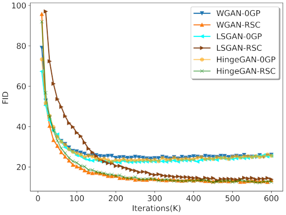
We also experimented with different GAN variants. In our experiments, 0GP on real samples instead of 1GP was applied in WGAN [16,17,31]. We set for LSGAN [19] and , and for FARGAN [15]. The result is shown in Figure 7. Note that real sample consistency regularization outperformed 0GP regularization for all GAN variants. Although LSGAN-RSC converged slowly in the early stages of training, it eventually reached an FID value similar to that obtained by other GAN variants with real sample consistency regularization. Figure 7 shows that our method was effective for different GAN variants.
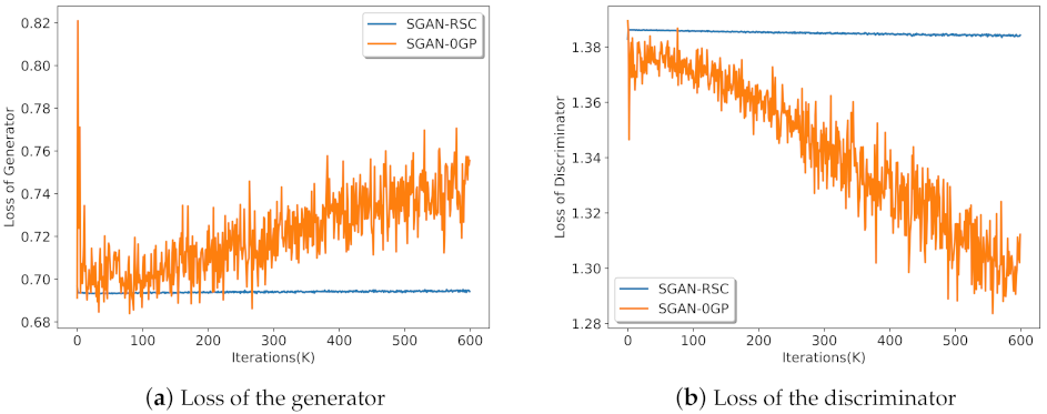
The loss of the generator and discriminator with ResNet on CIFAR-10 is shown in Figure 8. The theoretical loss was for the generator and for the discriminator. As the training progressed, we observed that the loss of the generator increased, and the loss of discriminator decreased significantly in SGAN-0GP. However, the loss of the generator and discriminator in SGAN-RSC was close to the theoretical loss and kept stable. Figure 8 shows that our method can stabilize the training of SGAN-0GP.
The qualitative result with ResNet on CIFAR-10 is shown in Figure 9. Note that the images generated by SGAN-RSC were sharper and the structure clearer, such as the images of horses, airplanes, and cars. SGAN-0GP generated more unnatural and fuzzy images due to the fake real samples. Figure 9 and Figure 10 show that our proposed regularization outperformed 0GP regularization qualitatively on CIFAR-10 and CIFAR-100. More qualitative results are shown in Figure A1, Figure A2, Figure A3 and Figure A4.
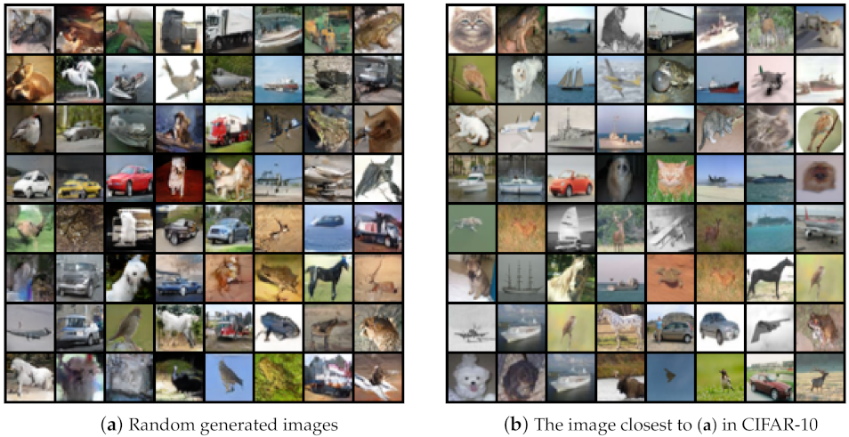
In Figure 11, we show the images randomly generated by SGAN-RSC and the images closest to the generated images in CIFAR-10. The results showed that our model did not copy the images, but learned the distribution of the real images, which can guarantee the diversity of the generation.
We compared other state-of-the-art methods, and the results are shown in Table 3. Real sample consistency regularization improved the FID score of FARGAN on CIFAR-10 from 14.28 to 9.8.
4.3. ImageNet
In order to verify the effectiveness of our method on challenging datasets, we experimented on ImageNet, which contains 1000 classes. We set the image resolution at 64 × 64 and experimented on ResNet; see Table A7 and Table A8 in the Appendix A for details. We set = 10, = 20. The results are shown in Table 4.
4.4. Summary of the Experimental Results
As shown in Table 5, the results of RSC regularization on all datasets surpassed the results of 0GP regularization. This shows that our method works for different datasets.
5. Conclusions
This paper showed that 0GP regularization introduces the discriminator’s misjudgment, which is the discriminator outputting a higher value for some generated samples than the real samples. We analyzed the discriminator’s output for the real sample, which was that a close pair with several generated samples was less than . We proposed a new regularization, which forced the discriminator to output the same value for all real samples. The experiment result showed that our proposed regularization can reduce the number of fake real samples. Experiments on synthetic data showed that our method reduces the distance between the real distribution and the generated distribution and avoids mode collapse. Experiments on CIFAR-10, CIFAR-100, and ImageNet verified that our method can stabilize the training process and significantly improve the performance.
Author Contributions
Conceptualization, J.Z.; methodology, J.Z.; software, J.Z.; validation, J.Z.; formal analysis, J.Z.; investigation, J.Z.; resources, J.Z.; data curation, J.Z.; writing—original draft preparation, J.Z.; writing—review and editing, X.Z. and J.Z.; visualization, X.Z.; supervision, X.Z.; project administration, X.Z. All authors have read and agreed to the published version of the manuscript.
Funding
This research received no external funding.
Institutional Review Board Statement
Not applicable.
Informed Consent Statement
Not applicable.
Data Availability Statement
Not applicable.
Conflicts of Interest
The authors declare no conflict of interest.
Appendix A

Table A1.
Generator architecture in the synthetic experiment.
| Layer | Output Size | Filter |
|---|---|---|
| Fully connected | 64 | 2 → 64 |
| RELU | 64 | – |
| Fully connected | 64 | 64 → 64 |
| RELU | 64 | – |
| Fully connected | 64 | 64 → 64 |
| RELU | 64 | – |
| Fully connected | 2 | 64 → 2 |
Table A2.
Discriminator architecture in the synthetic experiment.
| Layer | Output Size | Filter |
|---|---|---|
| Fully connected | 64 | 2 → 64 |
| RELU | 64 | – |
| Fully connected | 64 | 64 → 64 |
| RELU | 64 | – |
| Fully connected | 64 | 64 → 64 |
| RELU | 64 | – |
| Fully connected | 1 | 64 → 1 |
Table A3.
Generator ResNet architecture in the CIFAR experiment.
| Layer | Output Size | Filter |
|---|---|---|
| Fully connected | 512 × 4 × 4 | 128 → 512 × 4 × 4 |
| Reshape | 512 × 4 × 4 | – |
| ResNet-Block | 256 × 4 × 4 | 512 → 256 → 256 |
| NN-Upsampling | 256 × 8 × 8 | – |
| ResNet-Block | 128 × 8 × 8 | 256 → 128 → 128 |
| NN-Upsampling | 128 × 16 × 16 | – |
| ResNet-Block | 64 × 16 × 16 | 128 → 64 → 64 |
| NN-Upsampling | 64 × 32 × 32 | – |
| ResNet-Block | 64 × 32 × 32 | 64 → 64 → 64 |
| Conv2D | 3 × 32 × 32 | 64 → 3 |
Table A4.
Discriminator ResNet architecture in the CIFAR experiment.
| Layer | Output Size | Filter |
|---|---|---|
| Conv2D | 64 × 32 × 32 | 3→ 64 |
| ResNet-Block | 128 × 32 × 32 | 64 → 64 → 64 |
| Avg-Pool2D | 128 × 16 × 16 | – |
| ResNet-Block | 256 × 16 × 16 | 128 → 128 → 256 |
| Avg-Pool2D | 256 × 8 × 8 | – |
| ResNet-Block | 512 × 8 × 8 | 256 → 256 → 512 |
| Avg-Pool2D | 512 × 4 × 4 | – |
| Reshape | 512 × 4 × 4 | – |
| Conv2D | 1 | 512 × 4 × 4 → 1 |
Table A5.
Generator conventional architecture in the CIFAR experiment.
| Layer | Output Size | Filter |
|---|---|---|
| Fully connected | 512 × 4 × 4 | 128 → 512 × 4 × 4 |
| Reshape | 512 × 4 × 4 | – |
| Conv2D | 512 × 4 × 4 | 512 → 512 |
| Conv2D | 512 × 4 × 4 | 512 → 512 |
| NN-Upsampling | 512 × 8 × 8 | – |
| Conv2D | 256 × 8 × 8 | 512 →256 |
| Conv2D | 256 × 8 × 8 | 256 → 256 |
| NN-Upsampling | 512 × 16 × 16 | – |
| Conv2D | 128 × 16 × 16 | 256 →128 |
| Conv2D | 128 × 16 × 16 | 128 → 128 |
| NN-Upsampling | 128 × 32 × 32 | – |
| Conv2D | 64 × 32 × 32 | 128 →64 |
| Conv2D | 64 × 32 × 32 | 64 → 64 |
| Conv2D | 3 × 32 × 32 | 64 → 3 |
Table A6.
Discriminator conventional architecture in the CIFAR experiment.
| Layer | Output Size | Filter |
|---|---|---|
| Fully connected | 512 × 4 × 4 | 128 → 512 × 4 × 4 |
| Reshape | 512 × 4 × 4 | – |
| Conv2D | 64 × 32 × 32 | 3 → 64 |
| Conv2D | 64 × 32 × 32 | 64 → 64 |
| Conv2D | 128 × 32 × 32 | 64 → 128 |
| Avg-Pool2D | 128 × 16 × 16 | – |
| Conv2D | 128 × 16 × 16 | 128 → 128 |
| Conv2D | 256 × 16 × 16 | 128 → 256 |
| Avg-Pool2D | 256 × 8 × 8 | – |
| Conv2D | 256 × 8 × 8 | 256 → 256 |
| Conv2D | 512 × 8 × 8 | 256 → 512 |
| Avg-Pool2D | 512 × 4 × 4 | – |
| Reshape | 512 × 4 × 4 | – |
| Fully connected | 1 | 512 × 4 × 4→ 1 |
Table A7.
Generator architecture in the ImageNet experiment.
| Layer | Output Size | Filter |
|---|---|---|
| Fully connected | 1024 × 4 × 4 | 256 → 1024 × 4 × 4 |
| Reshape | 1024 × 4 × 4 | – |
| ResNet-Block | 1024 × 4 × 4 | 1024 → 1024 → 1024 |
| ResNet-Block | 1024 × 4 × 4 | 1024 → 1024 →1024 |
| NN-Upsampling | 1024 × 8 × 8 | – |
| ResNet-Block | 512 × 8 × 8 | 1024 → 512 → 512 |
| ResNet-Block | 512 × 8 × 8 | 512 → 512 →512 |
| NN-Upsampling | 512 × 16 × 16 | – |
| ResNet-Block | 256 × 16 × 16 | 512 → 256 → 256 |
| ResNet-Block | 256 × 16 × 16 | 256 → 256 →256 |
| NN-Upsampling | 256 × 32 × 32 | – |
| ResNet-Block | 128 × 32 × 32 | 256 → 128 → 128 |
| ResNet-Block | 128 × 32 × 32 | 128 → 128 →128 |
| NN-Upsampling | 128 × 64 × 64 | – |
| ResNet-Block | 64 × 64 × 64 | 128 → 64 → 64 |
| ResNet-Block | 64 × 64 × 64 | 64 → 64 →64 |
| Conv2D | 3 × 64 × 64 | 64 → 3 |
Table A8.
Discriminator architecture in the ImageNet experiment.
| Layer | Output Size | Filter |
|---|---|---|
| Conv2D | 64 × 64 × 64 | 3 → 64 |
| ResNet-Block | 64 × 64 × 64 | 64 → 64 → 64 |
| ResNet-Block | 128 × 64 × 64 | 64 → 64 →128 |
| Avg-Pool2D | 128 × 32 × 32 | – |
| ResNet-Block | 128 × 32 × 32 | 128 → 128 → 128 |
| ResNet-Block | 256 × 32 × 32 | 128 → 128 →256 |
| Avg-Pool2D | 256 × 16 × 16 | – |
| ResNet-Block | 256 × 16 × 16 | 256 → 256 → 256 |
| ResNet-Block | 512 × 16 × 16 | 256 → 256 →512 |
| NN-Upsampling | 512 × 8 × 8 | – |
| ResNet-Block | 512 × 8 × 8 | 512 → 512 → 512 |
| ResNet-Block | 1024 × 8 × 8 | 512 → 512 →1024 |
| NN-Upsampling | 512 × 4 × 4 | – |
| ResNet-Block | 1024 × 4 × 4 | 1024 → 1024 →1024 |
| ResNet-Block | 1024 × 4 × 4 | 1024 → 1024 →1024 |
| Fully connected | 1 | 1024 × 4 × 4→ 1 |
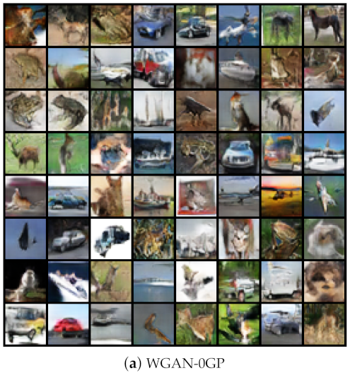
Figure A1.
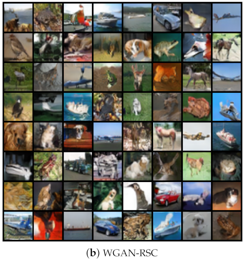
Randomly images generated by WGAN-0GP and WGAN-RSC with ResNet on CIFAR-10.


Figure A2.
Randomly images generated by HingeGAN-0GP and HingeGAN-RSC with ResNet on CIFAR-10.

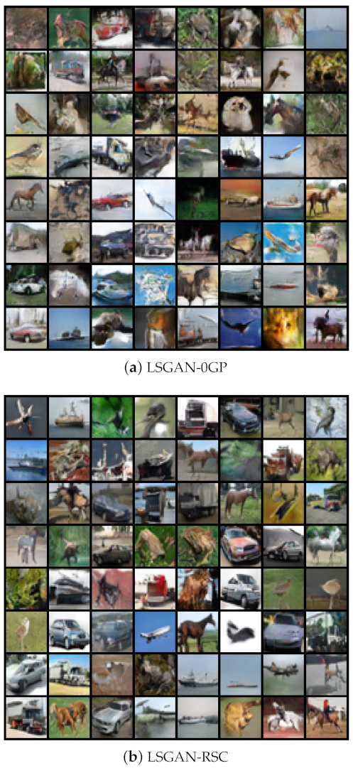
Figure A3.
Randomly images generated by LSGAN-0GP and LSGAN-RSC with ResNet on CIFAR-10.

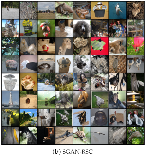
Figure A4.
Randomly images generated by SGAN-0GP and SGAN-RSC with ResNet on ImageNet.


References
- Goodfellow, I.J.; Pouget-Abadie, J.; Mirza, M.; Xu, B.; Warde-Farley, D.; Ozair, S.; Courville, A.C.; Bengio, Y. Generative Adversarial Nets. In Proceedings of the Advances in Neural Information Processing Systems, Montreal, QC, Canada, 8–13 December 2014; pp. 2672–2680. [Google Scholar]
- Jolicoeur-Martineau, A. The relativistic discriminator: A key element missing from standard GAN. In Proceedings of the International Conference on Learning Representations, New Orleans, LA, USA, 6–9 May 2019. [Google Scholar]
- Zhang, H.; Goodfellow, I.; Metaxas, D.; Odena, A. Self-Attention Generative Adversarial Networks. In Proceedings of the 36th International Conference on Machine Learning, Los Angeles, CA, USA, 10–15 June 2019; Volume 97, pp. 7354–7363. [Google Scholar]
- Gu, J.; Shen, Y.; Zhou, B. Image processing using multi-code GaN prior. In Proceedings of the IEEE Computer Society Conference on Computer Vision and Pattern Recognition, Seattle, WA, USA, 13–19 June 2020; pp. 3009–3018. [Google Scholar]
- Shen, Y.; Gu, J.; Tang, X.; Zhou, B. Interpreting the latent space of GANs for semantic face editing. In Proceedings of the IEEE Computer Society Conference on Computer Vision and Pattern Recognition, Seattle, WA, USA, 13–19 June 2020; pp. 9240–9249. [Google Scholar]
- Brock, A.; Donahue, J.; Simonyan, K. Large Scale GAN Training for High Fidelity Natural Image Synthesis. In Proceedings of the International Conference on Learning Representations, New Orleans, LA, USA, 6–9 May 2019. [Google Scholar]
- Ledig, C.; Theis, L.; Huszar, F.; Caballero, J.; Cunningham, A.; Acosta, A.; Aitken, A.; Tejani, A.; Totz, J.; Wang, Z.; et al. Photo-Realistic Single Image Super-Resolution Using a Generative Adversarial Network. In Proceedings of the IEEE Conference on Computer Vision and Pattern Recognition (CVPR), Honolulu, HI, USA, 21–26 July 2017. [Google Scholar]
- Shaham, T.R.; Dekel, T.; Michaeli, T. SinGAN: Learning a generative model from a single natural image. In Proceedings of the IEEE International Conference on Computer Vision, Seoul, Korea, 27 October–2 November 2019; pp. 4569–4579. [Google Scholar]
- Choi, Y.; Choi, M.; Kim, M.; Ha, J.W.; Kim, S.; Choo, J. StarGAN: Unified Generative Adversarial Networks for Multi-Domain Image-to-Image Translation. In Proceedings of the IEEE Conference on Computer Vision and Pattern Recognition (CVPR), Salt Lake City, UT, USA, 18–23 June 2018. [Google Scholar]
- Miyato, T.; Kataoka, T.; Koyama, M.; Yoshida, Y. Spectral normalization for generative adversarial networks. In Proceedings of the 6th International Conference on Learning Representations, ICLR 2018—Conference Track Proceedings, Vancouver, BC, Canada, 30 April–3 May 2018. [Google Scholar]
- Karras, T.; Aila, T.; Laine, S.; Lehtinen, J. Progressive Growing of GANs for Improved Quality, Stability, and Variation. In Proceedings of the International Conference on Learning Representations, Vancouver, BC, Canada, 30 April–3 May 2018. [Google Scholar]
- Karras, T.; Laine, S.; Aila, T. A Style-Based Generator Architecture for Generative Adversarial Networks. In Proceedings of the IEEE/CVF Conference on Computer Vision and Pattern Recognition (CVPR), Long Beach, CA, USA, 15–20 June 2019. [Google Scholar]
- Thanh-Tung, H.; Venkatesh, S.; Tran, T. Improving generalization and stability of generative adversarial networks. In Proceedings of the 7th International Conference on Learning Representations, ICLR 2019, New Orleans, LA, USA, 6–9 May 2019; pp. 1–18. [Google Scholar]
- Mescheder, L.; Geiger, A.; Nowozin, S. Which training methods for GANs do actually converge? In Proceedings of the 35th International Conference on Machine Learning, ICML 2018, Stockholm, Sweden, 10–15 July 2018; Volume 8, pp. 5589–5626. [Google Scholar]
- Tao, S.; Wang, J. Alleviation of gradient exploding in GANs: Fake can be real. In Proceedings of the 2020 IEEE/CVF Conference on Computer Vision and Pattern Recognition (CVPR), Seattle, WA, USA, 13–19 June 2020; pp. 1188–1197. [Google Scholar]
- Arjovsky, M.; Chintala, S.; Bottou, L. Wasserstein generative adversarial networks. In Proceedings of the 34th International Conference on Machine Learning, ICML 2017, Sydney, Australia, 6–11 August 2017; Volume 1, pp. 298–321. [Google Scholar]
- Gulrajani, I.; Ahmed, F.; Arjovsky, M.; Dumoulin, V.; Courville, A. Improved Training of Wasserstein GANs. In Proceedings of the 31st International Conference on Neural Information Processing Systems NIPS’17, Long Beach, CA, USA, 4–9 December 2017; pp. 5769–5779. [Google Scholar]
- Zhang, H.; Zhang, Z.; Odena, A.; Lee, H. Consistency Regularization for Generative Adversarial Networks. In Proceedings of the International Conference on Learning Representations, Addis Ababa, Ethiopia, 26–30 April 2020. [Google Scholar]
- Mao, X.; Li, Q.; Xie, H.; Lau, R.Y.; Wang, Z.; Smolley, S.P. Least Squares Generative Adversarial Networks. In Proceedings of the IEEE International Conference on Computer Vision, Venice, Italy, 22–29 October 2017; pp. 2813–2821. [Google Scholar]
- Wu, Y.; Liu, Y. Robust Truncated Hinge Loss Support Vector Machines. J. Am. Stat. Assoc. 2007, 102, 974–983. [Google Scholar] [CrossRef] [Green Version]
- He, K.; Zhang, X.; Ren, S.; Sun, J. Deep Residual Learning for Image Recognition. In Proceedings of the IEEE Conference on Computer Vision and Pattern Recognition (CVPR), Las Vegas, NV, USA, 27–30 June 2016. [Google Scholar]
- Sønderby, C.K.; Caballero, J.; Theis, L.; Shi, W.; Huszár, F. Amortised map inference for image super-resolution. arXiv 2017, arXiv:1610.04490. [Google Scholar]
- Klinker, F. Exponential moving average versus moving exponential average. Math. Semesterber. 2011, 58, 97–107. [Google Scholar] [CrossRef] [Green Version]
- Metz, L.; Poole, B.; Pfau, D.; Sohl-Dickstein, J. Unrolled generative adversarial networks. arXiv 2016, arXiv:1611.02163. [Google Scholar]
- Ghosh, A.; Kulharia, V.; Namboodiri, V.P.; Torr, P.H.S.; Dokania, P.K. Multi-Agent Diverse Generative Adversarial Networks. In Proceedings of the IEEE Conference on Computer Vision and Pattern Recognition (CVPR), Salt Lake City, UT, USA, 18–23 June 2018. [Google Scholar]
- Hoang, Q.; Nguyen, T.D.; Le, T.; Phung, D. MGAN: Training generative adversarial nets with multiple generators. In Proceedings of the 6th International Conference on Learning Representations, ICLR 2018—Conference Track Proceedings, Vancouver, BC, Canada, 30 April–3 May 2018; pp. 1–24. [Google Scholar]
- Arora, S.; Ge, R.; Liang, Y.; Ma, T.; Zhang, Y. Generalization and Equilibrium in Generative Adversarial Nets (GANs). In Proceedings of the 34th International Conference on Machine Learning, Sydney, Australia, 6–11 August 2017; Volume 70, pp. 224–232. [Google Scholar]
- Salimans, T.; Goodfellow, I.; Zaremba, W.; Cheung, V.; Radford, A.; Chen, X. Improved techniques for training GANs. In Proceedings of the Advances in Neural Information Processing Systems, Barcelona, Spain, 5–10 December 2016; pp. 2234–2242. [Google Scholar]
- Radford, A.; Metz, L.; Chintala, S. Unsupervised representation learning with deep convolutional generative adversarial networks. In Proceedings of the 4th International Conference on Learning Representations, ICLR 2016—Conference Track Proceedings, San Juan, PR, USA, 2–4 May 2016; pp. 1–16. [Google Scholar]
- Heusel, M.; Ramsauer, H.; Unterthiner, T.; Nessler, B.; Hochreiter, S. GANs Trained by a Two Time-Scale Update Rule Converge to a Local Nash Equilibrium. In Proceedings of the Advances in Neural Information Processing Systems, Long Beach, CA, USA, 4–9 December 2017; pp. 6629–6640. [Google Scholar]
- Petzka, H.; Fischer, A.; Lukovnikov, D. On the regularization of Wasserstein GANs. In Proceedings of the International Conference on Learning Representations, Vancouver, BC, Canada, 30 April–3 May 2018. [Google Scholar]
Figure 1.
Result of SGAN, SGAN-0GP, and SGAN-RSC on 50 Gaussians at 100 k iterations. SGAN, SAGN-0GP, and SGAN-RSC were iterated 100 k times on 50 Gaussians. The orange dots represent real samples, and the green dots represent randomly generated samples. There are 1000 green points in each subfigure.

Figure 2.
Result of the number of fake real samples in SGAN, SGAN-0GP, and SGAN-RSC with ResNet on CIFAR-10. We randomly sampled 1000 fake samples and counted the number of false samples. SGAN-0GP-R represents 0GP regularization on real samples; SGAN-0GP-I represents 0GP regularization on the linear interpolation between the real samples and the generated samples.

Figure 3.
Result of the output of discriminator in SGAN-0GP and SGAN-RSC with ResNet on CIFAR-10. We randomly sampled 1000 real samples and 1000 fake samples. The statistical discriminator’s output distribution for real samples and fake samples, respectively.
Figure 3.
Result of the output of discriminator in SGAN-0GP and SGAN-RSC with ResNet on CIFAR-10. We randomly sampled 1000 real samples and 1000 fake samples. The statistical discriminator’s output distribution for real samples and fake samples, respectively.

Figure 4.
Result on FARGAN and FARGAN-RSC on CIFAR-10 with the conventional network architecture.

Figure 5.
Result for SGAN-RSC with different on CIFAR-10 with the conventional network and ResNet.

Figure 6.
FID of SGAN-0GP and SGAN-RSC. Calculated on CIFAR-10 and CIFAR-100 with the conventional network and ResNet.
Figure 6.
FID of SGAN-0GP and SGAN-RSC. Calculated on CIFAR-10 and CIFAR-100 with the conventional network and ResNet.

Figure 7.
Result of 0GP regularization and RSC regularization on different GAN variants.

Figure 8.
The loss of the generator and discriminator in SGAN-0GP and SGAN-RSC with ResNet on CIFAR-10.
Figure 8.
The loss of the generator and discriminator in SGAN-0GP and SGAN-RSC with ResNet on CIFAR-10.

Figure 9.
Randomly images generated by SGAN-0GP and SGAN-RSC with ResNet on CIFAR-10.

Figure 10.
Randomly images generated by SGAN-0GP and SGAN-RSC with ResNet on CIFAR-100.

Figure 11.
Randomly images generated by SGAN-RSC and the image closest to it in CIFAR-10. We used the cosine distance as the basis for comparison.
Figure 11.
Randomly images generated by SGAN-RSC and the image closest to it in CIFAR-10. We used the cosine distance as the basis for comparison.

Table 1.
The average distance between the generated sample and the real samples on 25 Gaussians, 50 Gaussians, and 100 Gaussians at 100 k iterations. Experiments were repeated 10 times.
Table 1.
The average distance between the generated sample and the real samples on 25 Gaussians, 50 Gaussians, and 100 Gaussians at 100 k iterations. Experiments were repeated 10 times.
| SGAN-0GP | SGAN-RSC | |
|---|---|---|
| 25 Gaussians | 0.028 ± 0.0053 | 0.025 ± 0.0048 |
| 50 Gaussians | 0.058 ± 0.0084 | 0.048 ± 0.0102 |
| 100 Gaussians | 0.072 ± 0.0094 | 0.057 ± 0.014 |
Table 2.
FID on CIAFR-10 and CIFAR-100 with ResNet and the conventional network. Experiments were repeated 3 times.
Table 2.
FID on CIAFR-10 and CIFAR-100 with ResNet and the conventional network. Experiments were repeated 3 times.
| 0GP | RSC | |
|---|---|---|
| CIFAR-10 | ||
| ResNet SGAN | 24.15 ± 0.27 | 12.05 ± 0.50 |
| ResNet WGAN | 24.33 ± 0.16 | 12.90 ± 0.07 |
| ResNet LSGAN | 22.32 ± 0.05 | 14.40 ± 0.40 |
| ResNet HingeGAN | 23.39 ± 0.12 | 12.37 ± 0.31 |
| ResNet FARGAN | 14.28 ± 0.16 | 11.66 ± 0.09 |
| Conventional SGAN | 13.12 ± 0.41 | 10.92 ± 0.04 |
| CIFAR-100 | ||
| ResNet SGAN | 34.48 ± 0.02 | 19.80 ± 0.19 |
| Conventional SGAN | 23.42 ± 0.29 | 17.14 ± 0.07 |
Table 3.
Comparison with state-of-the-art GAN models including SNGAN [10], BigGAN [6], CR-BigGAN [18], and FARGAN [15]. The FID value of FARGAN-RSC was obtained at 1200 k iterations.
| Method | SNGAN | BigGAN | CR-BigGAN | FARGAN | FARGAN-RSC (Ours) |
|---|---|---|---|---|---|
| FID | 17.5 | 14.73 | 11.48 | 14.28 | 9.8 |
Table 4.
FID of SGAN-0GP and SGAN-RSC on ImageNet with ResNet.
| Method | SGAN-0GP | SGAN-RSC |
|---|---|---|
| FID | 53.79 | 46.92 |
Table 5.
The best results of 0GP and RSC on different datasets. On the synthetic data, we recorded the average distance between the generated sample and the real samples for comparison. On CIFAR-10, CIFAR-100, and ImageNet2012, we recorded the FID for comparison.
Table 5.
The best results of 0GP and RSC on different datasets. On the synthetic data, we recorded the average distance between the generated sample and the real samples for comparison. On CIFAR-10, CIFAR-100, and ImageNet2012, we recorded the FID for comparison.
| 0GP | RSC | |
|---|---|---|
| Synthetic data (distance) | 0.028 | 0.025 |
| CIFARA-10 (FID) | 13.12 | 9.8 |
| CIFAR-100 (FID) | 23.42 | 17.14 |
| ImageNet2012 (FID) | 53.79 | 46.92 |
Publisher’s Note: MDPI stays neutral with regard to jurisdictional claims in published maps and institutional affiliations. |
© 2021 by the authors. Licensee MDPI, Basel, Switzerland. This article is an open access article distributed under the terms and conditions of the Creative Commons Attribution (CC BY) license (https://creativecommons.org/licenses/by/4.0/).
Share and Cite
MDPI and ACS Style
Zhang, X.; Zhang, J. Real Sample Consistency Regularization for GANs. Entropy 2021, 23, 1231. https://0-doi-org.brum.beds.ac.uk/10.3390/e23091231
AMA Style
Zhang X, Zhang J. Real Sample Consistency Regularization for GANs. Entropy. 2021; 23(9):1231. https://0-doi-org.brum.beds.ac.uk/10.3390/e23091231
Chicago/Turabian StyleZhang, Xiangde, and Jian Zhang. 2021. "Real Sample Consistency Regularization for GANs" Entropy 23, no. 9: 1231. https://0-doi-org.brum.beds.ac.uk/10.3390/e23091231
Note that from the first issue of 2016, this journal uses article numbers instead of page numbers. See further details here.