
Trapezoidal-Type Inequalities for Strongly Convex and Quasi-Convex Functions via Post-Quantum Calculus


1
Department of Mathematical, Zhejiang Normal University, Jinhua 321004, China
2
Escuela de Ciencias Físicas y Matemáticas, Facultad de Ciencias Naturales y Exactas Pontificia Universidad Católica del Ecuador, Sede Quito 17-01-2184, Ecuador
3
Department of Basic Sciences, Deanship of Preparatory Year, King Faisal University, Hofuf 31982, Al-Hasa, Saudi Arabia
*
Authors to whom correspondence should be addressed.
Entropy 2021, 23(10), 1238; https://0-doi-org.brum.beds.ac.uk/10.3390/e23101238
Submission received: 30 August 2021
/
Revised: 12 September 2021
/
Accepted: 14 September 2021
/
Published: 22 September 2021
(This article belongs to the Special Issue Advanced Numerical Methods for Differential Equations)
Abstract
:In this paper, we establish new -integral and -integral identities. By employing these new identities, we establish new and - trapezoidal integral-type inequalities through strongly convex and quasi-convex functions. Finally, some examples are given to illustrate the investigated results.
1. Introduction and Preliminaries
Quantum calculus, often known as q-calculus, is a branch of mathematics that studies calculus without limits. Euler’s work on infinite series, which he integrated with Newton’s work on parameters, served as the idea for the q-calculus analysis, which was founded in the eighteenth century by famous mathematician Leonhard Euler (1707–1783). In 1910, F. H. Jackson [1] used L. Euler’s expertise to define the q-derivative and q-integral of any function on the interval using the q-calculus of infinite series. Quantum calculus has a very long history. However, to keep up with the times, it has undergone rapid growth over the past few decades. However, in order to stay current, it has experienced tremendous development over the last several decades. I am a strong believer in this as it serves as a link between mathematics and physics, which is useful when working with physics. To get more information, please check the application and results of Ernst [2], Gauchman [3], and Kac and Cheung [4] in the theory of quantum calculus and theory of inequalities in quantum calculus. In previous papers, the authors Ntouyas and Tariboon [5] investigated how quantum-derivatives and quantum-integrals are solved over the intervals of the form . In addition, they studied the characteristics and specific results of initial value problems in impulsive q-differential equations of the first and second order. Furthermore, set a number of quantum analogs for some well-known effects, for example, Hölder inequality, Hermite–Hadamard inequality and Ostrowski inequality, Cauchy–Bunyakovsky–Schwarz, Gruss, Gruss–Cebysev, and other integral inequalities that use classical convexity. Furthermore, Noor et al. [6], Sudsutad et al. [7], and Zhuang et al. [8] played an active role in the study and some integral inequalities have been established which give quantum analog for the right part of Hermite–Hadamard inequality by using q-differentiable convex and quasi-convex functions. Numerous mathematicians have carried out research in the area of q-calculus analysis; interested readers may check the works in [9,10,11,12,13,14,15,16,17,18,19].
q-calculus generalization is post-quantum or, often, is referred to as () calculus. Post-quantum calculus is a recent advancement in the study of quantum calculus that contains p and q-numbers with two independent variables p and q. Quantum calculus is concerned with q-numbers with a single basis. Therefore, ()-calculus is known as two-parameter quantum calculus. Applications play significant roles in mathematics and physics, such as combinatorics, fractals, special functions, number theory, dynamical systems, and mechanics. Many additional -analogs of classical inequalities have been discovered since the publication of this article. In ()-calculus, we get the q-calculus formula when and the original mathematical formula when . Motivated by the research work going on, Tunç and Göv [20] introduced the concepts of -derivatives and -integrals on finite intervals. Kunt et al. [21] used ()-differentiable convex and quasi-convex functions to prove the left side of the ()-Hermite–Hadamard inequality, and then generated some new ()-Hermite–Hadamard inequalities. Latif et al. [22] proved the new variations in trapezoidal inequalities after quantum have been shown to be achieved using the new -integral identity. Based on ()-calculus, many works have been published by many researchers, see in [23,24,25,26,27,28,29,30] for more details and the references cited therein.
Integral inequalities are a fundamental tool in both pure and applied mathematics for constructing qualitative and quantitative properties. This perspective facilitated the discovery of novel and significant findings in a wide variety of areas of the mathematical and engineering sciences and provided a comprehensive framework for the study of many issues. Numerous researchers have explored the different types of convex sets and convex functions.
Suppose that the function is said to be convex, if meets the following inequality:
for all and
Hermite–Hadamard inequalities are among the most well-known results in the theory of convex functional analysis. It has an intriguing geometric representation that is applicable to a wide variety of situations.
According to the exceptional inequality, if is a convex mapping on the interval I of real numbers and with . Then,
Inequality (1) was introduced by C. Hermite [31] and investigated by J. Hadamard [32] in 1893. For to be concave, both inequalities hold in the inverted direction. Many mathematicians have paid great attention to the inequality of Hermite–Hadamard due to its quality and validity in mathematical inequalities. For significant developments, modifications, and consequences regarding the Hermite–Hadamard uniqueness property and general convex function definitions, for essential details, the interested reader would like to refer to the works in [33,34,35] and references therein.
Different inequalities are used to represent convex functions. Convex functions are responsible for several well-known inequalities. Strongly convexity is a reinforcement of the concept of convexity; some aspects of strongly convex functions are just “stronger versions” of known convex properties. Polyak [36] introduced the strongly convex function as
Definition 1
Strongly convex functions play a significant role in optimization, mathematical economics, nonlinear programming, etc. Some properties of strongly convex functions are just stronger versions of properties of convex functions. Moreover, Nikodem et al. [37] introduced new characterizations of inner product spaces among normed spaces involving the notion of strong convexity.
Note that quasi-convex functions are a generalization of the convex function class, as there are quasi-convex functions that are not convex.
Definition 2
Remark 1.
The notion of strongly quasi-convexity strengthens the concept of quasi-convexity.
Latif et al. [22] proved quantum estimates of -trapezoidal integral inequalities through convex and quasi-convex functions
Theorem 1
([22]). Suppose that is a -differentiable function on , is a -integrable on and . If is a convex functions on with , then
where
Theorem 2
([22]). Suppose that is a -differentiable function on , is a -integrable on and . If is a quasi-convex functions on with , then
where
Several fundamental inequalities that are well known in classical analysis, like Hölder inequality, Ostrowski inequality, Cauchy–Schwarz inequality, Grüess–Chebyshev inequality, and Grüess inequality. Using classical convexity, other fundamental inequalities have been proven and applied to q-calculus.
Our objective is to develop improved trapezoidal type inequalities by using post-quantum calculus and to support this claim graphically.
1.1. q-Derivatives and Integrals
In this section, we discuss some required definitions of q, -Calculus and important quantum integral inequalities for Hermite–Hadamard on left and right sides bonds. Throughout this paper, we are using constants and .
The integers are known as q-integers and are written as
The and are denoted as q-factorial and q-binomial, respectively, and are written as follows:
In the early twentieth century, the Reverend Frank Hilton Jackson made major contributions to the classical concept of a derivative of a function at a point, which allowed for a more straightforward study of ordinary calculus and number theory in these investigations. Jackson is responsible for numerous seminal studies in the subject, including that in [1], in addition to creating the q-analogs of certain major results discovered in these disciplines.
The classic Jackson approach is given below.
provided the sum converge absolutely.
The q-Jackson integral in a generic interval is defined as follows:
Whenever q approaches 1, the number theory, deduction, and ordinary integration findings become polynomial expressions in a real variable q.
Definition 3
([5]). We suppose that be an arbitrary function. Then -derivative of at is defined as follows:
As is an arbitrary function from to , so for , we define . The function is called -differentiable on , if exists for all .
The following lemma is play key part to calculate -derivatives.
Lemma 1
Definition 4
([5]). We suppose that be an arbitrary function, then the -definite integral on is described as below
The following properties are very important in quantum calculus:
Theorem 3
([5]). Let be a continuous function. Then,
- 1.
- ;
- 2.
- ,
The following is useful results for evaluating such -integrals.
Lemma 2
In [9], Alp et al. established the -Hermite–Hadamard inequalities for convexity, which is defined as follows:
Theorem 4
([9]). We suppose that is a convex differentiable function on . Then -Hermite–Hadamard inequalities are as follows:
On the other hand, the following new description of -derivative, -integration and related -Hermite–Hadamard form inequalities were given by Bermudo et al. [15]
Definition 5
As is an arbitrary function from to , so for , we define . The function is called -differentiable on , if exists for all .
Definition 6
Theorem 5
([15]). We suppose that be a convex function on Then, -Hermite–Hadamard inequalities are as follows:
From Theorems 4 and 5, one can the following inequalities:
Corollary 1
1.2. (p,q)-Derivatives and Integrals
In this section, we review some fundamental notions and symbols of -calculus.
The integers are known as () integers and are written as
The and are denoted as ()-factorial and ()-binomial, respectively, and are written as follows:
Definition 7
Definition 8
As is an arbitrary function from to , so for , we define . The function is called -differentiable on , if exists for all .
Definition 9
As is an arbitrary function from to , so for , we define . The function is called -differentiable on , if exists for all .
Definition 10
Definition 11.
From [23], the definite ()-integral of mapping on is stated as
Remark 3.
If we take and in (15), then we have
Similarly, by taking and in (16), then we obtain that
In [21], Kunt et al. proved the following Hermite–Hadamard-type inequalities for convex functions via () integral:
Theorem 6
([21]). For a convex mapping which is differentiable on the following inequalities hold for -integral:
Lemma 3.
We have the following equalities:
where
Proof.
From Definition 11, we have
Similarly, we can compute the second integral by using the Definition 10, for more details see in [18]. □
The main objective of this paper is to present some new () estimates of trapezoidal type inequalities for strongly convex and quasi-convex functions and show the relationship between the results given herein. Some examples are given to illustrate the investigated results. Finally, conclusion part is given at the end.
2. Trapezoidal Type Inequalities for (p,q)-Quantum Integrals
We are now providing new trapezoidal type inequalities for functions whose absolute value of first - and -derivatives are strongly convex functions with modulus . To prove our main results, we will initially suggest the following useful lemmas.
Lemma 4.
Suppose that is a -differentiable function on . If is a -integrable on Then, the following identity holds:
Proof.
By using Definitions 8 and 10, we have
We observe that
and
Similarly,
and
Lemma 5.
Suppose that is a -differentiable function on . If is a -integrable on . Then, the following identity holds:
Proof.
The proof is directly followed by Definitions 9 and 11. We omit the details. □
Theorem 7.
If we suppose that all of the criteria of Lemma 4 are satisfied, then the resulting inequality, shows that is a strongly convex functions on with modulus for , then
where
Proof.
Taking modulus on Equation (18) and using the power-mean inequality, we have
Using the strongly convexity of on , we obtain
By using Definition 10, we get
Similarly, we also observe that
We also have
Corollary 2.
If together with the assumptions of Theorem 7, we obtain
where and are defined in Theorem 7.
Corollary 3.
As and in Theorem 7, we get the inequality
Corollary 4.
Suppose that the assumptions of Theorem 7 with and letting , we obtain the inequality
Theorem 8.
If we suppose that all of the criteria of Lemma 4 are satisfied, then the resulting inequality, shows that is a strongly convex functions on with modulus for then
where
Proof.
Taking modulus on Equation (18) and using Hölder inequality, we have
We now evaluate the integrals involved in (43). We observe that
Consider
and
Using the strongly convexity of on , we obtain
and similarly, we get
Theorem 9.
If we suppose that all of the criteria of Lemma 4 are satisfied, then the resulting inequality shows that is a strongly quasi-convex functions on with modulus for , then
where
and , are defined in Theorem 7.
Proof.
Taking modulus on Equation (18) and using the power-mean inequality, we have
Using the strongly convexity of on , we obtain
and
Corollary 5.
Letting in Theorem 9, we obtain
where
Corollary 6.
Letting in Theorem 9 together with , we obtain
where
Theorem 10.
If we suppose that all of the criteria of Lemma 5 are satisfied, then the resulting inequality, shows that is a strongly convex functions on with modulus for , then
where , , and are defined in Theorem 7.
Proof.
The desired inequality (55) can be obtained by following the strategy applied in the proof of Theorem 7 and considering the Lemma 5. □
Theorem 11.
If we suppose that all of the criteria of Lemma 5 are satisfied, then the resulting inequality shows that is a strongly convex functions on with modulus for then
where is defined in Theorem 8.
Proof.
The desired inequality (56) can be obtained by following the strategy applied in the proof of Theorem 8 and considering the Lemma 5. □
Theorem 12.
If we suppose that all of the criteria of Lemma 5 are satisfied, then the resulting inequality shows that is a strongly quasi-convex functions on with modulus for , then
where
and , are defined in Theorem 7.
Proof.
The desired inequality (57) can be obtained by following the strategy applied in the proof of Theorem 9 and considering the Lemma 5. □
3. Examples
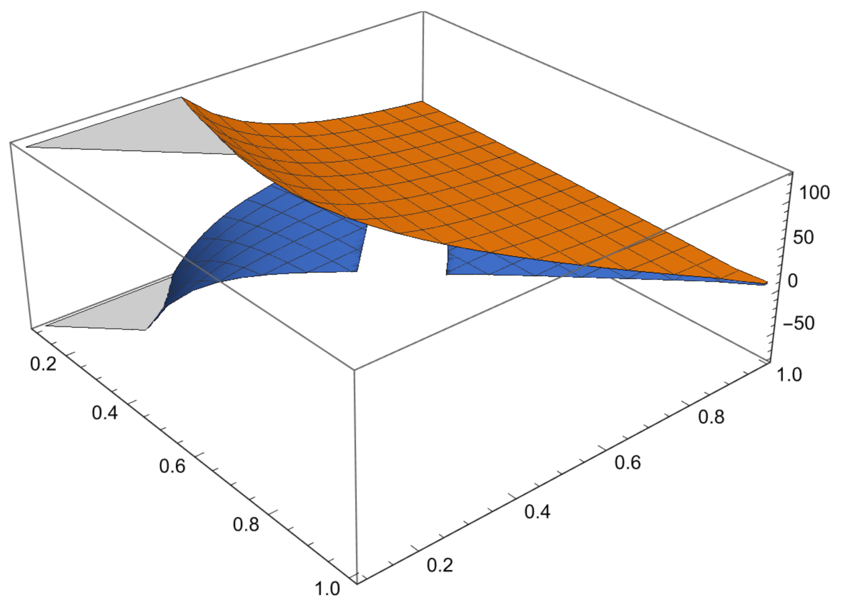
Some examples are given to illustrate the investigated results and Figure 1 shown the comparison of error and error bound in (26), Figure 2 shown the comparison of error and error bound in (42)and Figure 3 shown the comparison of error and error bound in (50), respectively.
Example 1.
Figure 1.
Comparison of error and error bound in (26).
Figure 1.
Comparison of error and error bound in (26).

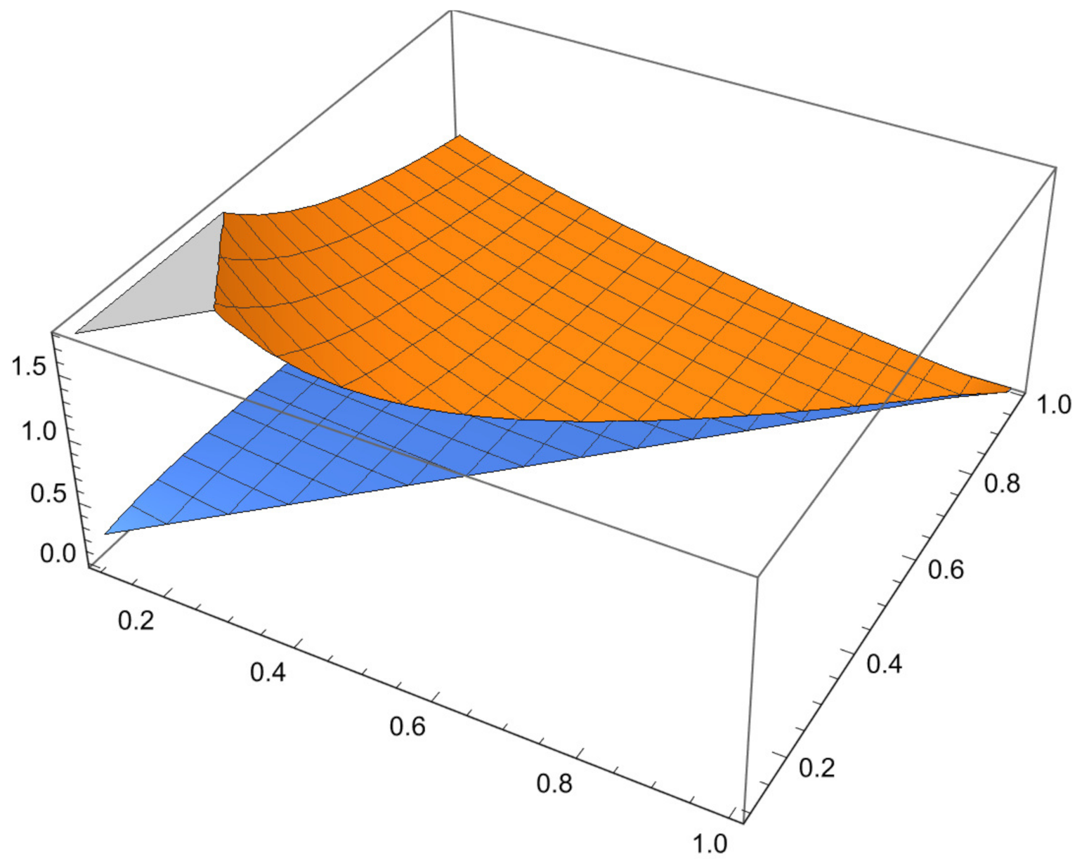
Example 2.
Consider a function by with . Then, is a strongly convex functions on Then, satisfies the conditions of Theorem 8 with , so the left side of (42) becomes
and the right side of (42) with becomes
where is defined in Theorem 8.
The series above can be shown to be convergent. The graph below shows that the LHS is less than or equal to the RHS. Therefore, the inequality (42) is valid for the particular choice of the function defined by with and , which is a strongly convex functions on
Figure 2.
Comparison of error and error bound in (42).
Figure 2.
Comparison of error and error bound in (42).

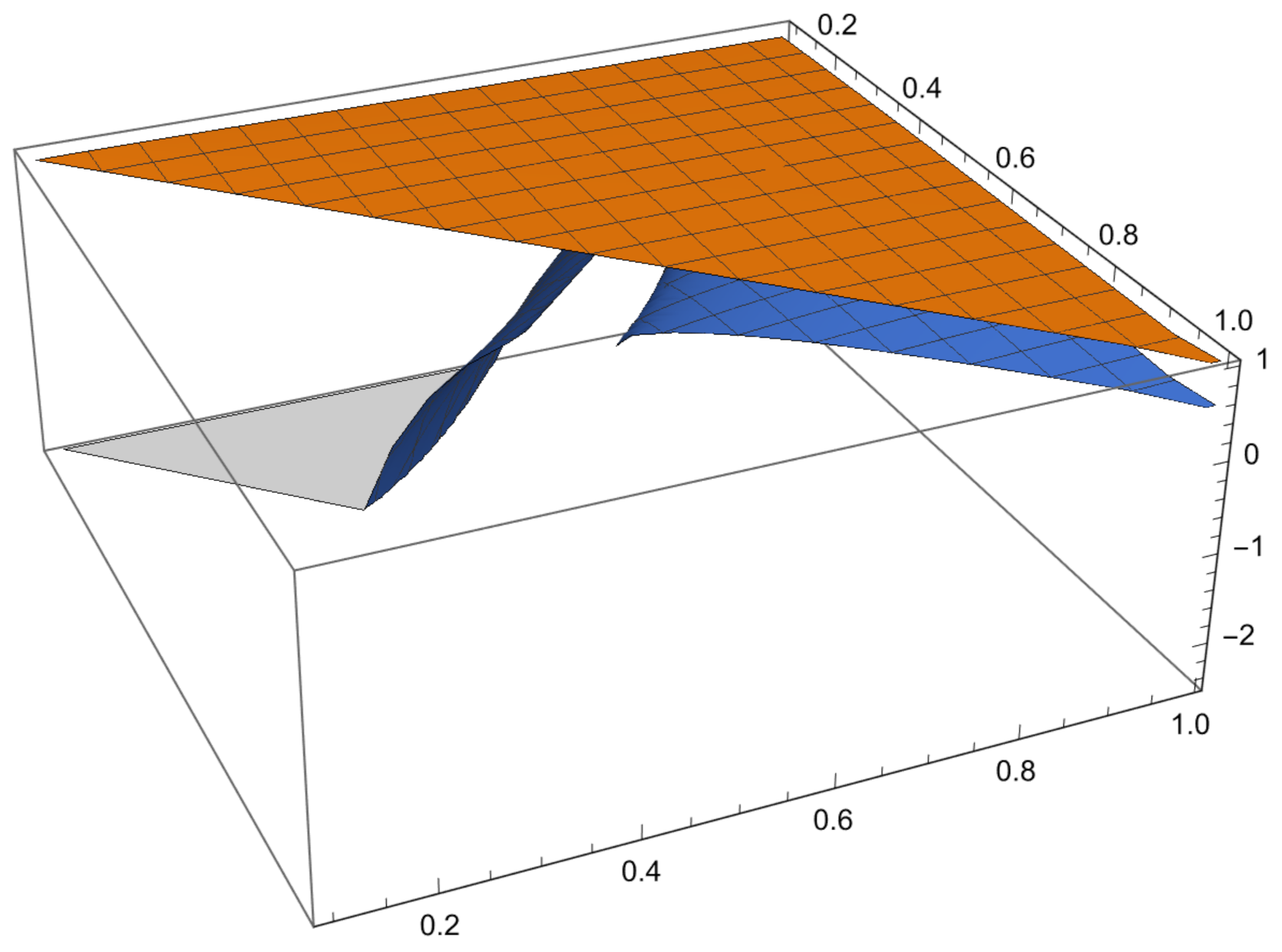
Example 3.
Consider a function by with . Then, is a strongly quasi-convex functions on . Then satisfies the conditions of Theorem 9 with , so the left side of (50) becomes
and the right side of (50) with becomes
From the graph below, it is obvious that the LHS is less than or equal to the RHS. Therefore, the inequality (50) is valid for every strongly quasi-convex functions.
Figure 3.
Comparison of error and error bound in (50).
Figure 3.
Comparison of error and error bound in (50).

4. Conclusions
Convex functions are represented in terms of different inequalities. Many of the well-known inequalities are consequences of convex functions. Strong convexity is a strengthening of the notion of convexity; some properties of strongly convex functions are just stronger versions of known properties of convex functions. In this research, we identified new results that are used to calculate and —trapezoidal integral-type inequalities through strongly convex and quasi-convex functions. Furthermore, some examples were presented to illustrate the outcome of the research.
Author Contributions
Writing—original draft, H.K.; Writing—review and editing, H.K. and M.A.L.; Formal analysis, H.K. and M.A.L.; software, H.K. and M.V.-C.; Methodology, M.A.L.; Validation, M.V.-C.; Funding acquisition, M.V.-C.; Supervision, M.A.L. All authors have read and agreed to the published version of the manuscript.
Funding
Department of Mathematical, Zhejiang Normal University, Jinhua 321004, China.
Institutional Review Board Statement
Not applicable.
Informed Consent Statement
Not applicable.
Data Availability Statement
Not applicable.
Acknowledgments
The Chinese Government is to be acknowledged for providing postdoctoral studies to Humaira Kalsoom. We want to give thanks to the Dirección de investigación from Pontificia Universidad Católica del Ecuador for technical support to our research project entitled: “Algunas desigualdades integrales para funciones convexas generalizadas y aplicaciones”.
Conflicts of Interest
The authors declare no conflict of interest.
References
- Jackson, F.H. On a q-definite integrals. Quarterly J. Pure Appl. Math. 1910, 41, 193–203. [Google Scholar]
- Ernst, T. A Comprehensive Treatment of q-Calculus; Springer: Basel, Switzerland, 2012. [Google Scholar]
- Gauchman, H. Integral inequalities in q-calculus. Comput. Math. Appl. 2004, 47, 281–300. [Google Scholar] [CrossRef] [Green Version]
- Kac, V.; Cheung, P. Quantum Calculus, Universitext; Springer: New York, NY, USA, 2002. [Google Scholar]
- Tariboon, J.; Ntouyas, S.K. Quantum calculus on finite intervals and applications to impulsive difference equations. Adv. Differ. Equ. 2013, 2013, 19. [Google Scholar] [CrossRef] [Green Version]
- Noor, M.A.; Noor, K.I.; Awan, M.U. Some quantum integral inequalities via preinvex functions. Appl. Math. Comput. 2015, 269, 242–251. [Google Scholar] [CrossRef]
- Sudsutad, W.; Ntouyas, S.K.; Tariboon, J. Quantum integral inequalities for convex functions. J. Math. Inequal. 2015, 9, 781–793. [Google Scholar] [CrossRef] [Green Version]
- Zhang, Y.; Du, T.-S.; Wang, H.; Shen, Y.-J. Different types of quantum integral inequalities via (α,m)-convexity. J. Inequal. Appl. 2018, 2018, 264. [Google Scholar] [CrossRef] [PubMed]
- Alp, N.; Kaya, M.Z.S.; Kunt, M.; İşcan, İ. q-Hermite-Hadamard inequalities and quantum estimates for midpoint type inequalities via convex and quasi-convex functions. J. King Saud Univ. Sci. 2018, 30, 193–203. [Google Scholar] [CrossRef] [Green Version]
- Khan, M.A.; Mohammad, N.; Nwaeze, E.R.; Chu, Y.-M. Quantum Hermite-Hadamard inequality by means of a Green function. Adv. Differ. Equ. 2020, 2020, 99. [Google Scholar] [CrossRef]
- Kalsoom, H.; Rashid, S.; Idrees, M.; Baleanu, D.; Chu, Y.M. Two-variable quantum integral inequalities of Simpson-type based on higher-order generalized strongly preinvex and quasi-preinvex functions. Symmetry 2020, 12, 51. [Google Scholar] [CrossRef] [Green Version]
- Deng, Y.; Kalsoom, H.; Wu, S. Some new quantum Hermite–Hadamard-type estimates within a class of generalized (s, m)-preinvex functions. Symmetry 2019, 1, 1283. [Google Scholar] [CrossRef] [Green Version]
- Kalsoom, H.; Wu, J.D.; Hussain, S.; Latif, M.A. Simpson’s type inequalities for co-ordinated convex functions on quantum calculus. Symmetry 2019, 11, 768. [Google Scholar] [CrossRef] [Green Version]
- Wang, H.; Kalsoom, H.; Budak, H.; Idrees, M. q-Hermite–Hadamard Inequalities for Generalized Exponentially (s, m, η)-Preinvex Functions. J. Math. 2021, 2021, 5577340. [Google Scholar] [CrossRef]
- Bermudo, S.; Kórus, P.; Valdés, J.N. On q-Hermite–Hadamard inequalities for general convex functions. Acta Math. Hung. 2020, 162, 364–374. [Google Scholar] [CrossRef]
- Kalsoom, H.; Idrees, M.; Baleanu, D.; Chu, Y.M. New Estimates of q1q2-Ostrowski-Type Inequalities within a Class of-Polynomial Prevexity of Functions. J. Funct. Spaces 2020, 2020, 3720798. [Google Scholar] [CrossRef]
- You, X.; Kara, H.; Budak, H.; Kalsoom, H. Quantum Inequalities of Hermite—Hadamard Type for r-Convex Functions. J. Math. 2021, 2021, 6634614. [Google Scholar] [CrossRef]
- Vivas-Cortez, M.; Ali, M.A.; Budak, H.; Kalsoom, H.; Agarwal, P. Some New Hermite–Hadamard and Related Inequalities for Convex Functions via (p, q)-Integral. Entropy 2021, 23, 828. [Google Scholar] [CrossRef]
- Chu, H.; Kalsoom, H.; Rashid, S.; Idrees, M.; Safdar, F.; Chu, Y.M.; Baleanu, D. Quantum Analogs of Ostrowski-Type Inequalities for Raina’s Function correlated with Coordinated Generalized Φ-Convex Functions. Symmetry 2020, 12, 308. [Google Scholar] [CrossRef] [Green Version]
- Tunç, M.; Göv, E. Some integral inequalities via (p,q)-calculus on finite intervals. RGMIA Res. Rep. Coll. 2016, 19, 1–12. [Google Scholar]
- Kunt, M.; İ.şcan, I.; Alp, N.; Sarikaya, M.Z. (p,q)-Hermite-Hadamard inequalities and (p,q)-estimates for midpoint type inequalities via convex and quasi-convex functions. Rev. R. Acad. Cienc. Exactas Fís. Nat. Ser. A Mat. RACSAM 2018, 112, 969–992. [Google Scholar] [CrossRef]
- Latif, M.A.; Kunt, M.; Dragomir, S.S. Post-quantum trapezoid type inequalities. Aims Math. 2020, 5, 4011–4026. [Google Scholar] [CrossRef]
- Chu, Y.-M.; Awan, M.U.; Talib, S.; Noor, M.A.; Noor, K.I. New post quantum analogues of Ostrowski-type inequalities using new definitions of left–right (p,q)-derivatives and definite integrals. Adv. Differ. Equ. 2020, 634, 1–15. [Google Scholar] [CrossRef]
- Prabseang, J.; Nonlaopon, K.; Tariboon, J.; Ntouyas, S.K. Refinements of Hermite-Hadamard Inequalities for Continuous Convex Functions via (p,q)-Calculus. Mathematics 2021, 9, 446. [Google Scholar] [CrossRef]
- Klasoom, H.; Minhyung, C. Trapezoidal (p,q)-Integral Inequalities Related to (η1,η2)-convex Functions with Applications. Int. J. Theor. Phys. 2021, 60, 2627–2641. [Google Scholar] [CrossRef]
- Kalsoom, H.; Amer, M.; Junjua, M.U.; Hussain, S.; Shahzadi, G. Some (p,q)-estimates of Hermite-Hadamard-type inequalities for coordinated convex and quasi-convex functions. Mathematics 2019, 7, 683. [Google Scholar] [CrossRef] [Green Version]
- Kalsoom, H.; Latif, M.A.; Rashid, S.; Baleanu, D.; Chu, Y.M. New (p,q)-estimates for different types of integral inequalities via (α,m)-convex mappings. Open Math. 2020, 18, 1830–1854. [Google Scholar] [CrossRef]
- Kalsoom, H.; Idrees, M.; Kashuri, A.; Awan, M.U.; Chu, Y.M. Some new (p1p2,q1q2)-estimates of Ostrowski-type integral inequalities via n-polynomials s-type convexity. AIMS Math 2020, 5, 7122–7144. [Google Scholar] [CrossRef]
- Usman, T.; Saif, M.; Choi, J. Certain identities associated with (p,q)-binomial coefficients and (p,q)-Stirling Polynomials of the second kind. Symmetry 2020, 12, 1436. [Google Scholar] [CrossRef]
- Kalsoom, H.; Ali, M.A.; Idrees, M.; Agarwal, P.; Arif, M. New Post Quantum Analogues of Hermite–Hadamard Type Inequalities for Interval-Valued Convex Functions. Math. Probl. Eng. 2021, 17, 5529650. [Google Scholar]
- Hermite, C. Sur deux limites d’une intégrale dé finie. Mathesis 1883, 3, 82. [Google Scholar]
- Hadamard, J. Etude sur les propri etes des fonctions enteres et en particulier dune fonction Consideree par Riemann. J. Math. Pures Appl. 1893, 58, 171–215. [Google Scholar]
- Dragomir, S.S.; Agarwal, R.P. Two inequalities for differentiable mappings and applications to special means of real numbers and to trapezoidal formula. Appl. Math. Lett. 1998, 11, 91–95. [Google Scholar] [CrossRef] [Green Version]
- Kalsoom, H.; Hussain, S.; Rashid, S. Hermite-Hadamard type integral inequalities for functions whose mixed partial derivatives are co-ordinated preinvex. Punjab Univ. J. Math. 2020, 52, 63–76. [Google Scholar]
- Kalsoom, H.; Hussain, S. Some Hermite-Hadamard type integral inequalities whose n-times differentiable functions are s-logarithmically convex functions. Punjab Univ. J. Math. 2019, 2019, 65–75. [Google Scholar]
- Polyak, B.T. Existence theorems and convergence of minimizing sequences in extremum problems with restrictions, Soviet mathematics. Doklady 1966, 166, 72–75. [Google Scholar]
- Nikodem, K.; Pales, Z.S. Characterizations of inner product spaces by strongly convex functions. Banach J. Math. Anal. 2011, 1, 83–87. [Google Scholar] [CrossRef]
- Ion, D.A. Some estimates on the Hermite-Hadamard inequality through quasi-convex functions. Ann. Univ. Craiova Ser. Mat. Inform. 2007, 34, 83–88. [Google Scholar]
Publisher’s Note: MDPI stays neutral with regard to jurisdictional claims in published maps and institutional affiliations. |
© 2021 by the authors. Licensee MDPI, Basel, Switzerland. This article is an open access article distributed under the terms and conditions of the Creative Commons Attribution (CC BY) license (https://creativecommons.org/licenses/by/4.0/).
Share and Cite
MDPI and ACS Style
Kalsoom, H.; Vivas-Cortez, M.; Latif, M.A. Trapezoidal-Type Inequalities for Strongly Convex and Quasi-Convex Functions via Post-Quantum Calculus. Entropy 2021, 23, 1238. https://0-doi-org.brum.beds.ac.uk/10.3390/e23101238
AMA Style
Kalsoom H, Vivas-Cortez M, Latif MA. Trapezoidal-Type Inequalities for Strongly Convex and Quasi-Convex Functions via Post-Quantum Calculus. Entropy. 2021; 23(10):1238. https://0-doi-org.brum.beds.ac.uk/10.3390/e23101238
Chicago/Turabian StyleKalsoom, Humaira, Miguel Vivas-Cortez, and Muhammad Amer Latif. 2021. "Trapezoidal-Type Inequalities for Strongly Convex and Quasi-Convex Functions via Post-Quantum Calculus" Entropy 23, no. 10: 1238. https://0-doi-org.brum.beds.ac.uk/10.3390/e23101238
Note that from the first issue of 2016, this journal uses article numbers instead of page numbers. See further details here.