
Simple Equations Method and Non-Linear Differential Equations with Non-Polynomial Non-Linearity


1
Institute of Mechanics, Bulgarian Academy of Sciences, Acad. G. Bonchev Str., Block 4, 1113 Sofia, Bulgaria
2
Climate, Atmosphere and Water Research Institute, Bulgarian Academy of Sciences, Blvd. Tzarigradsko Chaussee 66, 1784 Sofia, Bulgaria
*
Author to whom correspondence should be addressed.
Entropy 2021, 23(12), 1624; https://0-doi-org.brum.beds.ac.uk/10.3390/e23121624
Submission received: 6 November 2021
/
Revised: 27 November 2021
/
Accepted: 29 November 2021
/
Published: 2 December 2021
(This article belongs to the Special Issue Advanced Numerical Methods for Differential Equations)
Abstract
:We discuss the application of the Simple Equations Method (SEsM) for obtaining exact solutions of non-linear differential equations to several cases of equations containing non-polynomial non-linearity. The main idea of the study is to use an appropriate transformation at Step (1.) of SEsM. This transformation has to convert the non-polynomial non- linearity to polynomial non-linearity. Then, an appropriate solution is constructed. This solution is a composite function of solutions of more simple equations. The application of the solution reduces the differential equation to a system of non-linear algebraic equations. We list 10 possible appropriate transformations. Two examples for the application of the methodology are presented. In the first example, we obtain kink and anti- kink solutions of the solved equation. The second example illustrates another point of the study. The point is as follows. In some cases, the simple equations used in SEsM do not have solutions expressed by elementary functions or by the frequently used special functions. In such cases, we can use a special function, which is the solution of an appropriate ordinary differential equation, containing polynomial non-linearity. Specific cases of the use of this function are presented in the second example.
1. Introduction
Complex systems are numerous in human societies and in Nature. Several examples are research groups, communities, traffic networks, stock markets, etc. [1,2,3,4,5,6,7,8]. The above (and many other) complex systems are important. Because of this, their dynamics are studied by many research groups [9,10,11,12,13,14,15,16,17,18,19,20,21,22,23]. Characteristic feature of the most complex systems is their non-linearity. Examples for this can be seen in fluid mechanics, solid state physics, etc. [24,25,26,27,28,29,30,31]. In many cases, the non-linearity is modeled by non-linear differential or difference equations [32,33,34,35,36,37,38,39,40,41,42,43,44,45,46,47,48,49]. Thus, the study of the analytical and numerical solutions of the non-linear differential equations are of large interest for science and for practice. We note that the exact solutions of nonlinear differential equations are of interest also for the numerical analysis of these equations. The reason is that the exact solutions can be used to test the corresponding numerical methods and computer programs.
The research on the exact solutions of the non-linear differential equation started a long time ago. At the beginning, the efforts were directed at removing the non-linearity of the solved equation by means of an appropriate transformation. A large success in this direction was the Hopf–Cole transformation [50,51]. It transforms the non-linear Burgers equation to the linear heat equation. An even larger success was the transformation which connected the Korteweg–de Vries equation to the famous linear equation of Schrödinger. This transformation leaded to the development of t the Method of Inverse Scattering Transform [52,53,54]. Another method which uses an appropriate transformation is the method of Hirota [55,56]. Truncated Painleve expansions lead to many of these appropriate transformations [57,58,59,60,61].
Below, we discuss the SEsM (Simple Equations Method) for obtaining exact solutions of non-linear differential equations. Before the arising of SEsM, Kudryashov formulated the Method of Simplest Equation (MSE) [62]. MSE is based on the determination of the singularity order n of the solved NPDE and on searching of a particular solution of this equation as a series containing powers of solutions of a simpler equation called the simplest equation [63,64,65,66]). Kudryashov [67,68,69,70] also used various transformations in order to transform the non-linearity of a generalized evolution equation of the wave dynamics and to obtain exact solutions of this equation. More results connected to the application of the MSE can be seen, for example, in [71,72,73,74,75,76,77].
Some elements of SEsM [77,78,79,80,81] can be seen in our publications written years ago [82,83,84,85,86,87,88]. About 10 years ago [89,90], we used the ordinary differential equation of Bernoulli as the simplest equation [91] and applied a methodology called the Modified Method of Simplest Equation (MMSE) to model non-linear partial differential equations from ecology and population dynamics [92]. We have used the concept of the balance equation, which helps us to determine the kind of the simplest equations in the MMSE. The balance equation also helps us to determine the form of the solution of the solved equations as a series of the solution of the simplest equation [93,94]. The methodology based on the truncation of the series of solutions of the simplest equation by means of application of a balance equation is equivalent to the MSE mentioned above. We made many applications of MMSE for obtaining exact solutions of different non-linear differential equations [95,96,97,98,99,100,101,102,103]. We note the article [102] which is connected to the part of the topics discussed below in the text.
Over the course of the years, MMSE was extended to SEsM [77]. SEsM is connected to the possibility of using more than one simple equation in order to construct the solution of the solved non-linear differential equation. A realization of this possibility was shown in [104]. The first description of SEsM was made in [78] and then in [77,79,80,81,105]. Several examples of the methodology and its applications are presented in [106,107,108,109,110,111]. An important part of SEsM is the construction of the solution of the solved equation. This solution is a composite function of solutions of more simple differential equations. Thus, the Faa di Bruno formula for the derivative of the composite function participates in the process of obtaining exact solutions [112,113]. The possibility for use of more than one simple equation and the possibility of use complicated composite functions which connect the solution of the solved equation and the solutions of the simple equation distinguish SEsM from the methodology of Kudryashov and from other methodologies such as the Modified Simple Equation Method [114,115]. We note also that SEsM can be easily connected to other approaches (for examples, see [116,117,118]).
Up to now, SEsM can deal successfully with many non-linear differential equations which contain polynomial non-linearity. In this article, we start to study the topic of the application of SEsM to non-linear differential equations with non-polynomial non-linearity. Our approach will be similar to many of the approaches described above. We will search for appropriate transformations. These transformations will transform the non-polynomial non-linearity of the solved equations to polynomial non-linearity. After this, we will use the capacity of the SEsM to obtain exact analytical solutions of many equations containing polynomial non-linearity.
The text below is organized as follows. We describe the SEsM in Section 2. We note that the general case of the SEsM is for a system of non-linear differential equations. Below, we consider the specific case of search for exact traveling wave solutions of one non-linear differential equation. In Section 3, we discuss the properties of the appropriate transformations and formulate two propositions about these properties. Several appropriate transformations are listed. In Section 4, we present two selected examples of application of SEsM to non-linear differential equations with non-polynomial non-linearity. The first example illustrates the reduction of the solved non-linear differential equation to a system of non-linear algebraic equations containing relationships between the parameters of the solved equation and the parameters of the constructed solution. The second example illustrates the fact that there are simple equations in the SEsM for which solutions cannot be constructed by elementary functions or by the known special functions. Because of this, we emphasize the usefulness of a special function, which is a solution of an ordinary differential equation containing polynomial non-linearity. This function plays important role in the construction of many solutions of non-linear differential equations by means of SEsM. Several concluding remarks are summarized in Section 5. The text ends with two appendices. Appendix A gives the necessary information about the derivatives of the composite functions. Appendix B supplies useful information connected to the use of composite functions and their derivatives in SEsM.
2. The Simple Equations Method (SEsM)
In general, the SEsM is designed for obtaining exact solutions of systems of differential equations. Below, we are going to discuss the specific case when one wants to obtain exact solutions of a single nonlinear differential equation. The summary of this specific case of SEsM is as follows—Figure 1. We consider the (partial or ordinary) differential equation:
In (1), depends on the function and some of its derivatives (u can be a function of several spatial coordinates). In order to obtain an exact solution of (1), we make the following four steps.
- Step (1.)
- Transformation of the non-linearity of the solved equationWe apply the following transformations:is a function of another functions , . is a function of several spatial variables as well as of the time. The transformation T may remove some non-linearity if possible. An example of such a transformation is the Hopf–Cole transformation which leads to the linearization of the Burgers equation [50,51]). Moreover, T may transform the non-linearity of the solved differential equations to a more treatable kind of non-linearity. Transformations with this property will be discussed below in the text.In numerous cases, one may skip this step (then we have ). In many other cases, the transformation is needed for obtaining a solution of the studied non-linear PDE. The application of (2) to (1) leads to non-linear differential equations for the functions . We do not know the general form for the transformation T. The reason is that the non-linearity in the solved equations can be of different kinds.We note that Step (1.) of SEsM will be at the focus of our study in this article. We are going to study non-linear equations for which non-linearity can be reduced to polynomial non-linearity by means of appropriate transformations.
- Step (2.)
- The solution is searched as composite function of solutions of more simple equationsIn this step, the functions are chosen as composite functions of functions , which are solutions of more simple differential equations. In general, we do not fix the relationship for the composite function. Then, we use the general Faa di Bruno relationship for the derivatives of a composite function [113]. In MMSE, we have used a fixed relationship for the composite function. For an example, for the case of 1 solved equation and one function F:
- Step (3.)
- Selection of the simple equationsWe select the simple equations for the functions . In addition, we have to fix the relationship between the composite functions and the functions . We note that the fixation of the simple equations and the fixation of the relationships for the composite functions are connected. The reason for this is as follows. The fixations transform the left-hand sides of the solved equations. The result of this transformation can be functions which are sums of terms. Each term contains some function multiplied by a coefficient. The coefficient is a relationship connecting some of the parameters of the solved equations and some of the parameters of the solutions of the used simple equations. Each coefficient must have at least two terms (Otherwise, the trivial solution will be produced). In order to ensure this, a balance procedure must be applied. This balance procedure leads to one or more additional relationships among the parameters of the solved equation and parameters of the solutions of the used simple equations. The additional relationships are called balance equations. The balance equations are the connection between the choice of the simple equation and the fixation of the form of the composite function.
- Step (4.)
- Solution of the obtained system of non-linear algebraic equationsWe may obtain a nontrivial solution of (1) if all coefficients mentioned in Step (3.) are set to 0. This condition leads to a system of non-linear algebraic equations. The equations connect the coefficients of the solved non-linear differential equation and for the coefficients of the solutions of the simple equations. Any nontrivial solution of this algebraic system leads to a solution of the studied non-linear partial differential equation.There are two possibilities for the solution of the system of non-linear algebraic equations:
- The number which is the sum of the number of parameters of the solution and the number of parameters of the equation can be larger than the number of algebraic equations or equal to the number of algebraic equations. Then, the system usually (but not in all of the cases) has a nontrivial solution(s). Independent parameters may be presented in this situation. The other parameters of the solution are functions of these independent parameters.
- The number which is the sum of the number of parameters of the solution and the number of parameters of the equation is smaller than the number of algebraic equations. Then, the system of algebraic equations usually does not have a nontrivial solution. However, there can be important exceptions to this. An exception occurs when the number of equations of the algebraic system can be reduced and this number becomes less or equal to the number of available parameters. Then, this case is reduced to the previous one and a nontrivial solution is possible.
3. Several Transformations Which Are of Interest for the SEsM
3.1. General Considerations
Below, we discuss in more detail the application of Step (1.) of the SEsM to differential equations containing non-polynomial non-linearity. The idea is to reduce the non-polynomial non-linearity to polynomial non-linearity and then to deal with the polynomial non-linearity by means of Steps (2.), (3.), and (4.) of the SEsM.
We consider below the problem of searching for exact solutions of non-linear differential equations containing the function and its derivatives. In general, we consider the case of several spatial variables and the time t.
Proposition 1.
Let us consider a differential equation for the function which contains terms of two kinds:
- Terms containing only derivatives of u;
- Terms containing one or several non-polynomial non-linearities of the function u and these non-polynomial non-linearity are of the same kind.
Let be a transformation with the following properties:
- Property 1: The transformation T transforms any of the non-polynomial non-linearity to a function which contains only polynomials of F.
- Property 2: The transformation T transforms the derivatives of u to terms containing only polynomials of derivatives of F or polynomials of derivatives of F multiplied or divided by polynomials of F.
Then, the transformation T transforms the studied differential equation to a differential equation containing only polynomial non-linearity of F.
Proof.
The studied differential equation contains two kinds of terms: derivatives of u and terms which contain the non-polynomial non-linearity of u. These non-polynomial non-linearities are of the same kind. Let us apply the transformation to the terms of our differential equation. We consider first each of the terms containing derivatives. According to Property 2 of the transformation T, it transforms this term to a term containing derivatives of F and polynomials of F. What remains are the terms containing the non-polynomial non-linearity. Because of the property 1 of the transformation T, each of these terms are transformed to a term containing only polynomials of F. Then, the transformation T transforms the studied differential equation for u to a differential equation containing only polynomials of F as well as derivatives of F. □
3.2. Several Kinds of Non-Linearity Possessing the Properties 1 and 2 from the Proposition above
Let us now consider several transformations which have the properties discussed in the above Proposition. We note that there are more transformations of the desired kind than the transformations listed below, and one of them will be used in the Example 2 in the next Section.
- Case 1:
- ;In this case, the transformation is . Let us consider first the case . The transformation has Property 1 as follows:The transformation has also Property 2. For an example:The derivative of u contains only a derivative of F in the nominator and a polynomial of F in the denominator. We note that further differentiation does not change the situation. For an example:Next, we consider the case . In this case, . The transformation has Property 1. In addition, the transformation that has Property 2 as the relationship also holds. Thus, the transformation works also for the non-linearity of the kind .
- Case 2:
- ; .In this case, a possible transformation is . Let us consider first the case . The transformation has Property 1 as follows:is transformed to a function which contains only polynomials of F. The transformation also has Property 2, for an example:Next, we consider the case . In this case, the transformation has Property 1 as follows:The last relationship shows that is transformed to a function containing only polynomials of F. Since , Property 2 holds.
- Case 3:
- ; .We consider first the case . The transformation is . The transformation has Property 1 as follows:The transformation also has Property 2 as follows:For the case , the transformation has Property 1 as follows:The transformation also has Property 2.
- Case 4:
- ; .We first consider the case . In this case, a possible transformation is . The non-linearity is transformed to a polynomial of F: . The derivative of u is also reduced to a relationship containing the polynomial of F and a derivative of F. For an example:For the case , is transformed to the polynomial . The derivative of u remains as above.
- Case 5:
- ; .The transformation in this case is . The non-linearity is transformed to a polynomial of F: . The derivative of u is reduced to a relationship containing a polynomial of F and a derivative of F. For an example:For the case , is transformed to the polynomial . The derivative of u remains as above.
- Case 6:
- ; .In this case, the transformation is . The derivatives of u contain derivatives of F and polynomials of F. For an example:The non-linearity is reduced as a relationship containing polynomial non-linearity of F. For the case we obtain:For the case we obtain:
- Case 7:
- ; .In this case, the transformation is . For the case :The transformation also has Property 2, for an example:For the case , the transformation has the Property 1 as follows:
- Case 8:
- ; .In this case, the transformation is . is reduced to , which is a polynomial of F. The derivatives of u contains polynomials of F and derivatives of F. For an example:
- Case 9:
- ; .In this case, the transformation is . is reduced to , which is a polynomial of F. The derivatives of u contains polynomials of F and derivatives of F. For an example:
- Case 10:
- ; .In this case, we can use the following relationships:The transformation is . The case has Property 1 as follows:As above, the transformation has Property 2. For the case :
The list of the appropriate transformations can be continued. Let us now consider two examples.
4. Two Illustrative Examples
4.1. Example 1
We consider the following equation:
where are parameters. Following the considerations from the previous section, we use the transformation at the first step of the application of the SEsM. This transformation leads to the following equation for , containing only polynomial non-linearities:
Step (2.) of the SEsM requires F to be a composite function of more simple functions: . In order to consider the general case, we have to use the information from Appendices 1 and 2. In order to keep the example relatively simple, we will consider a particular case of the above composite function:
where and . This means that we are going to search for standing wave solutions of (6). (8) leads to large simplifications of the corresponding Faa di Bruno formulas. The result is a differential equation which contains polynomials constructed of , , and their derivatives.
At Step (3.) of the SEsM, we have to determine the form of the functions and . Following the methodology of SEsM, we assume that and are solutions of more simple (and ordinary) differential equations which contain polynomial non-linearity.
where and are parameters. The simple equations are ordinary differential equations containing polynomial non-linearity. These equations are particular cases of the Equation (A7).
We substitute (9) in the relationship which occurs in Step (2.) of the SEsM. As a result, we obtain a polynomial of and , which contains monomials of and and monomials which are combinations of powers of and . These monomials are multiplied by coefficients which are non-linear algebraic relationships containing the parameters of the solved equation and the parameters of the more simple equations (9). We have to ensure that any of these non-linear algebraic relationships contains at least two terms. This is performed by a balance procedure which leads to the fixation of the values of the parameters and . Below, we consider a specific case: the case when . For this case:
In order to keep the example simple, we further restrict the form of the simple equations by setting , and in addition, we assume as well as . In such a way, the simple equations for the function and become:
The form (11) of the simple equations lead to the following system of non-linear algebraic equations (these are the non-linear algebraic relationships for the coefficients of the polynomial containing , , and their derivatives:
The system (12) has the following solution:
and v, A, l, b, d, , are free parameters (they have to satisfy the condition . Equation (13) corresponds to the following solution of (6):
This solution describes traveling waves of kind kink and anti-kink—Figure 2
4.2. Example 2
By this example, we are going to illustrate the use of a transformation which transforms non- polynomial non-linearity to polynomial non-linearity and is not listed in Section 3. In addition, we illustrate the fact that in many cases, the solutions of the more simple equations cannot be composed by elementary functions. Because of this, we will need an appropriate special function. Such a function will be discussed below.
Let us consider the following equation:
where are parameters. In order to keep the calculations simple, we will consider the case of traveling waves with the corresponding coordinate . At Step (1.) of the SEsM, we apply the following transformation:
The transformation (16) leads to the following equation for F:
Next, we have to construct F by functions which are solutions of more simple differential equations. We note the following. In [102], we mentioned a function which is the solution of the following equation with polynomial non-linearity:
where are integers. This function was denoted as where:
- ;
- k: order of derivative of g;
- l: degree of derivative in the defining ODE;
- m: highest degree of the polynomial of g in the defining ODE.
The function V has very interesting properties. Its particular cases are the trigonometric, hyperbolic, elliptic functions of Jacobi, etc. The polynomial non-linearity in the the defining Equation (18) makes the function V very convenient for use in the SEsM. For more information about the use of the function V in the SEsM, see Appendix B.
Below, we will illustrate the use of the function , which is solution of the following equation:
We note that (17) is a specific case of (19), and then the solution of (15) can be written as follows:
Let . Then, (15) becomes:
The corresponding equation for F is:
Equation (21) has the following solution:
We note that (22) can be written as:
This can be further transformed to:
Equation (25) is not an equation for any of the three main Jacobi elliptic functions. The equations for the three main Jacobi elliptic functions are ( is the modulus of the corresponding Jacobi elliptic function. ):
- : ;
- : ;
- : ;
Let us now obtain another solution of (17). At Step (2.) of the SEsM, we have to relate the composite function F to a function G, which is a function of a more simple equation. The more simple equation will be of the kind (19), namely:
where are parameters. The substitution of (26) in (17) leads to an equation for the form of the composite function. The form of the composite function is determined by the requirement that all of the coefficients of the resulting polynomial of G must have at least two terms. This requirement leads to a balance equation. This equation determines the maximum power of the polynomial of G in the relationship for the composite function F. The result of this operation for the simple Equation (26) is as follows:
The substitution of (26) and (27) in (17) leads to the following system of non-linear algebraic equations which connect the parameters of the solved equation and the parameters of the selected solution:
Above . One solution of the system (28) is:
Thus, we have obtained the following result. We obtain a solution of (17). This solution is a composite function containing the solution of Equation (26). The solution (26) can be written in terms of the V function:
Then, from (23):
The solution of (17) is as follows:
The above shows that the function V can be very useful for use in the methodology of the SEsM. We have demonstrated that there are cases when solutions of the solved non-linear differential equation exist, but they cannot be constructed by elementary functions or by the known special functions. In these cases, the solutions can be constructed by appropriate V-functions. In addition, the V-function contains as specific cases many well-known functions. Because of all above, we emphasize this special function and we will use it in our future work.
5. Concluding Remarks
This article is devoted to a discussion of the following question: How can the methodology called the Simple Equations Method (SEsM) lead to exact analytical solutions of non-linear differential equations containing non-polynomial non-linearity? We follow a classic idea: to find appropriate transformation which converts the non-polynomial non-linearity to more treatable kind of non-linearity. This more treatable kind of non-linearity is the polynomial non-linearity, and the SEsM can successfully deal with such kind of non-linearity. We discuss the necessary properties of the above appropriate transformation. Several transformations which have these properties are listed. Two illustrative examples are presented. The first example shows the procedure of the application of the SEsM and leads to kink and anti-kink traveling wave solutions of the solved non-linear differential equation. The second example illustrates the application of an useful function which is solution of an ordinary differential equation with polynomial non-linearity. This function can be used in many cases when the solution of the solved equation cannot be constructed by elementary functions.
Author Contributions
Conceptualization: N.K.V.; methodology, N.K.V. and Z.I.D.; software, N.K.V.; validation, Z.I.D.; formal analysis, N.K.V. and Z.I.D.; resources, N.K.V.; data curation, Z.I.D.; writing—original draft preparation, N.K.V. and Z.I.D.; writing—review and editing, N.K.V.; visualization, Z.I.D.; supervision, N.K.V. and Z.I.D.; project administration, Z.I.D. and N.K.V.; funding acquisition, N.K.V. All authors have read and agreed to the published version of the manuscript.
Funding
This research was partially supported by the project BG05 M2OP001-1.001-0008 “National Center for Mechatronics and Clean Technologies”, funded by the Operating Program “Science and Education for Intelligent Growth” of Republic of Bulgaria.
Institutional Review Board Statement
Not applicable.
Informed Consent Statement
Not applicable.
Conflicts of Interest
The authors declare no conflict of interest.
Appendix A. Faa di Bruno Relationship for Derivatives of a Composite Function
The composite functions and their derivatives play important roles in the SEsM. Because of this, we provide information about the Faa di Bruno relationship for the derivatives of the composite functions. Let us consider the function . It is a function of d independent variables . The function h is a composite function of m other functions
We use the following notations:
- is a d-dimensional index containing the integer non-negative numbers ;
- is a d-dimensional object containing the real numbers ;
- is the sum of the elements of the d-dimensional index ;
- is the factorial of the multi-component index ;
- is the -th power of the multi-component variable ;
- , is the -th derivative with respect to the multi-component variable . We note that in this notation is the identity operator;
- is the maximum value component of the multi-component variable ;
- For the d-dimensional index ( are integers), we have when . Then we define
- Ordering of vector indices. For two vector indices, and , we have when one of the following holds:
- (a.);
- (b.) and ;
- (c.), , ⋯ and for some .
In addition, we need the following notation:
Then, The Faa di Bruno relationship for the composite derivative of a function containing functions of many variables is as follows [112]:
In (A2), . Moreover:
and
For case of 1 function of 1 variable , the Faa di Bruno formula can be written as follows:
In (A3):
- is the n-th derivative of the function h.
- is the k-th derivative of the function f.
- is the i-th derivative of the function g.
- : set of numbers such that
Appendix B. Several Results Relevant for Applications of the SEsM in the Main Text
Here, we mention a theorem (for details about other related propositions and their proofs, see [102,113]). The theorem is connected to the case of the application of the SEsM when the composite function is constructed by a function of a single variable and this function of a single variable satisfies differential equation containing polynomial non-linearity. Let us consider a non-linear partial differential equation with non-linearity which are polynomials of the unknown function and its derivatives. We search for a solution of the following kind:
where and are parameters. The basis of our search will be a solution of a certain simple equation. Then:
h from Equation (A4) is a composite function. We assume that f is a polynomial of g. Then:
We use the following simple equation:
This is the Equation (18) from the main text above. In (A6), are integers. We remember that the solution of (A6) defines the function ) where:
- (a.)k: order of derivative of g;
- (b.)l: degree of derivative in the defining ODE;
- (c.)m: highest degree of the polynomial of g in the defining ODE.
The trigonometric, hyperbolic, elliptic functions of Jacobi, etc., are specific cases of the function V. Below, we note a theorem in which the function participates. This function is solution of the following simple equation:
The theorem is as follows [102]:
Theorem A1.
This theorem allows us to calculate fast the derivatives of composite functions of interest for SEsM. The polynomials and can be calculated as follows:
Then, starting from (A8), we obtain:
We note that the equations of Bernoulli and Riccati are specific cases of the following simple equation:
In (A10), n and are constant parameters. The equation of kind (A10) occurs in the Example 2 in the main text. Equation (A10) is a specific case of (A7). This can be easily seen as follows. The idea is that (A7) contains all cases of (A10). From (A10) we obtain:
In (A11), are appropriate combinations of the coefficients . Equation (A11) is of the kind (A7). Then, (A7) contains all possible relationships of the kind (A10). However, (A7) contains more than this. For an example, (A7) contains the following case:
(A12) cannot be reduced to relationship of the kind (A10). Then, (A10) is a specific case of (A7).
For the case when the simple equation has the specific form (A10), we have to calculate a single kind of polynomial . In other words, when the simple equation is of the kind (A10), is a polynomial of g: . can be calculated as follows. We start from:
Then we use the recurrence relationship:
The derivatives , , , , are much used in the model non-linear partial differential equations. Below, we calculate the polynomials and connected to these derivatives. We start from:
From Equation (A9), we obtain:
Then:
We can also calculate several of the polynomials for the case (A10) We start from:
The application of the recurrence relationship (A13) leads to the following relationships for , , ⋯:
References
- Latora, V.; Nicosia, V.; Russo, G. Complex Networks. Principles, Methods, and Applications; Cambridge University Press: Cambridge, UK, 2017; ISBN 978-1-107-10318-4. [Google Scholar]
- Axelrod, R.; Cohen, M. Harnessing Complexity; Basic Books: New York, NY, USA, 2001; ISBN 978-0465005505. [Google Scholar]
- Chen, W.-K. Theory of Nets. Flows in Networks; Imperial College Press: London, UK, 2003; ISBN 978-0471851486. [Google Scholar]
- Chian, A.C.-L. Complex Systems Approach to Economic Dynamics; Springer: Berlin, Germany, 2007; ISBN 978-3-540-39752-6. [Google Scholar]
- Vitanov, N.K. Science Dynamics and Research Production. Indicators, Indexes, Statistical Laws and Mathematical Models; Springer: Cham, Switzerland, 2016; ISBN 978-3-319-41629-8. [Google Scholar]
- Castellani, B.; Hafferty, F. Sociology and Complexity Science; Springer: Berlin, Germany, 2009; ISBN 978-3-540-88462-0. [Google Scholar]
- Treiber, M.; Kesting, A. Traffic Flow Dynamics: Data, Models, and Simulation; Springer: Berlin, Germany, 2013; ISBN 978-3-642-32460-4. [Google Scholar]
- Hood, D.; Troier, E. Gigabit Capable Passive Optical Networks; Wiley: Hoboken, NJ, USA, 2012; ISBN 978-0-470-93687-0. [Google Scholar]
- Amaral, L.A.N.; Scala, A.; Barthelemy, M.; Stanley, H.E. Classes of Small-World Networks. Proc. Natl. Acad. Sci. USA 2000, 97, 11149–11152. [Google Scholar] [CrossRef] [PubMed] [Green Version]
- May, R.M.; Levin, S.A.; Sugihara, G. Complex Systems: Ecology for Bankers. Nature 2008, 451, 893–895. [Google Scholar] [CrossRef] [Green Version]
- Ivanova, K.; Ausloos, M. Application of the Detrended Fluctuation Analysis (DFA) Method for Describing Cloud Breaking. Physica A 1999, 274, 349–354. [Google Scholar] [CrossRef]
- Vitanov, N.K.; Vitanov, K.N. Discrete-Time Model for a Motion of Substance in a Channel of a Network with Application to Channels of Human Migration. Physica A 2018, 509, 635–650. [Google Scholar] [CrossRef] [Green Version]
- Bahrami, M.; Chinichian, N.; Hosseiny Jafari, A.G.; Ausloos, M. Optimization of the Post- Crisis Recovery Plans in Scale-Free Networks. Physica A 2020, 540, 123203. [Google Scholar] [CrossRef] [Green Version]
- Vitanov, N.K.; Vitanov, K.N. Statistical Distributions Connected to Motion of Substance in a Channel of a Network. Physica A 2019, 527, 121174. [Google Scholar] [CrossRef]
- Brehmer, B. Dynamic Decision Making: Human Control of Complex Systems. Acta Psychol. 1992, 81, 211–241. [Google Scholar] [CrossRef]
- Vitanov, N.K.; Vitanov, K.N. On the Motion of Substance in a Channel of a Network and Human Migration. Physica A 2018, 490, 1277–1294. [Google Scholar] [CrossRef]
- Lambiotte, R.; Ausloos, M. Coexistence of Opposite Opinions in a Network with Communities. J. Stat. Mech. Theory Exp. 2007, 2007, P08026. [Google Scholar] [CrossRef] [Green Version]
- Ausloos, M. Statistical Physics in Foreign Exchange Currency and Stock Markets. Physica A 2000, 285, 48–65. [Google Scholar] [CrossRef]
- Kutner, R.; Ausloos, M.; Grech, D.; Di Matteo, T.; Schinckus, C.; Stanley, H.E. Manifesto for a Post-Pandemic Modeling. Physica A 2019, 516, 240–253. [Google Scholar] [CrossRef] [Green Version]
- Blossfeld, H.-P.; Rohwer, G. Techniques of Event History Modeling: New Approaches to Casual Analysis. J. R. Stat. Soc. Ser. D (Stat.) 2003, 52, 236–238. [Google Scholar]
- Vitanov, N.K.; Ausloos, M.; Rotundo, G. Discrete Model of Ideological Struggle Accounting for Migration. Adv. Complex Syst. 2012, 15 (Suppl. S1), 1250049. [Google Scholar] [CrossRef]
- Vitanov, N.K.; Vitanov, K.N. Box Model of Migration Channels. Math. Soc. Sci. 2016, 80, 108–114. [Google Scholar] [CrossRef]
- Simon, J.H. The Economic Consequences of Immigration; The University of Michigan Press: Ann Arbor, MI, USA, 1999; ISBN 978-0472086160. [Google Scholar]
- Drazin, P.G. Non-Linear Systems; Cambridge University Press: Cambridge, UK, 1992; ISBN 0-521-40489-4. [Google Scholar]
- Hall, D.A. non-linearity in Piezoelectric Ceramics. J. Mater. Sci. 2001, 36, 4575–4601. [Google Scholar] [CrossRef]
- Boeck, T.; Vitanov, N.K. Low-Dimensional Chaos in Zero-Prandtl-Number Benard–Marangoni Convection. Phys. Rev. E 2002, 65, 037203. [Google Scholar] [CrossRef]
- Pikovsky, A.S.; Shepelyansky, D.L. Destruction of Anderson Localization by a Weak non-linearity. Phys. Rev. Lett. 2008, 100, 094101. [Google Scholar] [CrossRef] [Green Version]
- Dimitrova, Z.I. Numerical Investigation of non-linear Waves Connected to Blood Flow in an Elastic Tube with Variable Radius. J. Theor. Appl. Mech. 2015, 45, 79–92. [Google Scholar] [CrossRef] [Green Version]
- Kawasaki, K.; Ohta, T. Kink Dynamics in One-Dimensional non-linear Systems. Physica A 1982, 116, 573–593. [Google Scholar] [CrossRef]
- Dimitrova, Z. On Traveling Waves in Lattices: The Case of Riccati Lattices. J. Theor. Appl. Mech. 2012, 42, 3–22. [Google Scholar] [CrossRef]
- Ganji, D.D.; Sabzehmeidani, Y.; Sedighiamiri, A. Non-Linear Systems in Heat Transfer; Elsevier: Amsterdam, The Netherlands, 2018; ISBN 978-0-12-812024-8. [Google Scholar]
- Kantz, H.; Schreiber, T. non-linear Time Series Analysis; Cambridge University Press: Cambridge, UK, 2004; ISBN 978-0511755798. [Google Scholar]
- Ashenfelter, K.T.; Boker, S.M.; Waddell, J.R.; Vitanov, N. Spatiotemporal Symmetry and Multifractal Structure of Head Movements during Dyadic Conversation. J. Exp. Psychol. Hum. Percept. Perform. 2009, 35, 1072–1091. [Google Scholar] [CrossRef] [Green Version]
- Verhulst, F. Non-Linear Differential Equations and Dynamical Systems; Springer: Berlin, Germany, 2006; ISBN 978-3-540-60934-6. [Google Scholar]
- Kantz, H.; Holstein, D.; Ragwitz, M.; Vitanov, N.K. Markov Chain Model for Turbulent Wind Speed Data. Physica A 2004, 342, 315–321. [Google Scholar] [CrossRef]
- Ernst, M.H. non-linear Model-Boltzmann Equations and Exact Solutions. Phys. Rep. 1981, 78, 1–171. [Google Scholar] [CrossRef]
- Vitanov, N.K. Upper Bounds on the Heat Transport in a Porous Layer. Physica D 2000, 136, 322–339. [Google Scholar] [CrossRef]
- Benjamin, T.B.; Bona, J.L.; Mahony, J.J. Model Equations for Long Waves in non-linear Dispersive Systems. Philos. Trans. R. Soc. Lond. Ser. A 1972, 272, 47–78. [Google Scholar]
- Dimitrova, Z.I.; Vitanov, N.K. Influence of Adaptation on the non-linear Dynamics of a System of Competing Populations. Phys. Lett. A 2000, 272, 368–380. [Google Scholar] [CrossRef]
- Mills, T. Applied Time Series Analysis; Academic Press: London, UK, 2019; ISBN 978-012-813117-6. [Google Scholar]
- Dimitrova, Z.I.; Vitanov, N.K. Adaptation and its Impact on the Dynamics of a System of Three Competing Populations. Physica A 2001, 300, 91–115. [Google Scholar] [CrossRef]
- Struble, R. Non-Linear Differential Equations; Dover: New York, NY, USA, 2018; ISBN 978-0486817545. [Google Scholar]
- Dimitrova, Z.I.; Vitanov, N.K. Chaotic Pairwise Competition. Theor. Popul. Biol. 2004, 66, 1–12. [Google Scholar] [CrossRef]
- Vitanov, N.K.; Dimitrova, Z.I.; Ausloos, M. Verhulst-Lotka-Volterra Model of Ideological Struggle. Physica A 2010, 389, 4970–4980. [Google Scholar] [CrossRef] [Green Version]
- Grossberg, S. Non-linear Neural Networks: Principles, Mechanisms, and Architectures. Neural Netw. 1981, 1, 17–61. [Google Scholar] [CrossRef] [Green Version]
- Slavtchova-Bojkova, M.; Vitanov, K. Multi-Type Age-Dependent Branching Processes as Models of Metastasis Evolution. Stoch. Models 2019, 35, 284–299. [Google Scholar] [CrossRef]
- Borisov, R.; Dimitrova, Z.I.; Vitanov, N.K. Statistical Characteristics of Stationary Flow of Substance in a Network Channel Containing Arbitrary Number of Arms. Entropy 2020, 22, 55. [Google Scholar] [CrossRef]
- Vitanov, N.K.; Vitanov, K.N.; Kantz, H. On the Motion of Substance in a Channel of a Network: Extended Model and New Classes of Probability Distributions. Entropy 2020, 22, 1240. [Google Scholar] [CrossRef] [PubMed]
- Taulbee, D.B. An Improved Algebraic Reynolds Stress Model and Corresponding non-linear Stress Model. Phys. Fluids A 1992, 4, 2555–2561. [Google Scholar] [CrossRef]
- Hopf, E. The Partial Differential Equation: ut+uux=ϵuxx. Commun. Pure Appl. Math. 1950, 3, 201–230. [Google Scholar] [CrossRef]
- Cole, J.D. On a Quasi-Linear Parabolic Equation Occurring in Aerodynamics. Q. Appl. Math. 1951, 9, 225–236. [Google Scholar] [CrossRef] [Green Version]
- Gardner, C.S.; Greene, J.M.; Kruskal, M.D.; Miura, R.R. Method for Solving the Korteweg-de Vries Equation. Phys. Rev. Lett. 1967, 19, 1095–1097. [Google Scholar] [CrossRef]
- Ablowitz, M.J.; Kaup, D.J.; Newell, A.C.; Segur, H. The Inverse Scattering Transform–Fourier Analysis for non-linear problems. Stud. Appl. Math. 1974, 53, 249–315. [Google Scholar] [CrossRef]
- Ablowitz, M.J.; Clarkson, P.A. Solitons, Non-Linear Evolution Equations and Inverse Scattering; Cambridge University Press: Cambridge, UK, 1991; ISBN 978-0511623998. [Google Scholar]
- Hirota, R. Exact Solution of the Korteweg—De Vries Equation for Multiple Collisions of Solitons. Phys. Rev. Lett. 1971, 27, 1192–1194. [Google Scholar] [CrossRef]
- Hirota, R. The Direct Method in Soliton Theory; Cambridge University Press: Cambridge, UK, 2004; ISBN 978-0511543043. [Google Scholar]
- Tabor, M. Chaos and Integrability in Dynamical Systems; Wiley: New York, NY, USA, 1989; ISBN 978-0471827283. [Google Scholar]
- Carrielo, F.; Tabor, M. Similarity Reductions from Extended Painleve Expansions for Nonintegrable Evolution Equations. Physica D 1991, 53, 59–70. [Google Scholar] [CrossRef]
- Carrielo, F.; Tabor, M. Painleve Expansions for Nonintegrable Evolution Equations. Physica D 1989, 39, 77–94. [Google Scholar] [CrossRef]
- Weiss, J.; Tabor, M.; Carnevalle, G. The Painleve Property for Partial Differential Equations. J. Math. Phys. 1983, 24, 522–526. [Google Scholar] [CrossRef]
- Kudryashov, N.A. On Types of non-linear Nonintegrable Equations with Exact Solutions. Phys. Lett. A 1991, 155, 269–275. [Google Scholar] [CrossRef]
- Kudryashov, N.A. Simplest Equation Method to Look for Exact Solutions of non-linear Differential Equations. Chaos Solitons Fractals 2005, 24, 1217–1231. [Google Scholar] [CrossRef] [Green Version]
- Kudryashov, N.A.; Loguinova, N.B. Extended Simplest Equation Method for non-linear Differential Equations. Appl. Math. Comput. 2008, 205, 361–365. [Google Scholar]
- Kudryashov, N.A. Partial Differential Equations with Solutions Having Movable First-Order Singularities. Phys. Lett. A 1992, 169, 237–242. [Google Scholar] [CrossRef]
- Kudryashov, N.A. Exact Solitary Waves of the Fisher Equation. Phys. Lett. A 2005, 342, 99–106. [Google Scholar] [CrossRef]
- Kudryashov, N.A. One Method for Finding Exact Solutions of non-linear Differential Equations. Commun. Non-Linear Sci. Numer. Simul. 2012, 17, 2248–2253. [Google Scholar] [CrossRef] [Green Version]
- Kudryashov, N.A. Exact Soliton Solutions of the Generalized Evolution Equation of Wave Dynamics. J. Appl. Math. Mech. 1988, 52, 361–365. [Google Scholar] [CrossRef]
- Kudryashov, N.A. Exact Solutions of non-linear Wave Equations Arising in Mechanics, J. Appl. Math. Mech. 1990, 54, 372–375. [Google Scholar] [CrossRef]
- Kudryashov, N.A. Exact Solutions and Integrability of the Duffing—Van der Pol Equation. Regul. Chaotic Dyn. 2018, 23, 471–479. [Google Scholar] [CrossRef]
- Kudryashov, N.A. Exact Solutions of the Equation for Surface waves in a Convecting Fluid, Appl. Math. Comput. 2019, 344–345, 97–106. [Google Scholar]
- Kudryashov, N.A. A Generalized Model for Description of Propagation Pulses in Optical Fiber. Optik 2019, 189, 42–52. [Google Scholar] [CrossRef]
- Kudryashov, N.A. First Integrals and Solutions of the Traveling Wave Reduction for the Triki–Biswas Equation. Optik 2019, 185, 275–281. [Google Scholar] [CrossRef]
- Kudryashov, N.A. Highly Dispersive Optical Solitons of the Generalized non-linear Eighth-Order Schrödinger Equation. Optik 2020, 206, 164335. [Google Scholar] [CrossRef]
- Kudryashov, N.A. The Generalized Duffing Oscillator. Commun. Non-Linear Sci. Numer. Simul. 2021, 93, 105526. [Google Scholar] [CrossRef]
- Urbain, F.; Kudryashov, N.A.; Tala-Tebue, E.; HBMalwe Doka, S.Y.; Kofane, T.C. Exact Solutions of the KdV Equation with Dual-Power Law non-linearity. Comput. Math. Math. Phys. 2021, 61, 431–435. [Google Scholar] [CrossRef]
- Kudryashov, N.A. Solitary waves of the generalized Sasa-Satsuma equation with arbitrary refractive index. Optik 2021, 232, 166540. [Google Scholar] [CrossRef]
- Vitanov, N.K.; Dimitrova, Z.I.; Vitanov, K.N. Simple Equations Method (SEsM): Algorithm, Connection with Hirota Method, Inverse Scattering Transform Method, and Several Other Methods. Entropy 2021, 23, 10. [Google Scholar] [CrossRef]
- Vitanov, N.K. Recent Developments of the Methodology of the Modified Method of Simplest Equation with Application. Pliska Stud. Math. Bulg. 2019, 30, 29–42. [Google Scholar]
- Vitanov, N.K. Modified Method of Simplest Equation for Obtaining Exact Solutions of non-linear Partial Differential Equations: History, recent development and studied classes of equations. J. Theor. Appl. Mech. 2019, 49, 107–122. [Google Scholar] [CrossRef]
- Vitanov, N.K. The Simple Equations Method (SEsM) For Obtaining Exact Solutions Of non-linear PDEs: Opportunities Connected to the Exponential Functions. AIP Conf. Proc. 2019, 2159, 030038. [Google Scholar]
- Vitanov, N.K.; Dimitrova, Z.I. Simple Equations Method (SEsM) And Other Direct Methods for Obtaining Exact Solutions Of non-linear PDEs. AIP Conf. Proc. 2019, 2159, 030039. [Google Scholar]
- Martinov, N.; Vitanov, N. On the Correspondence Between the Self-consistent 2D Poisson-Boltzmann Structures and the Sine- Gordon Waves J. Phys. A Math. Gen. 1992, 25, L51–L56. [Google Scholar] [CrossRef]
- Martinov, N.; Vitanov, N. On Some Solutions of the Two-Dimensional Sine-Gordon Equation. J. Phys. A Math. Gen. 1992, 25, L419–L426. [Google Scholar] [CrossRef]
- Martinov, N.K.; Vitanov, N.K. New Class of Running-Wave Solutions of the (2 + 1)-Dimensional Sine-Gordon Equation. J. Phys. A Math. Gen. 1994, 27, 4611–4618. [Google Scholar] [CrossRef]
- Martinov, N.K.; Vitanov, N.K. On Self-Consistent Thermal Equilibrium Structures in Two- Dimensional Negative-Temperature Systems. Can. J. Phys. 1994, 72, 618–624. [Google Scholar] [CrossRef]
- Vitanov, N.K.; Martinov, N.K. On the Solitary Waves in the Sine-Gordon Model of the Two-Dimensional Josephson Junction. Z. Physik B 1996, 100, 129–135. [Google Scholar] [CrossRef]
- Vitanov, N.K. On Travelling Waves and Double-Periodic Structures in Two-Dimensional Sine–Gordon Systems. J. Phys. Math. Gen. 1996, 29, 5195–5207. [Google Scholar] [CrossRef]
- Vitanov, N.K. Breather and Soliton Wave Families for the Sine-Gordon Equation. Proc. R. Soc. Lond. A 1998, 454, 2409–2423. [Google Scholar] [CrossRef]
- Vitanov, N.K.; Jordanov, I.P.; Dimitrova, Z.I. On non-linear Dynamics of Interacting Populations: Coupled Kink Waves in a System of Two Populations. Commun. Non-Linear Sci. Numer. Simul. 2009, 14, 2379–2388. [Google Scholar] [CrossRef]
- Vitanov, N.K.; Jordanov, I.P.; Dimitrova, Z.I. On non-linear Population Waves. Appl. Math. Comput. 2009, 215, 2950–2964. [Google Scholar]
- Vitanov, N.K. Application of Simplest Equations of Bernoulli and Riccati Kind for Obtaining Exact Traveling-Wave Solutions for a Class of PDEs with Polynomial non-linearity. Commun. Non-Linear Sci. Numer. Simul. 2010, 15, 2050–2060. [Google Scholar] [CrossRef]
- Vitanov, N.K.; Dimitrova, Z.I. Application of The Method of Simplest Equation for Obtaining Exact Traveling-Wave Solutions for Two Classes of Model PDEs from Ecology and Population Dynamics. Commun. Non-Linear Sci. Numer. Simul. 2010, 15, 2836–2845. [Google Scholar] [CrossRef]
- Vitanov, N.K.; Dimitrova, Z.I.; Kantz, H. Modified Method of Simplest Equation and its Application to non-linear PDEs. Appl. Math. Comput. 2010, 216, 2587–2595. [Google Scholar]
- Vitanov, N.K. Modified Method of Simplest Equation: Powerful Tool for Obtaining Exact and Approximate Traveling-Wave Solutions of non-linear PDEs. Commun. Non-Linear Sci. Numer. Simulation 2011, 16, 1176–1185. [Google Scholar] [CrossRef]
- Vitanov, N.K.; Dimitrova, Z.I.; Vitanov, K.N. On the Class of non-linear PDEs That Can be Treated by the Modified Method of Simplest Equation. Application to Generalized Degasperis–Processi Equation and B-Equation. Commun. Non-Linear Sci. Numer. Simul. 2011, 16, 3033–3044. [Google Scholar] [CrossRef]
- Vitanov, N.K. On Modified Method of Simplest Equation for Obtaining Exact and Approximate Solutions of non-linear PDEs: The Role of the Simplest Equation. Commun. Non-Linear Sci. Numer. Simul. 2011, 16, 4215–4231. [Google Scholar] [CrossRef]
- Vitanov, N.K. On Modified Method of Simplest Equation for Obtaining Exact Solutions of non-linear PDEs: Case of Elliptic Simplest Equation. Pliska Stud. Math. Bulg. 2012, 21, 257–266. [Google Scholar]
- Vitanov, N.K.; ZIDimitrova Kantz, H. Application of the Method of Simplest Equation for Obtaining Exact Traveling-Wave Solutions for the Extended Korteweg–de Vries Equation and Generalized Camassa–Holm Equation. Appl. Math. Comput. 2013, 219, 7480–7492. [Google Scholar] [CrossRef]
- Vitanov, N.K.; Dimitrova, Z.I.; Vitanov, K.N. Traveling Waves and Statistical Distributions Connected to Systems of Interacting Populations. Comput. Math. Appl. 2013, 66, 1666–1684. [Google Scholar] [CrossRef]
- Vitanov, N.K.; Vitanov, K.N. Population Dynamics in Presence of State Dependent Fluctuations. Comput. Math. Appl. 2013, 68, 962–971. [Google Scholar] [CrossRef]
- Vitanov, N.K.; Dimitrova, Z.I. Solitary Wave Solutions for non-linear Partial Differential Equations that Contain Monomials of Odd and Even Grades with Respect to Participating Derivatives. Appl. Math. Comput. 2014, 247, 213–217. [Google Scholar]
- Vitanov, N.K.; Dimitrova, Z.I.; Vitanov, K.N. Modified Method of Simplest Equation for Obtaining Exact Analytical Solutions of non-linear Partial Differential Equations: Further Development of the Methodology with Applications. Appl. Math. Comput. 2015, 269, 363–378. [Google Scholar]
- Vitanov, N.K.; Dimitrova, Z.I.; Ivanova, T.I. On Solitary Wave Solutions of a Class of non-linear Partial Differential Equations Based on the Function 1/cosh(αx+βt)n. Appl. Math. Comput. 2017, 315, 372–380. [Google Scholar]
- Vitanov, N.K.; Dimitrova, Z.I. Modified Method of Simplest Equation Applied to the non-linear Schrödinger Equation. J. Theor. Appl. Mech. Sofia 2018, 48, 59–68. [Google Scholar] [CrossRef] [Green Version]
- Dimitrova, Z.I.; Vitanov, N.K. Travelling Waves Connected to Blood Flow and Motion of Arterial Walls. In Water in Biomechanical and Related Systems; Gadomski, A., Ed.; Springer: Cham, Switzerland, 2021; pp. 243–263. ISBN 978-3-030-67226-3. [Google Scholar]
- Nikolova, E.V.; Jordanov, I.P.; Dimitrova, Z.I.; Vitanov, N.K. Evolution of non-linear Waves in a Blood-Filled Artery with an Aneurysm. AIP Conf. Proc. 2017, 1895, 07002. [Google Scholar]
- Jordanov, I.P.; Vitanov, N.K. On the Exact Traveling Wave Solutions of a Hyperbolic Reaction- Diffusion Equation. Stud. Comput. Intell. 2019, 793, 199–210. [Google Scholar]
- Nikolova, E.V.; Chilikova-Lubomirova, M.; Vitanov, N.K. Exact Solutions of a Fifth-Order Korteweg–de Vries–type Equation Modeling non-linear Long Waves in Several Natural Phenomena. AIP Conf. Proc. 2021, 2321, 030026. [Google Scholar]
- Vitanov, N.K. Simple Equations Method (SEsM) and Its Connection with the Inverse Scattering Transform Method. AIP Conf. Proc. 2021, 2321, 030035. [Google Scholar]
- Vitanov, N.K.; Dimitrova, Z.I. Simple Equations Method (SEsM) and Its Particular Cases: Hirota Method. AIP Conf. Proc. 2021, 2321, 030036. [Google Scholar]
- Dimitrova, Z.I.; Vitanov, K.N. Homogeneous Balance Method and Auxiliary Equation Method as Particular Cases of Simple Equations Method (SEsM). AIP Conf. Proc. 2021, 2321, 030004. [Google Scholar]
- Constantine, G.M.; Savits, T.H. A Multivariate Faa di Bruno Formula with Applications. Trans. Am. Math. Soc. 1996, 348, 503–520. [Google Scholar] [CrossRef]
- Vitanov, N.K.; Dimitrova, Z.I.; Vitanov, K.N. On the Use of Composite Functions in the Simple Equations Method to Obtain Exact Solutions of non-linear Differential Equations. Computation 2021, 9, 104. [Google Scholar] [CrossRef]
- Rasheed, N.M.; Al-Amir, M.; Az-Zo’bi, E.A.; Tashtoush, M.A.; Akinyemi, L. Stable Optical Solitons for the Higher-Order Non-Kerr NLSE via the Modified Simple Equation Method. Mathematics 2021, 9, 1986. [Google Scholar] [CrossRef]
- Az-Zo’bi, E.A.; Al Zoubi, W.A.; Akinyemi Senol, L.M.; Alsaraireh, I.W.; Mamat, M. Abundant Closed-Form Solitons for Time-Fractional Integro–Differential Equation in Fluid Dynamics. Opt. Quantum Electron. 2021, 53, 132. [Google Scholar] [CrossRef]
- Ali Akbar, M.; Akinyemi, L.; Yao, S.-W.; Jhangeer, A.; Rezazadeh, H.; Khater, M.M.A.; Ahmad, H.; Inc, M. Soliton Solutions to the Boussinesq Equation Through Sine-Gordon Method and Kudryashov Method. Results Phys. 2021, 25, 104228. [Google Scholar] [CrossRef]
- Akinyemi, L.; Senol, M.; Akpan, U.; Oluwasegun, K. The Optical Soliton Solutions of Generalized Coupled Nonlinear Schrödinger-Korteweg-de Vries Equations. Opt. Quantum Electron. 2021, 53, 394. [Google Scholar] [CrossRef]
- Akinyemi, L.; Rezazadeh, H.; Shi, Q.-H.; Inc, M.; Khater, M.M.A.; Ahmad, H.; Jhangeer, A.; Ali Akbar, M. New Optical Solitons of Perturbed Nonlinear Schrödinger–Hirota Equation with Spatio-Temporal Dispersion. Results Phys. 2021, 29, 104656. [Google Scholar] [CrossRef]
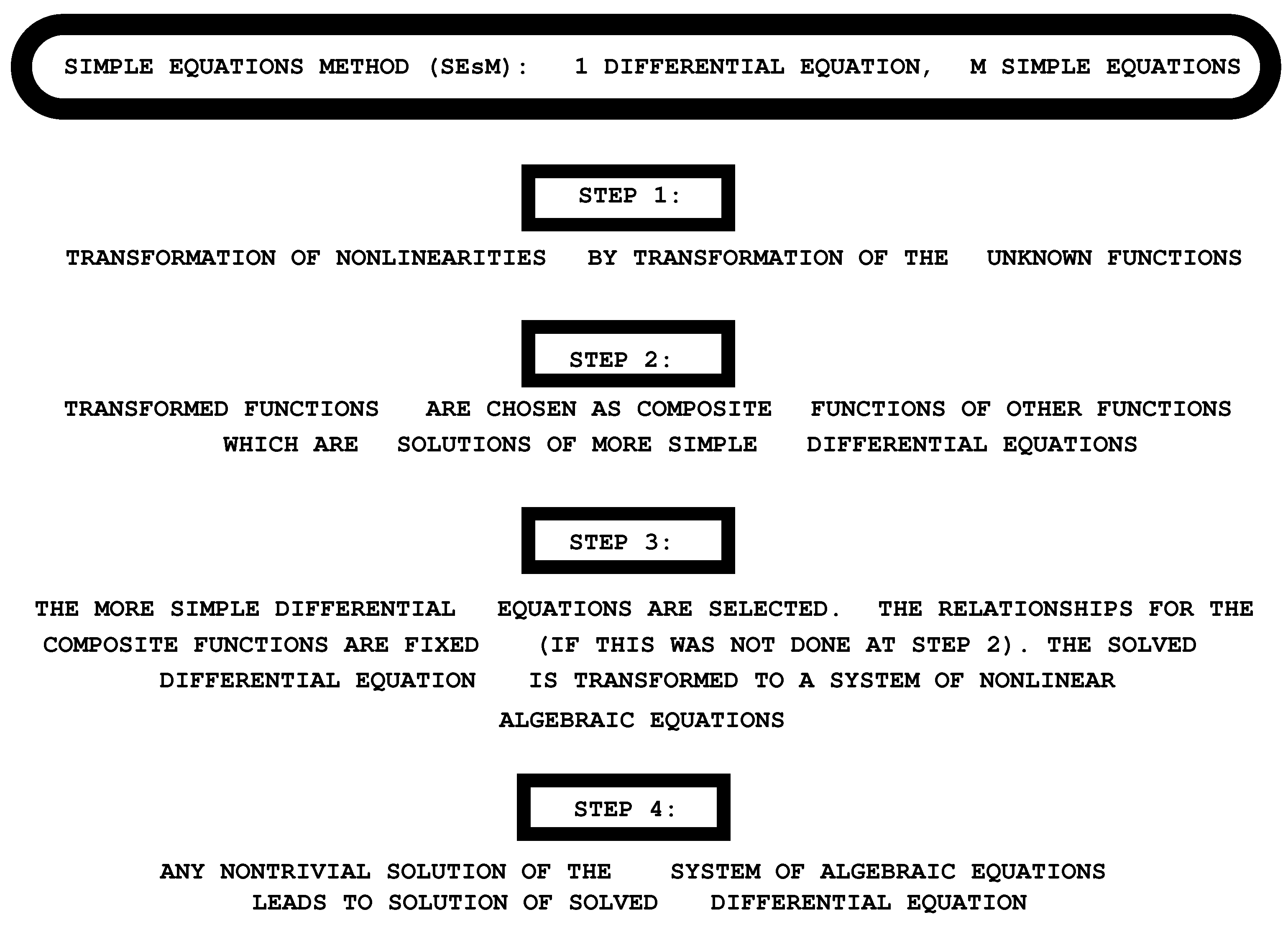
Figure 1.
The Simple Equations Method (SEsM) for the specific case of one solved equation by use of M simple equations. The method has four steps which are described in the text. The discussion in the text below is about the kinds of possible transformations used in Step (1.) of SEsM.
Figure 1.
The Simple Equations Method (SEsM) for the specific case of one solved equation by use of M simple equations. The method has four steps which are described in the text. The discussion in the text below is about the kinds of possible transformations used in Step (1.) of SEsM.

Figure 2.
Examples of a kink and anti-kink described by the solution (14). The parameters are as follows: . , , , , , , . for (a); for (b).
Figure 2.
Examples of a kink and anti-kink described by the solution (14). The parameters are as follows: . , , , , , , . for (a); for (b).

Publisher’s Note: MDPI stays neutral with regard to jurisdictional claims in published maps and institutional affiliations. |
© 2021 by the authors. Licensee MDPI, Basel, Switzerland. This article is an open access article distributed under the terms and conditions of the Creative Commons Attribution (CC BY) license (https://creativecommons.org/licenses/by/4.0/).
Share and Cite
MDPI and ACS Style
Vitanov, N.K.; Dimitrova, Z.I. Simple Equations Method and Non-Linear Differential Equations with Non-Polynomial Non-Linearity. Entropy 2021, 23, 1624. https://0-doi-org.brum.beds.ac.uk/10.3390/e23121624
AMA Style
Vitanov NK, Dimitrova ZI. Simple Equations Method and Non-Linear Differential Equations with Non-Polynomial Non-Linearity. Entropy. 2021; 23(12):1624. https://0-doi-org.brum.beds.ac.uk/10.3390/e23121624
Chicago/Turabian StyleVitanov, Nikolay K., and Zlatinka I. Dimitrova. 2021. "Simple Equations Method and Non-Linear Differential Equations with Non-Polynomial Non-Linearity" Entropy 23, no. 12: 1624. https://0-doi-org.brum.beds.ac.uk/10.3390/e23121624
Note that from the first issue of 2016, this journal uses article numbers instead of page numbers. See further details here.