
Intuitionistic Fuzzy Synthetic Measure on the Basis of Survey Responses and Aggregated Ordinal Data


1
Department of Econometrics and Computer Science, Wroclaw University of Economics and Business, 53-345 Wrocław, Poland
2
Faculty of Computer Science, Bialystok University of Technology, Wiejska 45A, 15-351 Bialystok, Poland
3
Department of Quality and Environmental Management, Wroclaw University of Economics and Business, 53-345 Wrocław, Poland
*
Author to whom correspondence should be addressed.
Entropy 2021, 23(12), 1636; https://0-doi-org.brum.beds.ac.uk/10.3390/e23121636
Submission received: 2 November 2021
/
Revised: 26 November 2021
/
Accepted: 4 December 2021
/
Published: 6 December 2021
(This article belongs to the Special Issue Statistical Methods for Complex Systems)
Abstract
:The paper addresses the problem of complex socio-economic phenomena assessment using questionnaire surveys. The data are represented on an ordinal scale; the object assessments may contain positive, negative, no answers, a “difficult to say” or “no opinion” answers. The general framework for Intuitionistic Fuzzy Synthetic Measure (IFSM) based on distances to the pattern object (ideal solution) is used to analyze the survey data. First, Euclidean and Hamming distances are applied in the procedure. Second, two pattern object constructions are proposed in the procedure: one based on maximum values from the survey data, and the second on maximum intuitionistic values. Third, the method for criteria comparison with the Intuitionistic Fuzzy Synthetic Measure is presented. Finally, a case study solving the problem of rank-ordering of the cities in terms of satisfaction from local public administration obtained using different variants of the proposed method is discussed. Additionally, the comparative analysis results using the Intuitionistic Fuzzy Synthetic Measure and the Intuitionistic Fuzzy TOPSIS (IFT) framework are presented.
1. Introduction
Multiple criteria decision making (MCDM) has been an important research discipline of decision science applied in many areas such as business, management, engineering, and social science [1,2,3]. Nowadays, a lot of new MCDM methods have been introduced to address several practical problems and real-life applications. MCDA methods are widely used in constructing synthetic measures (or composite indicators) for the evaluation of complex socio-economic phenomena [4,5,6].
One of the problems is the assessment of complex socio-economic phenomena using questionnaire surveys when data are represented on an ordinal scale, especially if the object assessments contain positive, negative opinions and an element of uncertainty expressed in the form of no answer, “difficult to say” answer, “no opinion”, etc. In previous studies, some proposals of TOPSIS and Hellwig’s methods based on intuitionistic fuzzy numbers to solve the presented problems were discussed.
The classical Hellwig’s method was presented in 1968 by a Polish researcher as a taxonomic method for international comparison of economic development of countries [7]. This method allows ranking multidimensional objects in terms of a complex phenomenon that cannot be described using a single criterion. The method is based on the concept of distance from the pattern object, which was also used in the well-known and popular TOPSIS method. The difference between both methods is that TOPSIS, apart from the distance from the pattern object, also takes into account the distance from the anti-pattern object.
The methods based on Hellwig’s and TOPSIS methodology have many features in common, whereas the main difference concerns the method for calculating the synthetic variable value. The methods are characterized by the simplicity of calculations and software options (e.g., available free R packages). Both methods allow including quantitative and qualitative criteria in the assessment of objects. In the case of quantitative criteria, their normalization is required. Fuzzy modifications of both methods were proposed for the qualitative criteria. They consist in replacing the qualitative criteria values with fuzzy sets (most frequently fuzzy numbers). In the vast majority of cases the parameters of fuzzy numbers are determined subjectively by the researchers, which does not always allow reflecting the respondents’ preferences in this matter. It is also worth noting that both methods do not suggest how to determine the weighting factors for the criteria. In addition, they do not take into account the potential correlations between the criteria.
Hellwig’s method was promoted in the world literature through the UNESCO research project on the human resources indicators for less developed countries [8,9]. Another application of this method can be found, e.g., in the studies [10,11,12,13,14]. Hellwig’s method was also extended for the fuzzy environment [15,16,17], the intuitionistic fuzzy environment [18,19,20] and the interval-valued intuitionistic fuzzy environment [21].
The idea of using MCDM methods in measuring complex phenomena based on survey data is quite new, therefore the source literature offers only a few scientific publications and research studies addressing this area. The paper [18] presents the concept of the IFSM using Hellwig’s approach for the intuitionistic fuzzy sets. The IFSM allows measuring complex phenomena based on the respondents’ opinions. The IFSM adopts that the respondents assess objects in terms of the adopted criteria using ordinal measurement scales. The respondents’ opinion measurement results are later transformed into intuitionistic fuzzy sets. In another paper [21] a synthetic measure based on Hellwig’s approach and the interval-valued intuitionistic fuzzy set theory is presented. Also, the optimism coefficient is defined, which allows setting the limits of intervals for the proposed parameters. The common feature of both methods is using the transformation of ordinal data to the form of intuitionistic fuzzy sets. The assessment criteria are thus expressed in the form of three parameters of the intuitionistic fuzzy set: membership, non-membership and uncertainty. The difference in these methods consists in determining values of these parameters. In the first case (IFSM method) they are presented as numbers in the interval [0, 1], while in the second case (I-VIFSM method) they take the form of intervals. Finally, [19] proposed the Intuitionistic Fuzzy TOPSIS (IF-TOPSIS) method which can be applied for assessing socio-economic phenomena on the basis of survey data.
Motivated by the above-mentioned works, the present paper proposes the general framework for intuitionistic fuzzy multi-criteria procedure, namely the Intuitionistic Fuzzy Synthetic Measure (IFSM) based on distance to the pattern object. The IFSM method has been inspired by Hellwig’s approach of developing a coefficient adapted to an intuitionistic fuzzy environment.
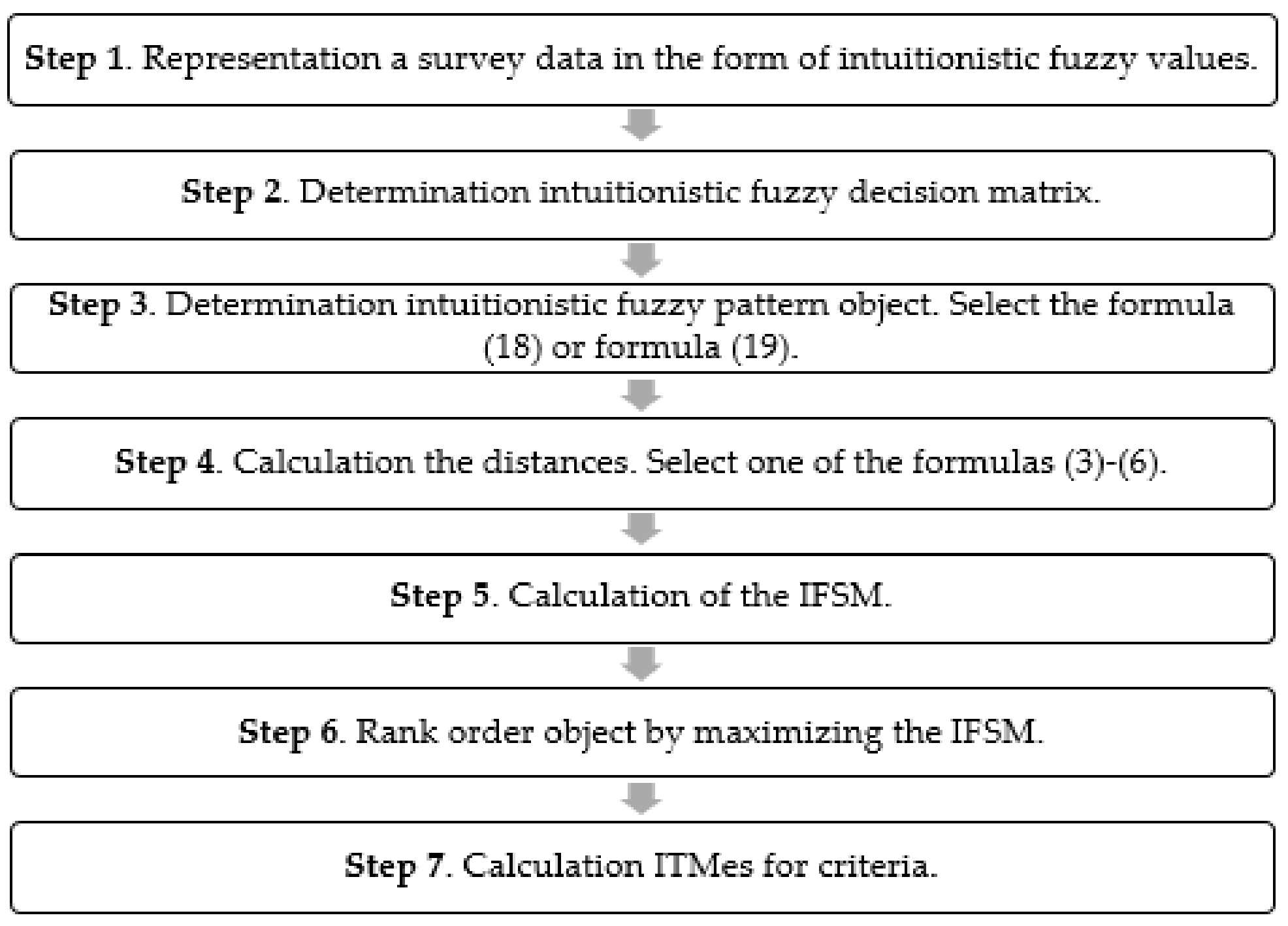
The Intuitionistic Fuzzy Synthetic Measure was proposed to address the problem of survey data. It consists of seven main steps: (1) representation of the survey data in the form of intuitionistic fuzzy values; (2) determination of the Intuitionistic Fuzzy Decision Matrix; (3) determination of the intuitionistic fuzzy pattern object; (4) calculation of the distance measures; (5) calculation of the intuitionistic fuzzy coefficient; (6) rank ordering of objects by maximizing the coefficient; and (7) comparing the criteria with the Intuitionistic Fuzzy Synthetic Measure.
Two concepts for determining intuitionistic fuzzy pattern objects are discussed. The first one is based on max values from the survey data and the second on max intuitionistic values in general. Next, two measures of distances, i.e., Euclidean and Hamming distance implemented in the coefficient procedure are considered which, additionally, can be based on two or three parameters. This provides eight variants of the proposed IFSM. The usefulness of the proposed approach was examined in the evaluation of satisfaction from local public administration in the context of quality of life in cities using survey data.
As was pointed out by [22] the purpose of constructing synthetic measure, among other things, “to condense and summarise the information contained in a number of underlying indicators, in a way that accurately reflects the underlying concept”. Thus finally, the Spearman coefficient for comparison criteria with respect to information transferred for the IFSM is proposed.
The objectives and contributions of this study are presented below:
- to develop a general IFSM based on Hellwig’s approach for the evaluation of socio-economic phenomena with survey data;
- to study the IFSM based on Hellwig’s approach taking into account two types of Euclidean and Hamming distance implemented in the procedure;
- to study the IFSM based on Hellwig’s approach considering two or three parameters used in distance measure applied in the procedure;
- to study the IFSM based on Hellwig’s approach examining different pattern object construction used in the procedure;
- to propose the method for criteria comparison with the Intuitionistic Fuzzy Synthetic Measure;
- to demonstrate different variants of the Intuitionistic Synthetic Measure based on Hellwig’s approach through a comparative analysis;
- to compare different variants of the IFSM based on Hellwig’s approach with the Intuitionistic Fuzzy TOPSIS (IFT) procedure to examine its relevance and effectiveness.
The proposed framework, based on the extended Hellwig’s method, has been applied to analyse its relevance.
The rest of this article is organized as follows. In Section 2 the basic concepts related to intuitionistic fuzzy sets (IFS) and distances on IFSs are presented. The general framework of the IFSM based on Hellwig’s approach is provided in Section 3. Section 4 discusses a case study solving the problem of rank-ordering of the cities in terms of satisfaction from local public administration using the proposed approach. The comparison results obtained using the IFSM with the IFT framework are also presented. The conclusion and indications for future research are formulated in Section 4.
2. Preliminaries
To start with, the presentation of some basic concepts related to IFS and distances on IFSs are presented.
The Intuitionistic Fuzzy Set theory, proposed by Atanassov [23], is an extension of the Fuzzy Set (FS) theory introduced by Zadeh [24] to address uncertainty.
Definition 1
The numbers and denote, respectively, the degrees of membership and non-membership of the element to the set ; the intuitionistic fuzzy index (hesitation margin) of the element in the set . Greater indicates more vagueness. It should be noticed that when for every then intuitionistic fuzzy set is an ordinary fuzzy set.
If the universe contains only one element , then the IFS over is denoted as and called an intuitionistic fuzzy value (IFV) [26,27]. Let be the set of all IFVs. The intuitionistic value is the largest, while is the smallest.
One of the applications of intuitionistic fuzzy sets in multiple criteria decision making is the possibility of taking into consideration the decision maker’s approval, rejection, and hesitations regarding the evaluated alternatives with respect to criteria. This is the main motivation for using the intuitionistic fuzzy sets in developing the multi-criteria procedure.
Euclidean and Hamming distances represent the widely used distances for the intuitionistic fuzzy sets [28].
Definition 2
([28]). Let us consider two with membership functions , , and non-membership functions , , respectively. The normalized Euclidean between two intuitionistic fuzzy sets A and B is defined as:
The normalized Hamming distance between two intuitionistic fuzzy sets A and B is defined as:
To compare two IFVs the following score function defined by Chen & Tan [29] was used:
and accuracy function defined by Hong and Choi [30]:
It can be easily observed that and .
Definition 3
- 1.
- if , then ;
- 2.
- if , and
- (i)
- , then ;
- (ii)
- , then .
3. Classical and Intuitionistic Variant of Hellwig’s Method
3.1. Classical Variant of Hellwig’s Method
The classical Hellwig’s method was proposed for quantitative criteria. It adopts the calculation of Euclidean distance from the pattern of development for each assessed object. Most often the pattern of development is an abstract unit presenting the most favorable assessments of the individual criteria. Let be the set of objects subject to assessment and the set of criteria constituting a complex phenomenon. It should also be adopted that and are the sets of stimulating (positive) and destimulating (negative) criteria, respectively, influencing the complex phenomenon . The classical variant of Hellwig’s method consists of the following steps:
Step 1. Defining the decision matrix:
where is the value of the -th object with respect to the -th criterion.
Step 2. Determining the normalized decision matrix:
using the formula for standardization:
where: , .
Step 3. Defining the pattern of development (pattern object) in accordance with the principle:
Step 4. Calculating the distance of the -th object from the pattern of development using the Euclidean distance:
Step 5. Calculating the synthetic measure of development for the -th object:
where: , , .
Step 6. Ranking the objects according to the decreasing values of .
The measure most often takes values from the interval . The higher values of the measure the less the object is away from the pattern of development.
3.2. The Intuitionistic Fuzzy Synthetic Measure Based on Hellwig’s Approach for the Evaluation of Socio-Economic Phenomena Using Survey Data
In this section, a general framework for Intuitionistic Fuzzy Synthetic Measures is proposed. Let be the set of objects under the survey evaluation, the set of criteria for the objects assessed by the respondents using an ordinal measurement scale. The respondents’ answers are collected in a questionnaire survey. It was adopted that the respondents answered the questions using different scales, which can be aggregated into three groups: “a positive opinion about the object”, “a negative opinion about the object”, “no opinion or no answer”. The same importance was adopted in the evaluation of objects to the criteria. i.e., the weights of criteria are equal [32].
The procedure to evaluate the socio-economic phenomena is as follows:
Step 1. Representation of the survey data in the form of intuitionistic fuzzy values.
The respondents’ opinions about the object for each criterion are represented by IFVs , where:
- —the fraction of positive opinions about i-th object with respect to j-th criterion,
- —the fraction of negative opinions about i-th object with respect to j-th criterion,
- —the fraction of opinion type “don’t know”, “no answers” for i-th object with respect to j-th criterion, and .
The following has been adopted:
where:
- —the total number of respondents who positively evaluated the i-th object with respect to j-th criterion;
- —the total number of respondents who negatively evaluated the i-th object with respect to j-th criterion;
- —the total number of respondents with hesitancy opinion about the i-th object for j-th criterion;
- —the total number of respondents who evaluated the i-th object with respect to the j-th criterion.
It has been noted that .
Clearly, instead of the total number of responses, the percentage of relevant responses common for the secondary survey data can be used.
In this way i-th object is represented by the vector:
where .
Step 2. Determination of the Intuitionistic Fuzzy Decision Matrix.
Based on the survey data representation in the form of intuitionistic fuzzy values obtained in step 1 the intuitionistic fuzzy decision matrix is given in the form:
Step 3. Determination of the intuitionistic fuzzy pattern object.
The intuitionistic fuzzy pattern object can be determined twofold:
- is based on maximum IFV and takes the form of:
- is based on maximum and minimum values and takes the form of:where , denote the evaluation information of i-th object with respect to j-th criterion and .
Step 4. Calculation of the distance measures.
After selecting the distance measure, the distance measures between the objects and the intuitionistic fuzzy pattern object selected in step 3 are calculated using one of the Formulas (3)–(6).
The distance measure from the pattern object takes the form of:
where , .
Step 5. Calculation of the Intuitionistic Fuzzy Synthetic Measure.
The Intuitionistic Fuzzy Synthetic Measure (IFSM) coefficient is defined as follows:
where: , , .
Step 6. Rank ordering of objects by maximizing the coefficient .
The highest value of then the highest position of the object .
Step 7. Comparing the individual criteria with the Intuitionistic Fuzzy Synthetic Measure using Information Transfer Measure (ITM).
The important two problems should be addressed while building the IFSM, condensing information and accurately representing the underlying concept. The criteria should capture the most important properties of the analyzed phenomena, represent them accurately and provide a large amount of information. There should be a positive correlation between the criteria and the synthetic measure, and also each criterion should contribute to the decision-maker(s)’ views on its importance regarding the concept [22]. Now the measure of the information transferred from each criterion to the IFSM is defined. The criteria should capture the most important properties of the analyzed phenomena, represent them accurately and provide a large amount of information.
First, the individual criteria represented by the intuitionistic fuzzy values are ordered using accuracy function and score function (see Definition 3). Then the Spearman coefficient between the ranking criteria and the ranking obtained by the IFSM measure is calculated. The Spearman coefficient is a nonparametric measure of dependence for the variables measured at least on an ordinal scale. The measure is normalized in the range [–1, 1]. It allows measuring the power and determining the direction of the correlations. Formally, the Information Transfer Measure for j-th criterion is defined as follows:
The shows the power and direction between the criterion and the synthetic measure . It should be observed that taking into account the way of survey data representation in the form of intuitionistic fuzzy values this coefficient should be positive. In the case where the importance of the criterion is the same, the measures for should be similar.
The procedure of analyzing the survey data for IFSM is presented in Figure 1.
Classification of variants of the IFSM based on an intuitionistic fuzzy framework with respect to pattern objects and distance measures is presented in Table 1.
4. Empirical Example
4.1. Problem Description and Data Source
The approach to the analysis of survey data proposed in the article, applying the presented procedure and the IFSM method, was used in the analysis of the results from the fifth survey on quality of life in European cities. The survey provides a unique insight into city life. It gathers the experience and opinions of city dwellers.
The fifth survey on quality of life in European cities was conducted for the European Commission by the IPSOS company. The survey covered the inhabitants of 83 cities in the EU, the EFTA countries, the UK, the Western Balkans, and Turkey. The survey was conducted between 12 June and 27 September 2019, with a break between 15 July and 1 September. A total of 700 interviews were completed in each surveyed city. This means that a total of 58,100 inhabitants of 83 cities participated in the survey.
The survey covers eight fields of the quality of life in cities: overall satisfaction, services and amenities, environmental quality, economic well-being, public transport, the inclusive city, local public administration, as well as safety and crime. For the first time, the fifth round of the survey includes questions about the quality of the city administration. The high-quality, efficient, and transparent local public administration is very important for improving the quality of life in European cities. In addition, improving the quality of institutions at the local level is the heart of the EU and the EU Cohesion Policy. In the empirical example, European cities would be ranked only in the field of local public administration. Thus, only five questions of the questionnaire concerning satisfaction from the local public administration were used [33]:
“I will read you a few statements about the local public administration in your city. Please tell me whether you strongly disagree, somewhat disagree,…
Q1: I am satisfied with the amount of time it takes to get a request solved by my local public administration;
Q2: The procedures used by my local public administration are straightforward to understand;
Q3: The fees charged by my local public administration are reasonable;
Q4: Information and services of my local public administration can be easily accessed online;
Q5: There is corruption in my local public administration.”
Our study aims at measuring and benchmarking inhabitants’ satisfaction with local public administration using the IFSM approach. Inhabitants’ satisfaction, as a complex phenomenon, was characterized using five criteria described by five questions Q1–Q5: C1—time for request, C2—procedures; C3—fees charged, C4—information and services, C5—corruption. In the assessment of criteria, a five-point measurement scale was used: strongly disagree, somewhat disagree, somewhat agree, strongly agree, don’t know/no answer.
The characteristics of the research sample in terms of gender, age, and level of education are presented in Table 2.
4.2. Analysis of the Results
In this part, the empirical results concerning the evaluation of the satisfaction with local public administration in European cities using the IFSMes are presented. Due to the large number of cities covered by the survey individual steps of the proposed procedure were presented based on the example of the selected 2 cities: Zurich (the best in all rankings) and Palermo (the worst in all rankings). The selected cities were the first and the last in the ranking obtained using all IFSM methods. The assessment of the selected cities in terms of 5 criteria using the 5 categories is presented in Table 3.
According to Formula (15), the respondents’ assessments were transformed into IFVs (Table 4).
It has been observed that for the criteria C1, C2, C3, C4 the is obtained by summing up the categories 1, 2, and by summing up the categories 3, 4. Taking into account the form of question Q5 for the criterion C5 the value is obtained by summing up the categories 3, 4 while by summing up the categories 1, 2. The assessment criteria in the form of IFVs for all cities are listed in Table A1, Table A2 and Table A3 in the Appendix A.
The assessments of cities in terms of five criteria in the form of IFVs were used to construct an intuitionistic fuzzy decision matrix, a fragment of which is presented below for the three selected cities:
Weights have not been assigned to individual criteria. In our opinion, all the aspects (e.g., time for request, procedures, fees charged, information and services, corruption) should be balanced, i.e., they are equally important in evaluating satisfaction from the local administration.
The coordinates of intuitionistic fuzzy pattern objects were determined twofold: based on (1,0) values and second for maximum and minimum IFVs, respectively (Table 5 and Table 6).
Using the normalized Euclidean or Hamming distance in accordance with the Formulas (3)–(6) the distances of each city from the intuitionistic fuzzy pattern objects and values were calculated. Finally, the IFSM coefficients were calculated (Table 7).
The values of IFSM coefficients for all cities are presented in Table A4 in the Appendix A.
The position of cities in the ranking was determined based on the IFSM coefficient values, following the principle that the higher the value of the IFSM coefficient, the higher the city’s position in the ranking (Table A5; Appendix A).
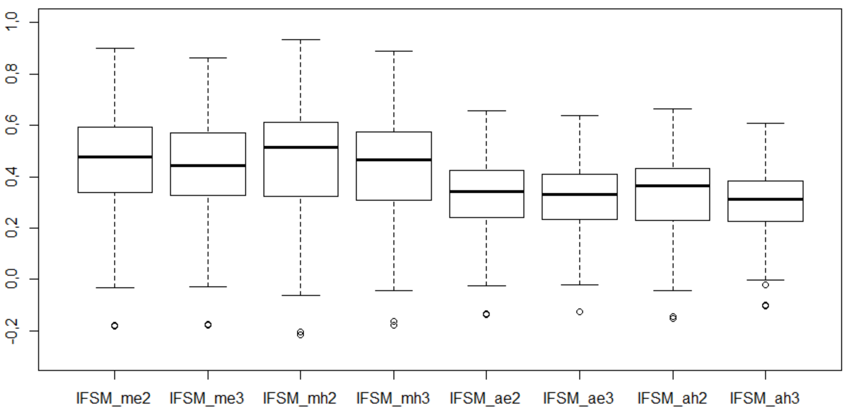
Descriptive statistics and box plots for the values of IFSM coefficients are presented in Table 8 and Figure 2.
- determining the coordinates of the pattern object based on intuitionistic values (1,0) resulted in a lower value of the IFSM for cities compared with the IFSM when the coordinates of the pattern object are based on max and min values. The IFSM area of variability also decreased;
- the IFSM similarly differentiates cities in terms of the adopted synthetic criterion, i.e., satisfaction with public administration services; regardless of the method used for determining the coordinates of the pattern object, the number of cities for which the IFS values are below and above the IFSM average remains at a similar level;
- regardless of the method for determining the coordinates of the pattern object, the IFSM values present a slight response to the choice of the distance measure and the number of parameters that take these distances into account. The introduction of the third uncertainty parameter in measuring the distance between cities and the pattern object slightly lowers the mean values of IFSM and reduces the variability range of these values. This regularity has been observed for two methods used in determining the coordinates of the pattern object.
The Spearman coefficients between IFSM values are presented in Table 9.
The choice between the Euclidean and Hamming distance and the method for determining the coordinates of the pattern objects does not have a large impact on the ranking positions of the cities. High values of the Spearman coefficient suggest slight changes in the ranking position of the cities. If the Hamming distance for two parameters is used in IFSM, the choice of the method for determining the coordinates of the pattern objects is irrelevant. In both cases, the value of the Spearman coefficient was equal to one, which means the same ranking of the cities in terms of satisfaction with public administration services. The lowest similarity of rankings (Spearman coefficient value equal to 0.870) was observed for the IFSM with the Hamming distance with two and three parameters, respectively, for the coordinates of the pattern objects determined based on the values (max, min) and (1,0).
The Information Transfer Measures for the IFSMes are presented in Table 10.
The criteria are well represented by the IFSM. The largest information transfer occurred for C1 criterion (regardless of the IFSM variant). The smallest information transfer was recorded for C3 criterion. All the criteria are the least represented by the IFSM_ae3 variant. The same values of Spearman coefficients were observed for the two variants: IFSM_mh2 and IFSM_ah2. This result is not surprising since equal rankings were obtained using these variants of the methods (see Table 10).
4.3. Comparative Analysis and Implications
Hellwig’s method uses only the concept of a positive pattern object (named as the pattern of development), while the well known TOPSIS method [34] used the concept of pattern and anti-pattern object (ideal and anty-ideal solution, respectively). The TOPSIS with many modifications in the fuzzy and intuitionistic fuzzy environment has been proposed and applied in real-life problems [19,35,36].
Similarly, a description of variants of the IFTes with respect to pattern objects and distance measures used in comparative analysis is presented in Table 11 (for details see [19]).
The coordinates of an intuitionistic fuzzy anti-pattern object based on (0,1) values or max and min in the IFT are presented in Table 12. The coordinates of an intuitionistic fuzzy anti-pattern object based on max and min values are presented in Table 13.
Descriptive statistics and box plots for the values of IFT coefficients are presented in Table 14 and Figure 3.
Determining the coordinates of the pattern object based on the values (max, min) resulted in the average IFT values presenting a very similar level with a highly corresponding variability range. In this case, choosing the distance measure and taking into account the degree of uncertainty in its measurement are of no great importance.
Establishing the coordinates of the pattern object based on the intuitionistic values (1,0) significantly reduced the variability range of the IFT values. Moreover, for this type of pattern object, the IFT has become more sensitive to the number of parameters included in measuring the distance between cities and the pattern object. It is evident that the average IFT values increased after taking into account the degree of uncertainty for both the Euclidean and Hamming distances. The variability range of IFT values, in this case, is also the smallest among all the analyzed IFT variants.
The Spearman coefficients between IFT measures are presented in Table 15.
The total consistency of the city rankings using the IFT (Spearman coefficient value equal to 1) was obtained for the Hamming distance with two parameters and for the coordinates of pattern objects determined based on the values (max, min) and (1,0), respectively. However, the lowest still very high consistency of rankings was found in two cases. In the first one, the IFT values were calculated by defining the pattern object coordinates based on the value (1,0) and using the Hamming distance for 2 and 3 parameters, respectively. The second case was very similar and the difference was only in the method used for determining the pattern object coordinates.
The Information Transfer Measures for the IFTes are presented in Table 16.
All the criteria are very well represented by the IFT. It is not possible to identify the IFT variant following which the information transfer for all the criteria is the highest or the lowest. As with the IFSM, an identical information transfer for each criterion was observed for IFT_mh2 and IFT_ah2. Regardless of the IFT variant, C3 was the least represented, whereas C1 received the strongest representation of all the criteria applied.
Spearman coefficients between the IFSM and the IFT measures are presented in Table 17.
The compared measures, regardless of the distance used and the coordinates of the pattern object, rank cities in a very similar way in terms of satisfaction with public administration services. The lowest value of the Spearman coefficient was 0.971, which means very high consistency of all the obtained rankings. In the case of using the pattern object, the coordinates of which were determined based on intuitionistic values (1,0), and the Hamming distance, it did not matter whether the IFSM or the IFT measure was used in ranking the cities (Spearman coefficient value was 1). In this case, it was also irrelevant to include the uncertainty parameter in the calculation of the distance between the cities and the pattern city.
Identical results of the city rankings using the IFSM, and the IFT were also recorded for the combination of the Hamming measure with two parameters and the coordinates of the pattern objects determined based on max and min values. Taking into account the uncertainty parameter in this case resulted in slight changes in the ranking position of some cities.
5. Conclusions
The paper proposes the IFSM as a method for measuring complex phenomena based on survey data. Most frequently, this type of data takes the form of ordinal data. In this case the measurement results at the level of individual respondents are not required. The suggested method allows measuring complex phenomena from aggregated ordinal data offered by public statistics. The proposed approach adopts the transformation of aggregated ordinal data into intuitionistic fuzzy sets. The IFSM construction, as with other synthetic measures, requires the researcher to make subjective decisions regarding, e.g., the choice of the distance measure and how to determine the coordinates of the pattern object. Therefore, this paper provides a comparative analysis addressing the two most popular distances for the intuitionistic fuzzy sets, the Euclidean distance and the Hamming distance. Both two and three parameters of the intuitionistic fuzzy sets were taken into account in the distance calculation. The construction of a pattern object based on the intuitionistic values was also proposed and compared with the classical approach, where the coordinates of the pattern object are determined based on the maximum and minimum criterion assessments observed in the research sample. In addition, the findings collected using the IFSM were compared with the IFT since both methods are very similar in their construction and use the idea of pattern (reference) objects.
The empirical example presented in the paper as well as the comparative analyses carried out for different variants of the IFSM method allowed formulating the following conclusions:
- in each of the eight analyzed variants of the synthetic measure construction, the mean values of IFT for the cities were higher than in the case of IFSM. Furthermore, in each of these cases the variability range of IFT values was lower than that of IFSM. This is primarily true when the coordinates of the pattern objects were established based on the intuitionistic values (1,0);
- in the case of the pattern object coordinates determined based on the values (max, min), very similar changes in the ranges of their value variability were observed for the IFSM and IFT, depending on the selected distance measure and the number of parameters included in it;
- determining the coordinates of the pattern objects based on the value (1,0) caused that the values of IFSM and IFT changed in an opposite way as a result of the applied distance and taking into account the degree of uncertainty. The increase in the value of the IFT measure for the cities occurred along with the decrease in the value of IFSM and vice versa. It should be noted, however, that the increase in IFT values took place at a reduced variability range. In the case of IFSM such a large reduction in variability was not observed. Therefore, the application of the IFSM in the variant with the pattern object, the coordinates of which are determined based on the intuitionistic values (1,0), allowed for differentiating cities to a greater extent in terms of the complex phenomenon, i.e., satisfaction with public administration services;
- for the analyzed data set, the ranking of cities determined on the basis of both IFSM and IFT values turned out to be a little sensitive to the choice of the distance measure and the method for determining the coordinates of pattern objects. The values of the correlation coefficients for the obtained rankings were very high, reaching the value of 1 in some cases. Slightly greater consistency of the rankings was obtained for the IFT, which suggests a somewhat higher sensitivity of the IFSM to the choice of the distance measure and the method for determining the coordinates of the pattern object. In the case of both methods, the highest ranking consistency was recorded using the Hamming distance for two parameters and the coordinates of pattern objects established based on the values (max, min) and (1,0), respectively. Therefore, including the third parameter in measuring the distance, taking the form of the degree of uncertainty, changes the position of cities in the rankings, although in the presented example these changes were small and referred to some cities only. The least consistent rankings for both measures were also observed for the Hamming distance, however, for a different number of parameters combined with:
- (a)
- pattern objects, the coordinates of which were determined based on the values (1,0);
- (b)
- pattern objects, the coordinates of which were determined based on the values (1,0) and (max, min).
It should be highlighted that, despite the high consistency of the obtained rankings, the values of measures for cities were diversified, which suggests a different level of residents’ satisfaction with public administration services. It is of particular importance in the context of monitoring the analyzed phenomenon over time because the same position of a city in the ranking does not imply that the level of the phenomenon is not going to increase over time; - it is difficult to identify, from among the IFSM and the IFT, a better method in terms of representing the particular criteria. All criteria are very well represented by both the IFSM and the IFT. In either case, the largest transfer of information was recorded for C1 and the smallest for C3.
A certain limitation of the proposed method for transforming ordinal data is that there is no possibility to differentiate categories on the side of “positive” and “negative” responses. This may have an impact on the synthetic measure values and the ranking positions of the assessed objects. One of the directions for further research on the IFSM will be presenting some proposals in this area. The influence of data distribution on the results of object ranking using the IFSM will also be analyzed.
Author Contributions
Conceptualization, E.R., M.K.-J. and B.J.; methodology, E.R., M.K.-J. and B.J.; validation, E.R., M.K.-J. and B.J., formal analysis, E.R., M.K.-J. and B.J.; investigation, E.R., M.K.-J. and B.J.; resources, E.R., M.K.-J. and B.J.; data curation, E.R., M.K.-J. and B.J.; writing—original draft preparation, E.R., M.K.-J. and B.J.; writing—review and editing, E.R., M.K.-J. and B.J.; visualization, M.K.-J. and B.J.; supervision, E.R.; administration, E.R. All authors have read and agreed to the published version of the manuscript.
Funding
This research received no external funding.
Institutional Review Board Statement
Not applicable.
Informed Consent Statement
Not applicable.
Data Availability Statement
Not applicable (for secondary data analysis, see [33]).
Conflicts of Interest
The authors declare no conflict of interest.
Appendix A

Table A1.
Degrees of non-membership to IFVs for cities.
| City | C1 | C2 | C3 | C4 | C5 |
|---|---|---|---|---|---|
| Aalborg | 0.164 | 0.293 | 0.246 | 0.101 | 0.166 |
| Amsterdam | 0.327 | 0.367 | 0.413 | 0.127 | 0.281 |
| Ankara | 0.409 | 0.335 | 0.425 | 0.242 | 0.422 |
| Antalya | 0.349 | 0.213 | 0.344 | 0.134 | 0.337 |
| Antwerpen | 0.260 | 0.199 | 0.371 | 0.358 | 0.264 |
| Athina | 0.619 | 0.580 | 0.724 | 0.352 | 0.584 |
| Barcelona | 0.540 | 0.353 | 0.582 | 0.302 | 0.435 |
| Belfast | 0.307 | 0.302 | 0.323 | 0.156 | 0.370 |
| Beograd | 0.624 | 0.617 | 0.558 | 0.280 | 0.749 |
| Berlin | 0.579 | 0.600 | 0.293 | 0.269 | 0.371 |
| Białystok | 0.290 | 0.348 | 0.292 | 0.127 | 0.301 |
| Bologna | 0.442 | 0.459 | 0.487 | 0.192 | 0.386 |
| Bordeaux | 0.382 | 0.357 | 0.321 | 0.217 | 0.265 |
| Braga | 0.456 | 0.303 | 0.402 | 0.250 | 0.535 |
| Bratislava | 0.333 | 0.465 | 0.267 | 0.247 | 0.498 |
| Bruxelles | 0.363 | 0.211 | 0.344 | 0.248 | 0.284 |
| Bucharest | 0.458 | 0.490 | 0.321 | 0.280 | 0.639 |
| Budapest | 0.395 | 0.337 | 0.376 | 0.131 | 0.373 |
| Burgas | 0.439 | 0.392 | 0.476 | 0.141 | 0.535 |
| Cardiff | 0.238 | 0.269 | 0.295 | 0.139 | 0.196 |
| Cluj-Napoca | 0.279 | 0.316 | 0.249 | 0.179 | 0.580 |
| Diyarbakir | 0.572 | 0.494 | 0.381 | 0.394 | 0.507 |
| Dortmund | 0.460 | 0.527 | 0.450 | 0.248 | 0.396 |
| Dublin | 0.284 | 0.249 | 0.264 | 0.132 | 0.339 |
| Essen | 0.368 | 0.530 | 0.323 | 0.212 | 0.236 |
| Gdańsk | 0.316 | 0.344 | 0.280 | 0.155 | 0.356 |
| Genève | 0.159 | 0.200 | 0.362 | 0.232 | 0.384 |
| Glasgow | 0.381 | 0.318 | 0.368 | 0.172 | 0.330 |
| Graz | 0.316 | 0.254 | 0.277 | 0.108 | 0.225 |
| Groningen | 0.188 | 0.199 | 0.407 | 0.080 | 0.167 |
| Hamburg | 0.302 | 0.449 | 0.300 | 0.196 | 0.251 |
| Helsinki | 0.373 | 0.505 | 0.297 | 0.218 | 0.341 |
| Irakleio | 0.651 | 0.548 | 0.716 | 0.193 | 0.627 |
| Istanbul | 0.463 | 0.331 | 0.428 | 0.275 | 0.564 |
| København | 0.299 | 0.323 | 0.206 | 0.100 | 0.167 |
| Košice | 0.346 | 0.357 | 0.284 | 0.173 | 0.481 |
| Kraków | 0.311 | 0.479 | 0.393 | 0.161 | 0.298 |
| Lefkosia | 0.461 | 0.206 | 0.425 | 0.135 | 0.593 |
| Leipzig | 0.256 | 0.329 | 0.367 | 0.157 | 0.203 |
| Liège | 0.309 | 0.220 | 0.360 | 0.228 | 0.312 |
| Lille | 0.434 | 0.332 | 0.385 | 0.279 | 0.255 |
| Lisboa | 0.574 | 0.476 | 0.501 | 0.262 | 0.572 |
| Ljubljana | 0.347 | 0.323 | 0.207 | 0.175 | 0.563 |
| London | 0.374 | 0.340 | 0.342 | 0.144 | 0.259 |
| Luxembourg | 0.262 | 0.289 | 0.209 | 0.147 | 0.310 |
| Madrid | 0.418 | 0.382 | 0.446 | 0.264 | 0.398 |
| Málaga | 0.402 | 0.335 | 0.386 | 0.229 | 0.417 |
| Malmö | 0.334 | 0.464 | 0.235 | 0.173 | 0.252 |
| Manchester | 0.243 | 0.261 | 0.272 | 0.115 | 0.387 |
| Marseille | 0.429 | 0.397 | 0.503 | 0.361 | 0.457 |
| Miskolc | 0.232 | 0.271 | 0.362 | 0.083 | 0.439 |
| Munich | 0.354 | 0.401 | 0.273 | 0.156 | 0.191 |
| Naples | 0.719 | 0.626 | 0.711 | 0.411 | 0.607 |
| Oslo | 0.452 | 0.460 | 0.330 | 0.222 | 0.279 |
| Ostrava | 0.363 | 0.436 | 0.266 | 0.123 | 0.534 |
| Oulu | 0.349 | 0.455 | 0.372 | 0.240 | 0.286 |
| Oviedo | 0.466 | 0.444 | 0.527 | 0.301 | 0.472 |
| Palermo | 0.836 | 0.689 | 0.765 | 0.450 | 0.719 |
| Paris | 0.423 | 0.379 | 0.401 | 0.256 | 0.305 |
| Piatra Neamt | 0.327 | 0.360 | 0.283 | 0.194 | 0.562 |
| Podgorica | 0.515 | 0.427 | 0.317 | 0.310 | 0.670 |
| Praha | 0.396 | 0.439 | 0.190 | 0.149 | 0.471 |
| Rennes | 0.368 | 0.311 | 0.315 | 0.201 | 0.164 |
| Reykjavík | 0.516 | 0.496 | 0.506 | 0.211 | 0.570 |
| Riga | 0.443 | 0.471 | 0.712 | 0.268 | 0.681 |
| Rome | 0.827 | 0.710 | 0.727 | 0.402 | 0.772 |
| Rostock | 0.199 | 0.386 | 0.254 | 0.175 | 0.234 |
| Rotterdam | 0.380 | 0.334 | 0.311 | 0.185 | 0.223 |
| Skopje | 0.675 | 0.437 | 0.423 | 0.328 | 0.764 |
| Sofia | 0.524 | 0.520 | 0.461 | 0.248 | 0.503 |
| Stockholm | 0.368 | 0.427 | 0.217 | 0.174 | 0.225 |
| Strasbourg | 0.322 | 0.304 | 0.359 | 0.246 | 0.252 |
| Tallinn | 0.251 | 0.313 | 0.147 | 0.127 | 0.563 |
| Tirana | 0.482 | 0.396 | 0.510 | 0.229 | 0.756 |
| Turin | 0.642 | 0.611 | 0.648 | 0.299 | 0.492 |
| Tyneside conurbation | 0.280 | 0.263 | 0.331 | 0.177 | 0.270 |
| Valletta | 0.319 | 0.252 | 0.200 | 0.141 | 0.185 |
| Verona | 0.530 | 0.541 | 0.395 | 0.235 | 0.596 |
| Vilnius | 0.393 | 0.342 | 0.385 | 0.251 | 0.423 |
| Warszawa | 0.391 | 0.485 | 0.435 | 0.191 | 0.331 |
| Wien | 0.232 | 0.310 | 0.266 | 0.119 | 0.226 |
| Zagreb | 0.654 | 0.601 | 0.588 | 0.220 | 0.753 |
| Zurich | 0.124 | 0.206 | 0.188 | 0.083 | 0.171 |
Table A2.
Degrees of membership to IFVs for cities.
| City | C1 | C2 | C3 | C4 | C5 |
|---|---|---|---|---|---|
| Aalborg | 0.670 | 0.608 | 0.568 | 0.846 | 0.788 |
| Amsterdam | 0.487 | 0.571 | 0.524 | 0.805 | 0.447 |
| Ankara | 0.562 | 0.642 | 0.562 | 0.725 | 0.492 |
| Antalya | 0.644 | 0.780 | 0.639 | 0.817 | 0.518 |
| Antwerpen | 0.557 | 0.724 | 0.619 | 0.526 | 0.468 |
| Athina | 0.374 | 0.405 | 0.264 | 0.526 | 0.174 |
| Barcelona | 0.446 | 0.628 | 0.408 | 0.668 | 0.481 |
| Belfast | 0.500 | 0.630 | 0.581 | 0.690 | 0.418 |
| Beograd | 0.328 | 0.359 | 0.405 | 0.596 | 0.088 |
| Berlin | 0.326 | 0.315 | 0.602 | 0.553 | 0.293 |
| Białystok | 0.687 | 0.612 | 0.678 | 0.764 | 0.442 |
| Bologna | 0.518 | 0.508 | 0.500 | 0.744 | 0.485 |
| Bordeaux | 0.575 | 0.587 | 0.598 | 0.724 | 0.484 |
| Braga | 0.485 | 0.660 | 0.564 | 0.677 | 0.281 |
| Bratislava | 0.509 | 0.462 | 0.659 | 0.667 | 0.231 |
| Bruxelles | 0.627 | 0.789 | 0.619 | 0.700 | 0.498 |
| Bucharest | 0.458 | 0.491 | 0.637 | 0.552 | 0.118 |
| Budapest | 0.459 | 0.567 | 0.523 | 0.677 | 0.304 |
| Burgas | 0.519 | 0.567 | 0.480 | 0.802 | 0.305 |
| Cardiff | 0.572 | 0.651 | 0.637 | 0.754 | 0.573 |
| Cluj-Napoca | 0.628 | 0.601 | 0.696 | 0.630 | 0.131 |
| Diyarbakir | 0.375 | 0.495 | 0.599 | 0.574 | 0.428 |
| Dortmund | 0.504 | 0.435 | 0.479 | 0.654 | 0.341 |
| Dublin | 0.589 | 0.659 | 0.637 | 0.777 | 0.483 |
| Essen | 0.566 | 0.364 | 0.574 | 0.658 | 0.382 |
| Gdańsk | 0.632 | 0.613 | 0.683 | 0.781 | 0.378 |
| Genève | 0.717 | 0.746 | 0.573 | 0.684 | 0.384 |
| Glasgow | 0.477 | 0.558 | 0.529 | 0.669 | 0.492 |
| Graz | 0.628 | 0.711 | 0.697 | 0.831 | 0.591 |
| Groningen | 0.551 | 0.607 | 0.543 | 0.827 | 0.600 |
| Hamburg | 0.629 | 0.476 | 0.579 | 0.714 | 0.418 |
| Helsinki | 0.391 | 0.398 | 0.609 | 0.723 | 0.598 |
| Irakleio | 0.324 | 0.424 | 0.265 | 0.656 | 0.315 |
| Istanbul | 0.508 | 0.630 | 0.517 | 0.681 | 0.323 |
| København | 0.589 | 0.580 | 0.616 | 0.833 | 0.789 |
| Košice | 0.569 | 0.579 | 0.674 | 0.732 | 0.228 |
| Kraków | 0.593 | 0.478 | 0.564 | 0.746 | 0.369 |
| Lefkosia | 0.531 | 0.771 | 0.534 | 0.736 | 0.362 |
| Leipzig | 0.631 | 0.596 | 0.551 | 0.634 | 0.378 |
| Liège | 0.569 | 0.747 | 0.613 | 0.606 | 0.396 |
| Lille | 0.520 | 0.637 | 0.551 | 0.615 | 0.432 |
| Lisboa | 0.340 | 0.492 | 0.460 | 0.647 | 0.238 |
| Ljubljana | 0.544 | 0.597 | 0.675 | 0.699 | 0.235 |
| London | 0.496 | 0.585 | 0.579 | 0.764 | 0.519 |
| Luxembourg | 0.681 | 0.690 | 0.764 | 0.838 | 0.612 |
| Madrid | 0.540 | 0.574 | 0.508 | 0.632 | 0.412 |
| Málaga | 0.502 | 0.585 | 0.517 | 0.660 | 0.407 |
| Malmö | 0.507 | 0.438 | 0.574 | 0.748 | 0.672 |
| Manchester | 0.611 | 0.695 | 0.642 | 0.754 | 0.537 |
| Marseille | 0.500 | 0.549 | 0.427 | 0.569 | 0.248 |
| Miskolc | 0.511 | 0.582 | 0.566 | 0.706 | 0.271 |
| Munich | 0.500 | 0.516 | 0.644 | 0.731 | 0.488 |
| Naples | 0.246 | 0.354 | 0.270 | 0.501 | 0.250 |
| Oslo | 0.291 | 0.333 | 0.491 | 0.640 | 0.548 |
| Ostrava | 0.478 | 0.480 | 0.674 | 0.810 | 0.248 |
| Oulu | 0.549 | 0.468 | 0.561 | 0.688 | 0.605 |
| Oviedo | 0.471 | 0.511 | 0.424 | 0.595 | 0.379 |
| Palermo | 0.128 | 0.280 | 0.221 | 0.510 | 0.206 |
| Paris | 0.544 | 0.597 | 0.532 | 0.709 | 0.445 |
| Piatra Neamt | 0.594 | 0.563 | 0.682 | 0.540 | 0.179 |
| Podgorica | 0.437 | 0.524 | 0.613 | 0.626 | 0.146 |
| Praha | 0.415 | 0.416 | 0.688 | 0.718 | 0.241 |
| Rennes | 0.616 | 0.654 | 0.648 | 0.747 | 0.624 |
| Reykjavík | 0.273 | 0.410 | 0.453 | 0.643 | 0.353 |
| Riga | 0.414 | 0.483 | 0.252 | 0.634 | 0.205 |
| Rome | 0.155 | 0.271 | 0.261 | 0.522 | 0.156 |
| Rostock | 0.649 | 0.527 | 0.698 | 0.693 | 0.449 |
| Rotterdam | 0.509 | 0.611 | 0.629 | 0.723 | 0.420 |
| Skopje | 0.315 | 0.531 | 0.551 | 0.584 | 0.108 |
| Sofia | 0.323 | 0.370 | 0.523 | 0.608 | 0.175 |
| Stockholm | 0.426 | 0.450 | 0.624 | 0.675 | 0.538 |
| Strasbourg | 0.644 | 0.670 | 0.594 | 0.670 | 0.490 |
| Tallinn | 0.535 | 0.547 | 0.631 | 0.793 | 0.282 |
| Tirana | 0.485 | 0.588 | 0.474 | 0.715 | 0.220 |
| Turin | 0.299 | 0.361 | 0.332 | 0.558 | 0.362 |
| Tyneside conurbation | 0.540 | 0.669 | 0.593 | 0.620 | 0.488 |
| Valletta | 0.542 | 0.652 | 0.617 | 0.723 | 0.489 |
| Verona | 0.411 | 0.423 | 0.568 | 0.655 | 0.281 |
| Vilnius | 0.452 | 0.561 | 0.496 | 0.679 | 0.359 |
| Warszawa | 0.536 | 0.454 | 0.520 | 0.779 | 0.363 |
| Wien | 0.678 | 0.669 | 0.707 | 0.819 | 0.615 |
| Zagreb | 0.313 | 0.340 | 0.377 | 0.557 | 0.092 |
| Zurich | 0.733 | 0.723 | 0.771 | 0.801 | 0.672 |
Table A3.
Degrees of hesitancy for IFVs for cities.
| City | C1 | C2 | C3 | C4 | C5 |
|---|---|---|---|---|---|
| Aalborg | 0.166 | 0.099 | 0.186 | 0.053 | 0.045 |
| Amsterdam | 0.186 | 0.062 | 0.063 | 0.067 | 0.272 |
| Ankara | 0.029 | 0.023 | 0.013 | 0.033 | 0.086 |
| Antalya | 0.007 | 0.007 | 0.017 | 0.050 | 0.145 |
| Antwerpen | 0.183 | 0.077 | 0.010 | 0.116 | 0.267 |
| Athina | 0.007 | 0.015 | 0.012 | 0.122 | 0.242 |
| Barcelona | 0.014 | 0.019 | 0.009 | 0.030 | 0.084 |
| Belfast | 0.192 | 0.068 | 0.096 | 0.154 | 0.211 |
| Beograd | 0.048 | 0.024 | 0.037 | 0.124 | 0.163 |
| Berlin | 0.095 | 0.085 | 0.104 | 0.178 | 0.336 |
| Białystok | 0.023 | 0.040 | 0.030 | 0.109 | 0.256 |
| Bologna | 0.039 | 0.033 | 0.013 | 0.064 | 0.130 |
| Bordeaux | 0.043 | 0.056 | 0.081 | 0.059 | 0.252 |
| Braga | 0.059 | 0.037 | 0.034 | 0.073 | 0.184 |
| Bratislava | 0.158 | 0.073 | 0.074 | 0.085 | 0.271 |
| Bruxelles | 0.010 | 0.000 | 0.037 | 0.052 | 0.218 |
| Bucharest | 0.084 | 0.019 | 0.042 | 0.169 | 0.243 |
| Budapest | 0.146 | 0.096 | 0.101 | 0.192 | 0.322 |
| Burgas | 0.042 | 0.041 | 0.044 | 0.056 | 0.160 |
| Cardiff | 0.190 | 0.079 | 0.068 | 0.107 | 0.231 |
| Cluj-Napoca | 0.093 | 0.082 | 0.055 | 0.192 | 0.289 |
| Diyarbakir | 0.053 | 0.011 | 0.020 | 0.032 | 0.065 |
| Dortmund | 0.036 | 0.037 | 0.070 | 0.099 | 0.263 |
| Dublin | 0.127 | 0.092 | 0.099 | 0.091 | 0.178 |
| Essen | 0.066 | 0.106 | 0.103 | 0.130 | 0.382 |
| Gdańsk | 0.052 | 0.043 | 0.037 | 0.063 | 0.266 |
| Genève | 0.124 | 0.054 | 0.065 | 0.084 | 0.232 |
| Glasgow | 0.142 | 0.124 | 0.103 | 0.159 | 0.178 |
| Graz | 0.056 | 0.035 | 0.025 | 0.061 | 0.183 |
| Groningen | 0.261 | 0.194 | 0.050 | 0.093 | 0.233 |
| Hamburg | 0.069 | 0.075 | 0.120 | 0.090 | 0.331 |
| Helsinki | 0.236 | 0.097 | 0.094 | 0.059 | 0.061 |
| Irakleio | 0.026 | 0.028 | 0.019 | 0.152 | 0.058 |
| Istanbul | 0.029 | 0.039 | 0.055 | 0.044 | 0.113 |
| København | 0.112 | 0.096 | 0.177 | 0.068 | 0.044 |
| Košice | 0.084 | 0.064 | 0.042 | 0.096 | 0.291 |
| Kraków | 0.097 | 0.043 | 0.043 | 0.094 | 0.333 |
| Lefkosia | 0.008 | 0.023 | 0.041 | 0.129 | 0.045 |
| Leipzig | 0.113 | 0.074 | 0.082 | 0.209 | 0.419 |
| Liège | 0.121 | 0.033 | 0.027 | 0.166 | 0.292 |
| Lille | 0.047 | 0.031 | 0.064 | 0.106 | 0.313 |
| Lisboa | 0.086 | 0.031 | 0.039 | 0.091 | 0.190 |
| Ljubljana | 0.109 | 0.080 | 0.118 | 0.126 | 0.202 |
| London | 0.130 | 0.075 | 0.079 | 0.091 | 0.222 |
| Luxembourg | 0.057 | 0.021 | 0.027 | 0.015 | 0.078 |
| Madrid | 0.042 | 0.044 | 0.046 | 0.105 | 0.190 |
| Málaga | 0.095 | 0.080 | 0.096 | 0.111 | 0.176 |
| Malmö | 0.159 | 0.098 | 0.190 | 0.079 | 0.076 |
| Manchester | 0.146 | 0.045 | 0.086 | 0.132 | 0.076 |
| Marseille | 0.070 | 0.053 | 0.070 | 0.070 | 0.295 |
| Miskolc | 0.257 | 0.147 | 0.072 | 0.210 | 0.290 |
| Munich | 0.146 | 0.082 | 0.083 | 0.112 | 0.321 |
| Naples | 0.036 | 0.020 | 0.020 | 0.088 | 0.142 |
| Oslo | 0.257 | 0.207 | 0.179 | 0.138 | 0.174 |
| Ostrava | 0.158 | 0.085 | 0.060 | 0.068 | 0.218 |
| Oulu | 0.102 | 0.078 | 0.068 | 0.072 | 0.109 |
| Oviedo | 0.062 | 0.046 | 0.049 | 0.104 | 0.149 |
| Palermo | 0.036 | 0.031 | 0.014 | 0.040 | 0.075 |
| Paris | 0.033 | 0.023 | 0.067 | 0.034 | 0.250 |
| Piatra Neamt | 0.079 | 0.077 | 0.035 | 0.266 | 0.259 |
| Podgorica | 0.048 | 0.050 | 0.070 | 0.063 | 0.184 |
| Praha | 0.190 | 0.145 | 0.121 | 0.133 | 0.288 |
| Rennes | 0.016 | 0.035 | 0.037 | 0.052 | 0.212 |
| Reykjavík | 0.211 | 0.094 | 0.041 | 0.147 | 0.077 |
| Riga | 0.144 | 0.046 | 0.036 | 0.098 | 0.114 |
| Rome | 0.018 | 0.019 | 0.012 | 0.076 | 0.072 |
| Rostock | 0.153 | 0.087 | 0.047 | 0.132 | 0.317 |
| Rotterdam | 0.111 | 0.055 | 0.060 | 0.092 | 0.357 |
| Skopje | 0.010 | 0.032 | 0.025 | 0.089 | 0.129 |
| Sofia | 0.153 | 0.111 | 0.016 | 0.144 | 0.322 |
| Stockholm | 0.206 | 0.123 | 0.158 | 0.151 | 0.237 |
| Strasbourg | 0.035 | 0.026 | 0.047 | 0.084 | 0.259 |
| Tallinn | 0.215 | 0.141 | 0.222 | 0.080 | 0.155 |
| Tirana | 0.034 | 0.015 | 0.015 | 0.055 | 0.024 |
| Turin | 0.059 | 0.028 | 0.020 | 0.143 | 0.145 |
| Tyneside conurbation | 0.180 | 0.068 | 0.076 | 0.204 | 0.242 |
| Valletta | 0.139 | 0.096 | 0.183 | 0.136 | 0.326 |
| Verona | 0.059 | 0.036 | 0.037 | 0.110 | 0.123 |
| Vilnius | 0.154 | 0.098 | 0.118 | 0.070 | 0.218 |
| Warszawa | 0.074 | 0.061 | 0.046 | 0.030 | 0.306 |
| Wien | 0.090 | 0.021 | 0.027 | 0.062 | 0.159 |
| Zagreb | 0.034 | 0.059 | 0.034 | 0.223 | 0.154 |
| Zurich | 0.143 | 0.071 | 0.041 | 0.116 | 0.157 |
Table A4.
Values of IFSM coefficients for cities.
| City | IFSM_me2 | IFSM_me3 | IFSM_mh2 | IFSM_mh3 | IFSM_ae2 | IFSM_ae3 | IFSM_ah2 | IFSM_ah3 |
|---|---|---|---|---|---|---|---|---|
| Aalborg | 0.784 | 0.766 | 0.839 | 0.801 | 0.577 | 0.558 | 0.597 | 0.541 |
| Amsterdam | 0.542 | 0.518 | 0.568 | 0.528 | 0.388 | 0.369 | 0.404 | 0.346 |
| Ankara | 0.529 | 0.523 | 0.529 | 0.507 | 0.384 | 0.387 | 0.376 | 0.390 |
| Antalya | 0.675 | 0.655 | 0.728 | 0.679 | 0.507 | 0.505 | 0.517 | 0.516 |
| Antwerpen | 0.554 | 0.527 | 0.596 | 0.534 | 0.420 | 0.399 | 0.424 | 0.364 |
| Athina | 0.030 | 0.023 | 0.014 | −0.008 | 0.020 | 0.019 | 0.010 | 0.016 |
| Barcelona | 0.356 | 0.352 | 0.363 | 0.350 | 0.263 | 0.267 | 0.258 | 0.284 |
| Belfast | 0.565 | 0.548 | 0.578 | 0.533 | 0.403 | 0.384 | 0.411 | 0.341 |
| Beograd | 0.024 | 0.025 | 0.028 | 0.033 | 0.016 | 0.018 | 0.020 | 0.026 |
| Berlin | 0.240 | 0.216 | 0.262 | 0.204 | 0.174 | 0.155 | 0.187 | 0.120 |
| Białystok | 0.649 | 0.612 | 0.684 | 0.614 | 0.476 | 0.462 | 0.486 | 0.451 |
| Bologna | 0.446 | 0.441 | 0.448 | 0.428 | 0.319 | 0.320 | 0.318 | 0.322 |
| Bordeaux | 0.590 | 0.564 | 0.592 | 0.546 | 0.424 | 0.412 | 0.421 | 0.386 |
| Braga | 0.400 | 0.394 | 0.432 | 0.412 | 0.298 | 0.296 | 0.307 | 0.295 |
| Bratislava | 0.392 | 0.376 | 0.431 | 0.407 | 0.289 | 0.275 | 0.307 | 0.253 |
| Bruxelles | 0.637 | 0.609 | 0.674 | 0.617 | 0.478 | 0.470 | 0.479 | 0.466 |
| Bucharest | 0.243 | 0.233 | 0.284 | 0.253 | 0.185 | 0.177 | 0.202 | 0.171 |
| Budapest | 0.449 | 0.414 | 0.477 | 0.411 | 0.323 | 0.296 | 0.339 | 0.254 |
| Burgas | 0.384 | 0.380 | 0.425 | 0.405 | 0.283 | 0.283 | 0.302 | 0.297 |
| Cardiff | 0.723 | 0.692 | 0.735 | 0.682 | 0.516 | 0.492 | 0.522 | 0.452 |
| Cluj-Napoca | 0.399 | 0.374 | 0.515 | 0.444 | 0.318 | 0.299 | 0.366 | 0.301 |
| Diyarbakir | 0.310 | 0.311 | 0.296 | 0.303 | 0.225 | 0.229 | 0.210 | 0.236 |
| Dortmund | 0.349 | 0.334 | 0.344 | 0.311 | 0.248 | 0.240 | 0.244 | 0.218 |
| Dublin | 0.671 | 0.657 | 0.695 | 0.663 | 0.485 | 0.472 | 0.494 | 0.439 |
| Essen | 0.436 | 0.389 | 0.467 | 0.384 | 0.317 | 0.290 | 0.332 | 0.258 |
| Gdańsk | 0.599 | 0.569 | 0.641 | 0.584 | 0.442 | 0.429 | 0.455 | 0.422 |
| Genève | 0.593 | 0.576 | 0.670 | 0.637 | 0.456 | 0.442 | 0.477 | 0.427 |
| Glasgow | 0.532 | 0.518 | 0.531 | 0.492 | 0.377 | 0.362 | 0.377 | 0.312 |
| Graz | 0.758 | 0.733 | 0.787 | 0.736 | 0.553 | 0.545 | 0.559 | 0.534 |
| Groningen | 0.673 | 0.621 | 0.743 | 0.649 | 0.497 | 0.461 | 0.528 | 0.434 |
| Hamburg | 0.544 | 0.503 | 0.568 | 0.500 | 0.394 | 0.370 | 0.404 | 0.340 |
| Helsinki | 0.478 | 0.475 | 0.492 | 0.484 | 0.340 | 0.330 | 0.350 | 0.311 |
| Irakleio | 0.085 | 0.087 | 0.097 | 0.104 | 0.061 | 0.065 | 0.069 | 0.088 |
| Istanbul | 0.387 | 0.385 | 0.404 | 0.393 | 0.286 | 0.288 | 0.287 | 0.293 |
| København | 0.744 | 0.731 | 0.794 | 0.763 | 0.546 | 0.533 | 0.565 | 0.519 |
| Košice | 0.462 | 0.438 | 0.528 | 0.475 | 0.348 | 0.334 | 0.375 | 0.330 |
| Kraków | 0.493 | 0.458 | 0.520 | 0.467 | 0.356 | 0.336 | 0.370 | 0.320 |
| Lefkosia | 0.437 | 0.432 | 0.522 | 0.506 | 0.340 | 0.341 | 0.371 | 0.376 |
| Leipzig | 0.565 | 0.489 | 0.605 | 0.508 | 0.414 | 0.370 | 0.430 | 0.332 |
| Liège | 0.571 | 0.536 | 0.610 | 0.547 | 0.425 | 0.403 | 0.434 | 0.375 |
| Lille | 0.506 | 0.472 | 0.511 | 0.457 | 0.368 | 0.351 | 0.363 | 0.321 |
| Lisboa | 0.219 | 0.218 | 0.220 | 0.219 | 0.156 | 0.155 | 0.157 | 0.147 |
| Ljubljana | 0.446 | 0.437 | 0.526 | 0.489 | 0.341 | 0.329 | 0.374 | 0.320 |
| London | 0.594 | 0.578 | 0.606 | 0.578 | 0.424 | 0.410 | 0.431 | 0.379 |
| Luxembourg | 0.782 | 0.768 | 0.807 | 0.771 | 0.572 | 0.573 | 0.574 | 0.572 |
| Madrid | 0.450 | 0.441 | 0.440 | 0.410 | 0.323 | 0.319 | 0.313 | 0.295 |
| Málaga | 0.476 | 0.470 | 0.473 | 0.450 | 0.340 | 0.333 | 0.336 | 0.296 |
| Malmö | 0.578 | 0.571 | 0.605 | 0.583 | 0.416 | 0.403 | 0.430 | 0.377 |
| Manchester | 0.694 | 0.693 | 0.714 | 0.709 | 0.501 | 0.492 | 0.508 | 0.468 |
| Marseille | 0.304 | 0.287 | 0.301 | 0.273 | 0.221 | 0.211 | 0.214 | 0.182 |
| Miskolc | 0.485 | 0.442 | 0.552 | 0.451 | 0.357 | 0.322 | 0.392 | 0.285 |
| Munich | 0.584 | 0.544 | 0.610 | 0.558 | 0.420 | 0.394 | 0.434 | 0.359 |
| Naples | −0.031 | −0.028 | −0.063 | −0.044 | −0.026 | −0.022 | −0.045 | −0.021 |
| Oslo | 0.375 | 0.351 | 0.395 | 0.314 | 0.265 | 0.240 | 0.281 | 0.185 |
| Ostrava | 0.412 | 0.403 | 0.488 | 0.466 | 0.308 | 0.298 | 0.347 | 0.302 |
| Oulu | 0.540 | 0.539 | 0.534 | 0.530 | 0.385 | 0.382 | 0.380 | 0.357 |
| Oviedo | 0.325 | 0.324 | 0.307 | 0.300 | 0.231 | 0.230 | 0.218 | 0.209 |
| Palermo | −0.183 | −0.177 | −0.214 | −0.178 | −0.135 | −0.127 | −0.152 | −0.105 |
| Paris | 0.511 | 0.490 | 0.510 | 0.467 | 0.368 | 0.360 | 0.363 | 0.344 |
| Piatra Neamt | 0.385 | 0.356 | 0.458 | 0.376 | 0.297 | 0.276 | 0.325 | 0.262 |
| Podgorica | 0.250 | 0.247 | 0.292 | 0.283 | 0.192 | 0.191 | 0.208 | 0.198 |
| Praha | 0.386 | 0.360 | 0.457 | 0.388 | 0.287 | 0.263 | 0.325 | 0.238 |
| Rennes | 0.693 | 0.662 | 0.707 | 0.649 | 0.505 | 0.497 | 0.503 | 0.483 |
| Reykjavík | 0.234 | 0.234 | 0.230 | 0.225 | 0.161 | 0.156 | 0.163 | 0.133 |
| Riga | 0.117 | 0.122 | 0.134 | 0.163 | 0.086 | 0.087 | 0.096 | 0.090 |
| Rome | −0.178 | −0.173 | −0.204 | −0.163 | −0.132 | −0.124 | −0.145 | −0.098 |
| Rostock | 0.632 | 0.586 | 0.671 | 0.601 | 0.463 | 0.434 | 0.477 | 0.401 |
| Rotterdam | 0.576 | 0.528 | 0.600 | 0.540 | 0.417 | 0.390 | 0.426 | 0.363 |
| Skopje | 0.108 | 0.108 | 0.145 | 0.144 | 0.089 | 0.092 | 0.103 | 0.120 |
| Sofia | 0.202 | 0.182 | 0.209 | 0.158 | 0.142 | 0.127 | 0.149 | 0.093 |
| Stockholm | 0.537 | 0.510 | 0.564 | 0.488 | 0.385 | 0.358 | 0.401 | 0.309 |
| Strasbourg | 0.621 | 0.589 | 0.629 | 0.577 | 0.453 | 0.440 | 0.447 | 0.416 |
| Tallinn | 0.482 | 0.463 | 0.584 | 0.519 | 0.367 | 0.344 | 0.415 | 0.331 |
| Tirana | 0.245 | 0.246 | 0.293 | 0.299 | 0.189 | 0.194 | 0.208 | 0.239 |
| Turin | 0.110 | 0.110 | 0.090 | 0.088 | 0.074 | 0.075 | 0.064 | 0.067 |
| Tyneside conurbation | 0.618 | 0.587 | 0.630 | 0.568 | 0.445 | 0.418 | 0.448 | 0.369 |
| Valletta | 0.668 | 0.607 | 0.706 | 0.616 | 0.486 | 0.447 | 0.502 | 0.402 |
| Verona | 0.270 | 0.271 | 0.277 | 0.276 | 0.194 | 0.195 | 0.197 | 0.196 |
| Vilnius | 0.438 | 0.428 | 0.439 | 0.416 | 0.312 | 0.300 | 0.312 | 0.259 |
| Warszawa | 0.434 | 0.408 | 0.454 | 0.398 | 0.312 | 0.299 | 0.323 | 0.290 |
| Wien | 0.786 | 0.769 | 0.799 | 0.764 | 0.566 | 0.558 | 0.568 | 0.543 |
| Zagreb | 0.001 | −0.002 | 0.009 | −0.015 | 0.000 | −0.002 | 0.006 | −0.004 |
| Zurich | 0.899 | 0.863 | 0.935 | 0.887 | 0.658 | 0.638 | 0.665 | 0.607 |
Table A5.
Rank of IFSM coefficients for cities.
| City | IFSM_me2 | IFSM_me3 | IFSM_mh2 | IFSM_mh3 | IFSM_ae2 | IFSM_ae3 | IFSM_ah2 | IFSM_ah3 |
|---|---|---|---|---|---|---|---|---|
| Aalborg | 3 | 4 | 2 | 2 | 2 | 4 | 2 | 4 |
| Amsterdam | 31 | 31 | 31 | 30 | 31 | 33 | 31 | 31 |
| Ankara | 35 | 30 | 37 | 33 | 34 | 28 | 37 | 20 |
| Antalya | 10 | 11 | 9 | 9 | 8 | 7 | 9 | 7 |
| Antwerpen | 29 | 29 | 27 | 27 | 25 | 25 | 27 | 27 |
| Athina | 78 | 79 | 79 | 79 | 78 | 78 | 79 | 79 |
| Barcelona | 61 | 60 | 61 | 60 | 61 | 59 | 61 | 54 |
| Belfast | 28 | 24 | 30 | 28 | 29 | 29 | 30 | 33 |
| Beograd | 79 | 78 | 78 | 78 | 79 | 79 | 78 | 78 |
| Berlin | 70 | 72 | 70 | 72 | 70 | 71 | 70 | 72 |
| Białystok | 14 | 13 | 14 | 16 | 15 | 13 | 14 | 12 |
| Bologna | 47 | 43 | 53 | 48 | 48 | 46 | 53 | 38 |
| Bordeaux | 22 | 23 | 28 | 25 | 22 | 21 | 28 | 21 |
| Braga | 53 | 52 | 56 | 50 | 54 | 53 | 56 | 49 |
| Bratislava | 55 | 56 | 57 | 53 | 56 | 58 | 57 | 59 |
| Bruxelles | 15 | 14 | 15 | 14 | 14 | 12 | 15 | 10 |
| Bucharest | 69 | 70 | 68 | 69 | 69 | 69 | 68 | 69 |
| Budapest | 45 | 49 | 47 | 51 | 46 | 52 | 47 | 58 |
| Burgas | 59 | 55 | 58 | 54 | 59 | 56 | 58 | 47 |
| Cardiff | 7 | 8 | 8 | 8 | 7 | 9 | 8 | 11 |
| Cluj-Napoca | 54 | 57 | 42 | 47 | 49 | 50 | 42 | 46 |
| Diyarbakir | 64 | 64 | 65 | 63 | 64 | 64 | 65 | 62 |
| Dortmund | 62 | 62 | 62 | 62 | 62 | 62 | 62 | 63 |
| Dublin | 12 | 10 | 13 | 10 | 13 | 11 | 13 | 13 |
| Essen | 50 | 53 | 49 | 58 | 50 | 54 | 49 | 57 |
| Gdańsk | 19 | 22 | 18 | 18 | 20 | 19 | 18 | 16 |
| Genève | 21 | 20 | 17 | 13 | 17 | 16 | 17 | 15 |
| Glasgow | 34 | 32 | 36 | 36 | 35 | 34 | 36 | 42 |
| Graz | 5 | 5 | 6 | 6 | 5 | 5 | 6 | 5 |
| Groningen | 11 | 12 | 7 | 11 | 11 | 14 | 7 | 14 |
| Hamburg | 30 | 34 | 32 | 35 | 30 | 31 | 32 | 34 |
| Helsinki | 41 | 37 | 45 | 39 | 43 | 43 | 45 | 43 |
| Irakleio | 77 | 77 | 76 | 76 | 77 | 77 | 76 | 76 |
| Istanbul | 56 | 54 | 59 | 56 | 58 | 55 | 59 | 51 |
| København | 6 | 6 | 5 | 5 | 6 | 6 | 5 | 6 |
| Košice | 43 | 45 | 38 | 40 | 41 | 41 | 38 | 37 |
| Kraków | 38 | 41 | 41 | 41 | 40 | 40 | 41 | 40 |
| Lefkosia | 49 | 47 | 40 | 34 | 45 | 39 | 40 | 24 |
| Leipzig | 27 | 36 | 25 | 32 | 28 | 32 | 25 | 35 |
| Liège | 26 | 27 | 22 | 24 | 21 | 24 | 22 | 25 |
| Lille | 37 | 38 | 43 | 44 | 37 | 37 | 43 | 39 |
| Lisboa | 72 | 71 | 72 | 71 | 72 | 72 | 72 | 70 |
| Ljubljana | 46 | 46 | 39 | 37 | 42 | 44 | 39 | 41 |
| London | 20 | 19 | 23 | 20 | 23 | 22 | 23 | 22 |
| Luxembourg | 4 | 3 | 3 | 3 | 3 | 2 | 3 | 2 |
| Madrid | 44 | 44 | 54 | 52 | 47 | 47 | 54 | 50 |
| Málaga | 42 | 39 | 48 | 46 | 44 | 42 | 48 | 48 |
| Malmö | 24 | 21 | 24 | 19 | 27 | 23 | 24 | 23 |
| Manchester | 8 | 7 | 10 | 7 | 10 | 10 | 10 | 9 |
| Marseille | 65 | 65 | 64 | 68 | 65 | 65 | 64 | 68 |
| Miskolc | 39 | 42 | 34 | 45 | 39 | 45 | 34 | 53 |
| Munich | 23 | 25 | 21 | 23 | 24 | 26 | 21 | 29 |
| Naples | 81 | 81 | 81 | 81 | 81 | 81 | 81 | 81 |
| Oslo | 60 | 61 | 60 | 61 | 60 | 61 | 60 | 67 |
| Ostrava | 52 | 51 | 46 | 43 | 53 | 51 | 46 | 45 |
| Oulu | 32 | 26 | 35 | 29 | 32 | 30 | 35 | 30 |
| Oviedo | 63 | 63 | 63 | 64 | 63 | 63 | 63 | 64 |
| Palermo | 83 | 83 | 83 | 83 | 83 | 83 | 83 | 83 |
| Paris | 36 | 35 | 44 | 42 | 36 | 35 | 44 | 32 |
| Piatra Neamt | 58 | 59 | 50 | 59 | 55 | 57 | 50 | 55 |
| Podgorica | 67 | 67 | 67 | 66 | 67 | 68 | 67 | 65 |
| Praha | 57 | 58 | 51 | 57 | 57 | 60 | 51 | 61 |
| Rennes | 9 | 9 | 11 | 12 | 9 | 8 | 11 | 8 |
| Reykjavík | 71 | 69 | 71 | 70 | 71 | 70 | 71 | 71 |
| Riga | 74 | 74 | 75 | 73 | 75 | 75 | 75 | 75 |
| Rome | 82 | 82 | 82 | 82 | 82 | 82 | 82 | 82 |
| Rostock | 16 | 18 | 16 | 17 | 16 | 18 | 16 | 19 |
| Rotterdam | 25 | 28 | 26 | 26 | 26 | 27 | 26 | 28 |
| Skopje | 76 | 76 | 74 | 75 | 74 | 74 | 74 | 73 |
| Sofia | 73 | 73 | 73 | 74 | 73 | 73 | 73 | 74 |
| Stockholm | 33 | 33 | 33 | 38 | 33 | 36 | 33 | 44 |
| Strasbourg | 17 | 16 | 20 | 21 | 18 | 17 | 20 | 17 |
| Tallinn | 40 | 40 | 29 | 31 | 38 | 38 | 29 | 36 |
| Tirana | 68 | 68 | 66 | 65 | 68 | 67 | 66 | 60 |
| Turin | 75 | 75 | 77 | 77 | 76 | 76 | 77 | 77 |
| Tyneside conurbation | 18 | 17 | 19 | 22 | 19 | 20 | 19 | 26 |
| Valletta | 13 | 15 | 12 | 15 | 12 | 15 | 12 | 18 |
| Verona | 66 | 66 | 69 | 67 | 66 | 66 | 69 | 66 |
| Vilnius | 48 | 48 | 55 | 49 | 52 | 48 | 55 | 56 |
| Warszawa | 51 | 50 | 52 | 55 | 51 | 49 | 52 | 52 |
| Wien | 2 | 2 | 4 | 4 | 4 | 3 | 4 | 3 |
| Zagreb | 80 | 80 | 80 | 80 | 80 | 80 | 80 | 80 |
| Zurich | 1 | 1 | 1 | 1 | 1 | 1 | 1 | 1 |
Table A6.
Values of function and rank of criteria.
| City | Sc1 | Sc2 | Sc3 | Sc4 | Sc5 | Rank C1 | Rank C2 | Rank C3 | Rank C4 | Rank C5 |
|---|---|---|---|---|---|---|---|---|---|---|
| Aalborg | 0.505 | 0.315 | 0.323 | 0.745 | 0.622 | 3 | 21 | 25 | 2 | 1 |
| Amsterdam | 0.159 | 0.204 | 0.111 | 0.678 | 0.166 | 38 | 43 | 59 | 10 | 29 |
| Ankara | 0.153 | 0.307 | 0.137 | 0.483 | 0.069 | 39 | 23 | 54 | 41 | 39 |
| Antalya | 0.294 | 0.567 | 0.295 | 0.683 | 0.181 | 19 | 2 | 31 | 9 | 25 |
| Antwerpen | 0.297 | 0.525 | 0.248 | 0.168 | 0.204 | 18 | 6 | 39 | 80 | 23 |
| Athina | −0.245 | −0.175 | −0.460 | 0.174 | −0.411 | 74 | 76 | 80 | 79 | 73 |
| Barcelona | −0.095 | 0.275 | −0.174 | 0.366 | 0.047 | 67 | 28 | 75 | 64 | 41 |
| Belfast | 0.193 | 0.329 | 0.258 | 0.534 | 0.048 | 35 | 20 | 36 | 32 | 40 |
| Beograd | −0.297 | −0.258 | −0.153 | 0.316 | −0.661 | 76 | 78 | 74 | 70 | 82 |
| Berlin | −0.253 | −0.285 | 0.309 | 0.284 | −0.078 | 75 | 81 | 29 | 73 | 50 |
| Białystok | 0.398 | 0.264 | 0.387 | 0.637 | 0.141 | 7 | 32 | 18 | 15 | 34 |
| Bologna | 0.076 | 0.049 | 0.013 | 0.552 | 0.099 | 51 | 54 | 67 | 28 | 36 |
| Bordeaux | 0.194 | 0.229 | 0.276 | 0.507 | 0.219 | 34 | 39 | 33 | 36 | 19 |
| Braga | 0.029 | 0.357 | 0.161 | 0.427 | −0.253 | 59 | 18 | 52 | 54 | 62 |
| Bratislava | 0.177 | −0.003 | 0.392 | 0.420 | −0.267 | 36 | 64 | 16 | 57 | 63 |
| Bruxelles | 0.264 | 0.577 | 0.275 | 0.452 | 0.214 | 25 | 1 | 34 | 45 | 22 |
| Bucharest | 0.000 | 0.002 | 0.316 | 0.272 | −0.520 | 64 | 61 | 27 | 74 | 77 |
| Budapest | 0.064 | 0.231 | 0.147 | 0.546 | −0.069 | 54 | 38 | 53 | 29 | 49 |
| Burgas | 0.079 | 0.176 | 0.004 | 0.661 | −0.229 | 50 | 47 | 68 | 12 | 57 |
| Cardiff | 0.334 | 0.382 | 0.342 | 0.615 | 0.377 | 12 | 15 | 22 | 19 | 8 |
| Cluj-Napoca | 0.349 | 0.285 | 0.447 | 0.451 | −0.449 | 11 | 26 | 6 | 47 | 74 |
| Diyarbakir | −0.196 | 0.000 | 0.219 | 0.181 | −0.079 | 70 | 62 | 42 | 78 | 51 |
| Dortmund | 0.045 | −0.092 | 0.029 | 0.406 | −0.055 | 58 | 69 | 66 | 60 | 47 |
| Dublin | 0.305 | 0.410 | 0.373 | 0.645 | 0.144 | 17 | 10 | 19 | 13 | 33 |
| Essen | 0.197 | −0.166 | 0.251 | 0.445 | 0.147 | 32 | 75 | 38 | 49 | 32 |
| Gdańsk | 0.316 | 0.269 | 0.403 | 0.626 | 0.023 | 15 | 30 | 14 | 16 | 43 |
| Genève | 0.558 | 0.546 | 0.211 | 0.452 | 0.000 | 2 | 4 | 43 | 46 | 45 |
| Glasgow | 0.095 | 0.240 | 0.162 | 0.497 | 0.161 | 48 | 36 | 50 | 39 | 30 |
| Graz | 0.312 | 0.456 | 0.420 | 0.723 | 0.366 | 16 | 8 | 9 | 4 | 9 |
| Groningen | 0.363 | 0.409 | 0.136 | 0.747 | 0.432 | 10 | 11 | 55 | 1 | 5 |
| Hamburg | 0.326 | 0.026 | 0.279 | 0.518 | 0.167 | 13 | 56 | 32 | 35 | 28 |
| Helsinki | 0.018 | −0.107 | 0.313 | 0.505 | 0.257 | 61 | 70 | 28 | 37 | 17 |
| Irakleio | −0.327 | −0.124 | −0.450 | 0.463 | −0.313 | 77 | 72 | 79 | 43 | 66 |
| Istanbul | 0.045 | 0.299 | 0.089 | 0.407 | −0.240 | 57 | 25 | 62 | 59 | 60 |
| København | 0.290 | 0.257 | 0.410 | 0.733 | 0.622 | 20 | 33 | 11 | 3 | 2 |
| Košice | 0.223 | 0.221 | 0.390 | 0.559 | −0.253 | 29 | 40 | 17 | 27 | 61 |
| Kraków | 0.282 | −0.001 | 0.171 | 0.585 | 0.071 | 22 | 63 | 48 | 22 | 38 |
| Lefkosia | 0.070 | 0.566 | 0.110 | 0.601 | −0.231 | 53 | 3 | 61 | 20 | 59 |
| Leipzig | 0.375 | 0.267 | 0.184 | 0.477 | 0.175 | 8 | 31 | 46 | 42 | 27 |
| Liège | 0.260 | 0.526 | 0.253 | 0.379 | 0.084 | 27 | 5 | 37 | 62 | 37 |
| Lille | 0.086 | 0.305 | 0.165 | 0.337 | 0.177 | 49 | 24 | 49 | 68 | 26 |
| Lisboa | −0.234 | 0.016 | −0.041 | 0.385 | −0.335 | 72 | 58 | 70 | 61 | 70 |
| Ljubljana | 0.196 | 0.274 | 0.468 | 0.525 | −0.328 | 33 | 29 | 5 | 33 | 68 |
| London | 0.122 | 0.245 | 0.238 | 0.620 | 0.260 | 44 | 35 | 40 | 18 | 16 |
| Luxembourg | 0.419 | 0.402 | 0.555 | 0.691 | 0.302 | 6 | 13 | 2 | 7 | 13 |
| Madrid | 0.122 | 0.193 | 0.062 | 0.368 | 0.013 | 43 | 45 | 64 | 63 | 44 |
| Málaga | 0.100 | 0.249 | 0.131 | 0.432 | −0.010 | 47 | 34 | 57 | 52 | 46 |
| Malmö | 0.173 | −0.027 | 0.339 | 0.574 | 0.419 | 37 | 66 | 23 | 25 | 6 |
| Manchester | 0.368 | 0.434 | 0.370 | 0.639 | 0.149 | 9 | 9 | 21 | 14 | 31 |
| Marseille | 0.071 | 0.152 | −0.076 | 0.208 | −0.209 | 52 | 48 | 72 | 77 | 55 |
| Miskolc | 0.278 | 0.310 | 0.204 | 0.623 | −0.168 | 23 | 22 | 44 | 17 | 54 |
| Munich | 0.147 | 0.115 | 0.371 | 0.575 | 0.297 | 40 | 50 | 20 | 24 | 14 |
| Naples | −0.473 | −0.272 | −0.441 | 0.090 | −0.357 | 81 | 80 | 78 | 82 | 71 |
| Oslo | −0.162 | −0.127 | 0.162 | 0.418 | 0.269 | 69 | 73 | 51 | 58 | 15 |
| Ostrava | 0.115 | 0.044 | 0.407 | 0.687 | −0.286 | 46 | 55 | 12 | 8 | 65 |
| Oulu | 0.201 | 0.013 | 0.189 | 0.448 | 0.318 | 31 | 59 | 45 | 48 | 10 |
| Oviedo | 0.005 | 0.067 | −0.103 | 0.295 | −0.092 | 62 | 53 | 73 | 72 | 52 |
| Palermo | −0.708 | −0.408 | −0.544 | 0.059 | −0.514 | 83 | 82 | 83 | 83 | 76 |
| Paris | 0.121 | 0.218 | 0.131 | 0.453 | 0.140 | 45 | 42 | 56 | 44 | 35 |
| Piatra Neamt | 0.268 | 0.203 | 0.399 | 0.346 | −0.382 | 24 | 44 | 15 | 67 | 72 |
| Podgorica | −0.078 | 0.097 | 0.295 | 0.316 | −0.524 | 66 | 51 | 30 | 71 | 78 |
| Praha | 0.019 | −0.024 | 0.498 | 0.568 | −0.230 | 60 | 65 | 3 | 26 | 58 |
| Rennes | 0.248 | 0.343 | 0.332 | 0.545 | 0.460 | 28 | 19 | 24 | 30 | 4 |
| Reykjavík | −0.243 | −0.086 | −0.052 | 0.432 | −0.217 | 73 | 68 | 71 | 51 | 56 |
| Riga | −0.029 | 0.013 | −0.460 | 0.366 | −0.475 | 65 | 60 | 81 | 65 | 75 |
| Rome | −0.672 | −0.439 | −0.466 | 0.120 | −0.616 | 82 | 83 | 82 | 81 | 80 |
| Rostock | 0.450 | 0.141 | 0.444 | 0.519 | 0.215 | 4 | 49 | 7 | 34 | 21 |
| Rotterdam | 0.128 | 0.277 | 0.318 | 0.537 | 0.196 | 42 | 27 | 26 | 31 | 24 |
| Skopje | −0.360 | 0.094 | 0.128 | 0.256 | −0.656 | 80 | 52 | 58 | 76 | 81 |
| Sofia | −0.201 | −0.150 | 0.062 | 0.361 | −0.329 | 71 | 74 | 65 | 66 | 69 |
| Stockholm | 0.058 | 0.022 | 0.407 | 0.500 | 0.313 | 56 | 57 | 13 | 38 | 11 |
| Strasbourg | 0.322 | 0.366 | 0.235 | 0.424 | 0.238 | 14 | 16 | 41 | 55 | 18 |
| Tallinn | 0.284 | 0.234 | 0.484 | 0.666 | −0.281 | 21 | 37 | 4 | 11 | 64 |
| Tirana | 0.003 | 0.192 | −0.036 | 0.486 | −0.536 | 63 | 46 | 69 | 40 | 79 |
| Turin | −0.343 | −0.251 | −0.315 | 0.258 | −0.130 | 79 | 77 | 77 | 75 | 53 |
| Tyneside conurbation | 0.260 | 0.406 | 0.262 | 0.443 | 0.219 | 26 | 12 | 35 | 50 | 20 |
| Valletta | 0.223 | 0.400 | 0.418 | 0.581 | 0.303 | 30 | 14 | 10 | 23 | 12 |
| Verona | −0.119 | −0.117 | 0.174 | 0.420 | −0.315 | 68 | 71 | 47 | 56 | 67 |
| Vilnius | 0.059 | 0.219 | 0.111 | 0.428 | −0.065 | 55 | 41 | 60 | 53 | 48 |
| Warszawa | 0.145 | −0.031 | 0.085 | 0.589 | 0.032 | 41 | 67 | 63 | 21 | 42 |
| Wien | 0.445 | 0.358 | 0.441 | 0.700 | 0.389 | 5 | 17 | 8 | 6 | 7 |
| Zagreb | −0.341 | −0.261 | −0.211 | 0.336 | −0.661 | 78 | 79 | 76 | 69 | 83 |
| Zurich | 0.610 | 0.517 | 0.583 | 0.718 | 0.501 | 1 | 7 | 1 | 5 | 3 |
Table A7.
Values of IFTOPSIS coefficients for cities.
| City | IFT_me2 | IFT_me3 | IFT_mh2 | IFT_mh3 | IFT_ae2 | IFT_ae3 | IFT_ah2 | IFT_ah3 |
|---|---|---|---|---|---|---|---|---|
| Aalborg | 0.835 | 0.824 | 0.873 | 0.850 | 0.737 | 0.777 | 0.751 | 0.797 |
| Amsterdam | 0.638 | 0.628 | 0.658 | 0.643 | 0.623 | 0.688 | 0.632 | 0.711 |
| Ankara | 0.621 | 0.616 | 0.627 | 0.603 | 0.612 | 0.700 | 0.615 | 0.731 |
| Antalya | 0.747 | 0.734 | 0.784 | 0.743 | 0.693 | 0.755 | 0.702 | 0.786 |
| Antwerpen | 0.669 | 0.656 | 0.680 | 0.654 | 0.638 | 0.699 | 0.644 | 0.719 |
| Athina | 0.240 | 0.245 | 0.218 | 0.229 | 0.396 | 0.550 | 0.388 | 0.566 |
| Barcelona | 0.493 | 0.490 | 0.495 | 0.480 | 0.540 | 0.651 | 0.542 | 0.684 |
| Belfast | 0.654 | 0.647 | 0.666 | 0.652 | 0.629 | 0.691 | 0.636 | 0.709 |
| Beograd | 0.247 | 0.249 | 0.230 | 0.235 | 0.405 | 0.553 | 0.395 | 0.570 |
| Berlin | 0.435 | 0.437 | 0.415 | 0.430 | 0.498 | 0.594 | 0.498 | 0.612 |
| Białystok | 0.725 | 0.704 | 0.749 | 0.705 | 0.674 | 0.732 | 0.683 | 0.758 |
| Bologna | 0.556 | 0.552 | 0.562 | 0.538 | 0.575 | 0.671 | 0.579 | 0.701 |
| Bordeaux | 0.672 | 0.657 | 0.677 | 0.649 | 0.638 | 0.707 | 0.643 | 0.729 |
| Braga | 0.535 | 0.530 | 0.550 | 0.532 | 0.567 | 0.660 | 0.572 | 0.689 |
| Bratislava | 0.543 | 0.539 | 0.549 | 0.550 | 0.566 | 0.647 | 0.572 | 0.671 |
| Bruxelles | 0.718 | 0.702 | 0.741 | 0.701 | 0.673 | 0.737 | 0.678 | 0.764 |
| Bucharest | 0.444 | 0.443 | 0.432 | 0.432 | 0.506 | 0.610 | 0.507 | 0.634 |
| Budapest | 0.569 | 0.560 | 0.585 | 0.579 | 0.585 | 0.652 | 0.592 | 0.671 |
| Burgas | 0.520 | 0.516 | 0.544 | 0.524 | 0.563 | 0.657 | 0.569 | 0.690 |
| Cardiff | 0.779 | 0.761 | 0.790 | 0.761 | 0.697 | 0.742 | 0.705 | 0.758 |
| Cluj-Napoca | 0.579 | 0.571 | 0.615 | 0.594 | 0.594 | 0.662 | 0.608 | 0.691 |
| Diyarbakir | 0.457 | 0.456 | 0.442 | 0.437 | 0.512 | 0.634 | 0.512 | 0.663 |
| Dortmund | 0.483 | 0.478 | 0.480 | 0.471 | 0.532 | 0.632 | 0.533 | 0.655 |
| Dublin | 0.738 | 0.730 | 0.758 | 0.739 | 0.679 | 0.733 | 0.688 | 0.753 |
| Essen | 0.575 | 0.561 | 0.577 | 0.561 | 0.581 | 0.651 | 0.587 | 0.673 |
| Gdańsk | 0.688 | 0.671 | 0.715 | 0.679 | 0.654 | 0.718 | 0.664 | 0.745 |
| Genève | 0.699 | 0.690 | 0.739 | 0.719 | 0.665 | 0.722 | 0.677 | 0.747 |
| Glasgow | 0.625 | 0.620 | 0.628 | 0.620 | 0.611 | 0.680 | 0.616 | 0.697 |
| Graz | 0.807 | 0.790 | 0.831 | 0.790 | 0.720 | 0.771 | 0.728 | 0.795 |
| Groningen | 0.752 | 0.726 | 0.796 | 0.750 | 0.692 | 0.729 | 0.709 | 0.750 |
| Hamburg | 0.647 | 0.629 | 0.657 | 0.632 | 0.624 | 0.687 | 0.632 | 0.709 |
| Helsinki | 0.597 | 0.599 | 0.598 | 0.606 | 0.593 | 0.671 | 0.599 | 0.696 |
| Irakleio | 0.288 | 0.293 | 0.284 | 0.296 | 0.433 | 0.574 | 0.425 | 0.598 |
| Istanbul | 0.518 | 0.516 | 0.528 | 0.512 | 0.557 | 0.658 | 0.560 | 0.688 |
| København | 0.803 | 0.795 | 0.837 | 0.819 | 0.718 | 0.765 | 0.731 | 0.788 |
| Košice | 0.596 | 0.586 | 0.625 | 0.603 | 0.604 | 0.676 | 0.614 | 0.704 |
| Kraków | 0.606 | 0.593 | 0.620 | 0.600 | 0.603 | 0.675 | 0.611 | 0.700 |
| Lefkosia | 0.581 | 0.578 | 0.621 | 0.611 | 0.600 | 0.686 | 0.611 | 0.725 |
| Leipzig | 0.668 | 0.638 | 0.687 | 0.656 | 0.638 | 0.686 | 0.648 | 0.705 |
| Liège | 0.671 | 0.655 | 0.691 | 0.662 | 0.643 | 0.702 | 0.650 | 0.724 |
| Lille | 0.611 | 0.597 | 0.613 | 0.589 | 0.603 | 0.679 | 0.607 | 0.701 |
| Lisboa | 0.375 | 0.374 | 0.382 | 0.383 | 0.481 | 0.600 | 0.479 | 0.624 |
| Ljubljana | 0.592 | 0.589 | 0.624 | 0.613 | 0.602 | 0.673 | 0.613 | 0.700 |
| London | 0.675 | 0.667 | 0.688 | 0.675 | 0.641 | 0.705 | 0.649 | 0.726 |
| Luxembourg | 0.827 | 0.817 | 0.847 | 0.816 | 0.731 | 0.785 | 0.737 | 0.811 |
| Madrid | 0.559 | 0.553 | 0.557 | 0.538 | 0.574 | 0.665 | 0.576 | 0.689 |
| Málaga | 0.579 | 0.576 | 0.582 | 0.575 | 0.587 | 0.669 | 0.590 | 0.690 |
| Malmö | 0.676 | 0.674 | 0.687 | 0.684 | 0.639 | 0.703 | 0.648 | 0.725 |
| Manchester | 0.757 | 0.756 | 0.774 | 0.771 | 0.688 | 0.744 | 0.696 | 0.765 |
| Marseille | 0.458 | 0.454 | 0.446 | 0.446 | 0.514 | 0.618 | 0.515 | 0.639 |
| Miskolc | 0.613 | 0.601 | 0.645 | 0.622 | 0.612 | 0.664 | 0.625 | 0.685 |
| Munich | 0.676 | 0.657 | 0.691 | 0.673 | 0.641 | 0.697 | 0.650 | 0.717 |
| Naples | 0.175 | 0.176 | 0.157 | 0.157 | 0.362 | 0.537 | 0.355 | 0.549 |
| Oslo | 0.527 | 0.530 | 0.521 | 0.524 | 0.551 | 0.624 | 0.556 | 0.640 |
| Ostrava | 0.562 | 0.559 | 0.594 | 0.588 | 0.585 | 0.662 | 0.597 | 0.692 |
| Oulu | 0.636 | 0.635 | 0.631 | 0.626 | 0.614 | 0.693 | 0.617 | 0.716 |
| Oviedo | 0.458 | 0.456 | 0.450 | 0.444 | 0.517 | 0.628 | 0.517 | 0.651 |
| Palermo | 0.071 | 0.079 | 0.038 | 0.050 | 0.305 | 0.509 | 0.289 | 0.513 |
| Paris | 0.608 | 0.597 | 0.612 | 0.585 | 0.603 | 0.685 | 0.606 | 0.710 |
| Piatra Neamt | 0.556 | 0.549 | 0.570 | 0.550 | 0.575 | 0.649 | 0.583 | 0.675 |
| Podgorica | 0.442 | 0.440 | 0.439 | 0.432 | 0.510 | 0.618 | 0.511 | 0.646 |
| Praha | 0.548 | 0.544 | 0.570 | 0.565 | 0.573 | 0.641 | 0.583 | 0.664 |
| Rennes | 0.757 | 0.737 | 0.768 | 0.725 | 0.688 | 0.748 | 0.693 | 0.772 |
| Reykjavík | 0.388 | 0.398 | 0.390 | 0.414 | 0.485 | 0.597 | 0.483 | 0.618 |
| Riga | 0.334 | 0.338 | 0.314 | 0.332 | 0.447 | 0.577 | 0.441 | 0.598 |
| Rome | 0.058 | 0.070 | 0.045 | 0.062 | 0.311 | 0.511 | 0.293 | 0.515 |
| Rostock | 0.719 | 0.696 | 0.739 | 0.707 | 0.667 | 0.716 | 0.677 | 0.736 |
| Rotterdam | 0.666 | 0.644 | 0.683 | 0.658 | 0.638 | 0.697 | 0.646 | 0.719 |
| Skopje | 0.341 | 0.340 | 0.322 | 0.317 | 0.452 | 0.585 | 0.446 | 0.612 |
| Sofia | 0.378 | 0.385 | 0.373 | 0.390 | 0.476 | 0.583 | 0.474 | 0.600 |
| Stockholm | 0.645 | 0.636 | 0.654 | 0.636 | 0.621 | 0.678 | 0.630 | 0.695 |
| Strasbourg | 0.700 | 0.683 | 0.706 | 0.672 | 0.655 | 0.720 | 0.659 | 0.742 |
| Tallinn | 0.624 | 0.620 | 0.670 | 0.652 | 0.622 | 0.679 | 0.639 | 0.705 |
| Tirana | 0.432 | 0.432 | 0.439 | 0.435 | 0.510 | 0.628 | 0.511 | 0.664 |
| Turin | 0.294 | 0.296 | 0.279 | 0.280 | 0.426 | 0.570 | 0.422 | 0.588 |
| Tyneside conurbation | 0.699 | 0.685 | 0.707 | 0.684 | 0.653 | 0.706 | 0.659 | 0.721 |
| Valletta | 0.742 | 0.711 | 0.767 | 0.728 | 0.682 | 0.720 | 0.693 | 0.736 |
| Verona | 0.426 | 0.425 | 0.427 | 0.422 | 0.504 | 0.618 | 0.504 | 0.645 |
| Vilnius | 0.551 | 0.549 | 0.555 | 0.557 | 0.572 | 0.654 | 0.575 | 0.673 |
| Warszawa | 0.556 | 0.546 | 0.568 | 0.547 | 0.576 | 0.660 | 0.582 | 0.687 |
| Wien | 0.829 | 0.816 | 0.841 | 0.809 | 0.727 | 0.777 | 0.733 | 0.798 |
| Zagreb | 0.234 | 0.246 | 0.214 | 0.230 | 0.399 | 0.543 | 0.386 | 0.557 |
| Zurich | 0.920 | 0.895 | 0.948 | 0.911 | 0.785 | 0.814 | 0.793 | 0.827 |
Table A8.
Rank of IFTOPSIS coefficients for cities.
| City | IFT_me2 | IFT_me3 | IFT_mh2 | IFT_mh3 | IFT_ae2 | IFT_ae3 | IFT_ah2 | IFT_ah3 |
|---|---|---|---|---|---|---|---|---|
| Aalborg | 2 | 2 | 2 | 2 | 2 | 4 | 2 | 4 |
| Amsterdam | 32 | 33 | 31 | 31 | 31 | 31 | 31 | 31 |
| Ankara | 36 | 36 | 37 | 41 | 35 | 25 | 37 | 20 |
| Antalya | 11 | 10 | 9 | 10 | 8 | 7 | 9 | 7 |
| Antwerpen | 26 | 25 | 27 | 27 | 28 | 26 | 27 | 27 |
| Athina | 79 | 80 | 79 | 80 | 80 | 79 | 79 | 79 |
| Barcelona | 61 | 61 | 61 | 61 | 61 | 56 | 61 | 54 |
| Belfast | 29 | 27 | 30 | 28 | 29 | 30 | 30 | 33 |
| Beograd | 78 | 78 | 78 | 78 | 78 | 78 | 78 | 78 |
| Berlin | 68 | 68 | 70 | 69 | 70 | 72 | 70 | 72 |
| Białystok | 14 | 14 | 14 | 16 | 14 | 13 | 14 | 12 |
| Bologna | 52 | 51 | 53 | 55 | 51 | 44 | 53 | 38 |
| Bordeaux | 24 | 23 | 28 | 30 | 26 | 20 | 28 | 21 |
| Braga | 57 | 57 | 56 | 57 | 56 | 50 | 56 | 49 |
| Bratislava | 56 | 56 | 57 | 52 | 57 | 59 | 57 | 59 |
| Bruxelles | 16 | 15 | 15 | 17 | 15 | 11 | 15 | 10 |
| Bucharest | 66 | 66 | 68 | 68 | 68 | 69 | 68 | 69 |
| Budapest | 48 | 48 | 47 | 47 | 48 | 55 | 47 | 58 |
| Burgas | 59 | 59 | 58 | 59 | 58 | 53 | 58 | 47 |
| Cardiff | 7 | 7 | 8 | 8 | 7 | 10 | 8 | 11 |
| Cluj-Napoca | 46 | 46 | 42 | 43 | 44 | 49 | 42 | 46 |
| Diyarbakir | 65 | 64 | 65 | 65 | 65 | 61 | 65 | 62 |
| Dortmund | 62 | 62 | 62 | 62 | 62 | 62 | 62 | 63 |
| Dublin | 13 | 11 | 13 | 11 | 13 | 12 | 13 | 13 |
| Essen | 47 | 47 | 49 | 50 | 49 | 57 | 49 | 57 |
| Gdańsk | 20 | 21 | 18 | 20 | 19 | 18 | 18 | 16 |
| Genève | 19 | 17 | 17 | 14 | 17 | 15 | 17 | 15 |
| Glasgow | 34 | 35 | 36 | 36 | 37 | 36 | 36 | 42 |
| Graz | 5 | 6 | 6 | 6 | 5 | 5 | 6 | 5 |
| Groningen | 10 | 12 | 7 | 9 | 9 | 14 | 7 | 14 |
| Hamburg | 30 | 32 | 32 | 33 | 30 | 32 | 32 | 34 |
| Helsinki | 41 | 38 | 45 | 39 | 45 | 43 | 45 | 43 |
| Irakleio | 77 | 77 | 76 | 76 | 76 | 76 | 76 | 76 |
| Istanbul | 60 | 60 | 59 | 60 | 59 | 52 | 59 | 51 |
| København | 6 | 5 | 5 | 3 | 6 | 6 | 5 | 6 |
| Košice | 42 | 43 | 38 | 40 | 38 | 40 | 38 | 37 |
| Kraków | 40 | 41 | 41 | 42 | 40 | 41 | 41 | 40 |
| Lefkosia | 44 | 44 | 40 | 38 | 43 | 33 | 40 | 24 |
| Leipzig | 27 | 29 | 25 | 26 | 25 | 34 | 25 | 35 |
| Liège | 25 | 26 | 22 | 24 | 21 | 24 | 22 | 25 |
| Lille | 38 | 40 | 43 | 44 | 39 | 38 | 43 | 39 |
| Lisboa | 73 | 73 | 72 | 73 | 72 | 70 | 72 | 70 |
| Ljubljana | 43 | 42 | 39 | 37 | 42 | 42 | 39 | 41 |
| London | 23 | 22 | 23 | 21 | 22 | 22 | 23 | 22 |
| Luxembourg | 4 | 3 | 3 | 4 | 3 | 2 | 3 | 2 |
| Madrid | 50 | 50 | 54 | 56 | 53 | 46 | 54 | 50 |
| Málaga | 45 | 45 | 48 | 48 | 46 | 45 | 48 | 48 |
| Malmö | 21 | 20 | 24 | 19 | 24 | 23 | 24 | 23 |
| Manchester | 8 | 8 | 10 | 7 | 11 | 9 | 10 | 9 |
| Marseille | 64 | 65 | 64 | 63 | 64 | 67 | 64 | 68 |
| Miskolc | 37 | 37 | 34 | 35 | 36 | 47 | 34 | 53 |
| Munich | 22 | 24 | 21 | 22 | 23 | 27 | 21 | 29 |
| Naples | 81 | 81 | 81 | 81 | 81 | 81 | 81 | 81 |
| Oslo | 58 | 58 | 60 | 58 | 60 | 65 | 60 | 67 |
| Ostrava | 49 | 49 | 46 | 45 | 47 | 48 | 46 | 45 |
| Oulu | 33 | 31 | 35 | 34 | 34 | 29 | 35 | 30 |
| Oviedo | 63 | 63 | 63 | 64 | 63 | 63 | 63 | 64 |
| Palermo | 82 | 82 | 83 | 83 | 83 | 83 | 83 | 83 |
| Paris | 39 | 39 | 44 | 46 | 41 | 35 | 44 | 32 |
| Piatra Neamt | 53 | 53 | 50 | 53 | 52 | 58 | 50 | 55 |
| Podgorica | 67 | 67 | 67 | 67 | 67 | 68 | 67 | 65 |
| Praha | 55 | 55 | 51 | 49 | 54 | 60 | 51 | 61 |
| Rennes | 9 | 9 | 11 | 13 | 10 | 8 | 11 | 8 |
| Reykjavík | 71 | 71 | 71 | 71 | 71 | 71 | 71 | 71 |
| Riga | 75 | 75 | 75 | 74 | 75 | 75 | 75 | 75 |
| Rome | 83 | 83 | 82 | 82 | 82 | 82 | 82 | 82 |
| Rostock | 15 | 16 | 16 | 15 | 16 | 19 | 16 | 19 |
| Rotterdam | 28 | 28 | 26 | 25 | 27 | 28 | 26 | 28 |
| Skopje | 74 | 74 | 74 | 75 | 74 | 73 | 74 | 73 |
| Sofia | 72 | 72 | 73 | 72 | 73 | 74 | 73 | 74 |
| Stockholm | 31 | 30 | 33 | 32 | 33 | 39 | 33 | 44 |
| Strasbourg | 17 | 19 | 20 | 23 | 18 | 17 | 20 | 17 |
| Tallinn | 35 | 34 | 29 | 29 | 32 | 37 | 29 | 36 |
| Tirana | 69 | 69 | 66 | 66 | 66 | 64 | 66 | 60 |
| Turin | 76 | 76 | 77 | 77 | 77 | 77 | 77 | 77 |
| Tyneside conurbation | 18 | 18 | 19 | 18 | 20 | 21 | 19 | 26 |
| Valletta | 12 | 13 | 12 | 12 | 12 | 16 | 12 | 18 |
| Verona | 70 | 70 | 69 | 70 | 69 | 66 | 69 | 66 |
| Vilnius | 54 | 52 | 55 | 51 | 55 | 54 | 55 | 56 |
| Warszawa | 51 | 54 | 52 | 54 | 50 | 51 | 52 | 52 |
| Wien | 3 | 4 | 4 | 5 | 4 | 3 | 4 | 3 |
| Zagreb | 80 | 79 | 80 | 79 | 79 | 80 | 80 | 80 |
| Zurich | 1 | 1 | 1 | 1 | 1 | 1 | 1 | 1 |
References
- Greco, S.; Ehrgott, M.; Figueira, J.R. (Eds.) Multiple Criteria Decision Analysis: State of the Art Surveys, 2nd ed.; International Series in Operations Research & Management Science; Springer: New York, NY, USA, 2016. [Google Scholar]
- Lu, K.; Liao, H.; Zavadskas, E.K. An Overview of Fuzzy Techniques in Supply Chain Management: Bibliometrics, Methodologies, Applications and Future Directions. Technol. Econ. Dev. Econ. 2021, 27, 402–458. [Google Scholar] [CrossRef]
- Mardani, A.; Jusoh, A.; Zavadskas, E.K. Fuzzy Multiple Criteria Decision-Making Techniques and Applications–Two Decades Review from 1994 to 2014. Expert Syst. Appl. 2015, 42, 4126–4148. [Google Scholar] [CrossRef]
- Greco, S.; Ishizaka, A.; Tasiou, M.; Torrisi, G. On the Methodological Framework of Composite Indices: A Review of the Issues of Weighting, Aggregation, and Robustness. Soc. Indic. Res. 2019, 141, 61–94. [Google Scholar] [CrossRef] [Green Version]
- Munda, G.; Nardo, M. Constructing Consistent Composite Indicators: The Issue of Weights; EUR 21834 EN; Office for Official Publications of the European Communities: Luxembourg, 2005; pp. 1–11. [Google Scholar]
- Saisana, M.; Tarantola, S. State-of-the-Art Report on Current Methodologies and Practices for Composite Indicator Development; EUR 20408 EN; Office for Official Publications of the European Communities: Luxembourg, 2002; pp. 1–80. [Google Scholar]
- Hellwig, Z. Zastosowanie Metody Taksonomicznej Do Typologicznego Podziału Krajów Ze Względu Na Poziom Ich Rozwoju Oraz Zasoby i Strukturę Wykwalifikowanych Kadr. Przegląd Stat. 1968, 4, 307–326. [Google Scholar]
- Hellwig, Z. Procedure of Evaluating High-Level Manpower Data and Typology of Countries by Means of the Taxonomic Method. In Towards a System of Human Resources Indicators for Less Developed Countries; Gostkowski, Z., Ed.; Ossolineum: Wrocław, Poland, 1972; pp. 115–134. [Google Scholar]
- Hellwig, Z. On the Optimal Choice of Predictors. Study VI. In Toward a System of Quantitative Indicators of Components of Human Resources Development; Gostkowski, Z., Ed.; UNESCO: Paris, France, 1968. [Google Scholar]
- Baster, N. Measuring Development: The Role and Adequacy of Development Indicators. Routledge: London, UK, 1972. [Google Scholar]
- Di Domizio, M. The Competitive Balance in the Italian Football League: A Taxonomic Approach; Department of Communication, University of Teramo: Teramol, Italy, 2008. [Google Scholar]
- Pawlas, I. Economic Picture of the Enlarged European Union in the Light of Taxonomic Research. Proc. MAC-EMM 2016, 2016, 5–6. [Google Scholar]
- Reiff, M.; Surmanová, K.; Balcerzak, A.P.; Pietrzak, M.B. Multiple Criteria Analysis of European Union Agriculture. J. Int. Stud. 2016, 9, 62–74. [Google Scholar] [CrossRef] [PubMed]
- Roszkowska, E.; Filipowicz-Chomko, M. Measuring Sustainable Development Using an Extended Hellwig Method: A Case Study of Education. Soc. Indic. Res. 2020, 153, 299–322. [Google Scholar] [CrossRef]
- Jefmański, B.; Dudek, A. Syntetyczna Miara Rozwoju Hellwiga dla trójkątnych liczb rozmytych [Hellwig’s Measure of Development for Triangular Fuzzy Numbers]. In Matematyka i Informatyka na Usługach Ekonomii. Wybrane Problemy Modelowania i Prognozowania Zjawisk Gospodarczych; Appenzeller, D., Ed.; Wydawnictwo Uniwersytetu Ekonomicznego w Poznaniu: Poznań, Poland, 2016; pp. 29–40. [Google Scholar]
- Łuczak, A.; Wysocki, F. Rozmyta Wielokryterialna Metoda Hellwiga Porządkowania Liniowego Obiektów. Pr. Nauk. Akad. Ekon. Wrocławiu Taksonomia 2007, 14, 330–340. [Google Scholar]
- Wysocki, F. Metody Taksonomiczne w Rozpoznawaniu Typów Ekonomicznych Rolnictwa i Obszarów Wiejskich [Taxonomic Methods in Recognizing Economic Types of Agriculture and Rural Areas]; Wydawnictwo Uniwersytetu Przyrodniczego w Poznaniu: Poznań, Poland, 2010. [Google Scholar]
- Jefmański, B. Intuitionistic Fuzzy Synthetic Measure for Ordinal Data. In Classification and Data Analysis, Proceedings of the Conference of the Section on Classification and Data Analysis of the Polish Statistical Association, Szczecin, Poland, 18–20 September 2019; Jajuga, K., Batóg, J., Walesiak, M., Eds.; Springer: Berlin/Heidelberg, Germany, 2020; pp. 53–72. [Google Scholar]
- Roszkowska, E.; Kusterka-Jefmańska, M.; Jefmański, B. Intuitionistic Fuzzy TOPSIS as a Method for Assessing Socioeconomic Phenomena on the Basis of Survey Data. Entropy 2021, 23, 563. [Google Scholar] [CrossRef] [PubMed]
- Roszkowska, E. The Intuitionistic Fuzzy Framework for Evaluation and Rank Ordering the Negotiation Offers. In Intelligent and Fuzzy Techniques for Emerging Conditions and Digital Transformation, Proceedings of the International Conference on Intelligent and Fuzzy Systems, Istanbul, Turkey, 24–26 August 2021; Springer: Berlin/Heidelberg, Germany, 2021; pp. 58–65. [Google Scholar]
- Roszkowska, E.; Jefmański, B. Interval-Valued Intuitionistic Fuzzy Synthetic Measure (I-VIFSM) Based on Hellwig’s Approach in the Analysis of Survey Data. Mathematics 2021, 9, 201. [Google Scholar] [CrossRef]
- Lindén, D.; Cinelli, M.; Spada, M.; Becker, W.; Gasser, P.; Burgherr, P. A Framework Based on Statistical Analysis and Stakeholders’ Preferences to Inform Weighting in Composite Indicators. Environ. Model. Softw. 2021, 145, 105208. [Google Scholar] [CrossRef]
- Atanassov, K.T. Intuitionistic Fuzzy Sets. Fuzzy Sets Syst. 1986, 20, 87–96. [Google Scholar] [CrossRef]
- Zadeh, L.A. Information and Control. Fuzzy Sets 1965, 8, 338–353. [Google Scholar]
- Atanassov, K.T. Intuitionistic Fuzzy Sets. Theory and Applications; Springer: Berlin/Heidelberg, Germany, 1999. [Google Scholar]
- Shen, F.; Ma, X.; Li, Z.; Xu, Z.; Cai, D. An Extended Intuitionistic Fuzzy TOPSIS Method Based on a New Distance Measure with an Application to Credit Risk Evaluation. Inf. Sci. 2018, 428, 105–119. [Google Scholar] [CrossRef]
- Xu, Z. Intuitionistic Fuzzy Aggregation Operators. IEEE Trans. Fuzzy Syst. 2007, 15, 1179–1187. [Google Scholar]
- Szmidt, E. Distances and Similarities in Intuitionistic Fuzzy Sets; Studies in Fuzziness and Soft Computing; Springer International Publishing: Cham, Switzerland, 2014; Volume 307. [Google Scholar]
- Chen, S.-M.; Tan, J.-M. Handling Multicriteria Fuzzy Decision-Making Problems Based on Vague Set Theory. Fuzzy Sets Syst. 1994, 67, 163–172. [Google Scholar] [CrossRef]
- Hong, D.H.; Choi, C.-H. Multicriteria Fuzzy Decision-Making Problems Based on Vague Set Theory. Fuzzy Sets Syst. 2000, 114, 103–113. [Google Scholar] [CrossRef]
- Xu, Z.; Yager, R.R. Some Geometric Aggregation Operators Based on Intuitionistic Fuzzy Sets. Int. J. Gen. Syst. 2006, 35, 417–433. [Google Scholar] [CrossRef]
- Maggino, F.; Ruviglioni, E. Obtaining Weights: From Objective to Subjective Approaches in View of More Participative Methods in the Construction of Composite Indicators. In Proceedings of the NTTS: New Techniques and Technologies for Statistics, Brussels, Belgium, 18–20 February 2009; pp. 37–46. [Google Scholar]
- Report on the Quality of Life in European Cities; Publications Office of the European Union: Luxembourg, 2020.
- Hwang, C.-L.; Yoon, K. (Eds.) Methods for Multiple Attribute Decision Making; Lecture Notes in Economics and Mathematical Systems; Springer: Berlin/Heidelberg, Germany, 1981. [Google Scholar]
- Behzadian, M.; Khanmohammadi Otaghsara, S.; Yazdani, M.; Ignatius, J. A State-of the-Art Survey of TOPSIS Applications. Expert Syst. Appl. 2012, 39, 13051–13069. [Google Scholar] [CrossRef]
- Palczewski, K.; Sałabun, W. The Fuzzy TOPSIS Applications in the Last Decade. Procedia Comput. Sci. 2019, 159, 2294–2303. [Google Scholar] [CrossRef]
Figure 1.
Procedure for the analysis of survey data for IFSM.

Figure 2.
Box plots for the IFSM values.

Figure 3.
Box plots for IFT values.

Table 1.
Classification of variants IFSM methods based on an intuitionistic fuzzy framework with respect to pattern objects and distance measures.
Table 1.
Classification of variants IFSM methods based on an intuitionistic fuzzy framework with respect to pattern objects and distance measures.
| Methods | Pattern Objects | The Distance Measure | Number of Parameters in the Distance Measure |
|---|---|---|---|
| IFSM_me2 | based on max and min values | Euclidean distance | distance based on two parameters |
| IFSM_me3 | based on max and min values | Euclidean distance | distance based on three parameters |
| IFSM_mh2 | based on max and min values | Hamming distance | distance based on two parameters |
| IFSM_mh3 | based on max and min values | Hamming distance | distance based on three parameters |
| IFSM_ae2 | based on (1,0) values | Euclidean distance | distance based on two parameters |
| IFSM_ae3 | based on (1,0) values | Euclidean distance | distance based on three parameters |
| IFSM_ah2 | based on (1,0) values | Hamming distance | distance based on two parameters |
| IFSM_ah3 | based on (1,0) values | Hamming distance | distance based on three parameters |
Table 2.
Sociodemographic characteristics of the respondents.
| Feature | Category | Percentage |
|---|---|---|
| Gender | Male | 47.739% |
| Female | 52.261% | |
| Age | 15–19 | 4.965% |
| 20–24 | 9.288% | |
| 25–34 | 18.683% | |
| 35–44 | 17.592% | |
| 45–54 | 15.872% | |
| 55–64 | 13.920% | |
| 65–74 | 11.407% | |
| 75+ | 8.273% | |
| Education | Less than Primary education | 0.173% |
| Primary education | 1.308% | |
| Lower secondary education | 10.389% | |
| Upper secondary education | 35.257% | |
| Post-secondary non-tertiary education | 8.056% | |
| Short-cycle tertiary education | 12.886% | |
| Bachelor or equivalent | 18.269% | |
| Master or equivalent | 10.986% | |
| Doctoral or equivalent | 2.221% | |
| Don’t know/No Answer/Refuses | 0.455% |
Source: [33].
Table 3.
The assessment of cities.
| City | Category * | C1 | C2 | C3 | C4 | C5 |
|---|---|---|---|---|---|---|
| Palermo | 1 | 45.85% | 28.70% | 36.42% | 15.81% | 6.24% |
| 2 | 37.74% | 40.18% | 40.07% | 29.24% | 14.32% | |
| 3 | 10.94% | 23.62% | 19.53% | 42.20% | 41.56% | |
| 4 | 1.88% | 4.41% | 2.55% | 8.79% | 30.36% | |
| 99 | 3.59% | 3.10% | 1.43% | 3.96% | 7.52% | |
| Zurich | 1 | 1.70% | 2.68% | 1.90% | 0.49% | 33.15% |
| 2 | 10.67% | 17.88% | 16.88% | 7.82% | 34.05% | |
| 3 | 45.59% | 46.67% | 51.07% | 33.17% | 14.56% | |
| 4 | 27.74% | 25.63% | 26.04% | 46.91% | 2.58% | |
| 99 | 14.30% | 7.13% | 4.11% | 11.61% | 15.65% | |
| Total | 700 | 700 | 700 | 700 | 700 |
* 1—Strongly disagree, 2—Somewhat disagree, 3—Somewhat agree, 4—Strongly agree, 99—Don’t know/No Answer/Refuses. Source: [33].
Table 4.
The assessment of cities using the IFVs.
| City | Parameter | C1 | C2 | C3 | C4 | C5 |
|---|---|---|---|---|---|---|
| Zurich | 0.124 | 0.206 | 0.188 | 0.083 | 0.171 | |
| 0.733 | 0.723 | 0.771 | 0.801 | 0.672 | ||
| 0.143 | 0.071 | 0.041 | 0.116 | 0.157 | ||
| Palermo | 0.836 | 0.689 | 0.765 | 0.451 | 0.719 | |
| 0.128 | 0.280 | 0.221 | 0.510 | 0.206 | ||
| 0.036 | 0.031 | 0.014 | 0.040 | 0.075 |
Source: [33].
Table 5.
The coordinates of an intuitionistic fuzzy pattern object based on (1,0) values.
| Parameter | C1 | C2 | C3 | C4 | C5 |
|---|---|---|---|---|---|
| 0 | 0 | 0 | 0 | 0 | |
| 1 | 1 | 1 | 1 | 1 | |
| 0 | 0 | 0 | 0 | 0 |
Table 6.
The coordinates of an intuitionistic fuzzy pattern object based on max and min values.
| Parameter | C1 | C2 | C3 | C4 | C5 |
|---|---|---|---|---|---|
| 0.124 | 0.199 | 0.147 | 0.080 | 0.164 | |
| 0.733 | 0.789 | 0.771 | 0.846 | 0.789 | |
| 0.143 | 0.013 | 0.082 | 0.074 | 0.047 |
Table 7.
Distances and IFSM values.
| City | Measure | IFSM_me2 | IFSM_me3 | IFSM_mh2 | IFSM_mh3 | IFSM_ae2 | IFSM_ae3 | IFSM_ah2 | IFSM_ah3 |
|---|---|---|---|---|---|---|---|---|---|
| Zurich | 0.047 | 0.064 | 0.029 | 0.054 | 0.218 | 0.233 | 0.207 | 0.260 | |
| 0.460 | 0.465 | 0.439 | 0.474 | 0.638 | 0.643 | 0.618 | 0.662 | ||
| IFSM value | 0.899 | 0.863 | 0.935 | 0.887 | 0.658 | 0.638 | 0.665 | 0.607 | |
| Palermo | 0.544 | 0.545 | 0.533 | 0.558 | 0.724 | 0.724 | 0.711 | 0.731 | |
| 0.460 | 0.465 | 0.439 | 0.474 | 0.638 | 0.643 | 0.618 | 0.662 | ||
| IFSM value | −0.183 | −0.177 | −0.214 | −0.178 | −0.135 | −0.127 | −0.152 | −0.105 |
Table 8.
Descriptive statistics for IFSM values.
| Descriptive Statistics | Satisfaction with Administration | |||||||
|---|---|---|---|---|---|---|---|---|
| IFSM_me2 | IFSM_me3 | IFSM_mh2 | IFSM_mh3 | IFSM_ae2 | IFSM_ae3 | IFSM_ah2 | IFSM_ah3 | |
| Min | −0.183 | −0.177 | −0.214 | −0.178 | −0.135 | −0.127 | −0.152 | −0.105 |
| Max | 0.899 | 0.863 | 0.935 | 0.887 | 0.658 | 0.638 | 0.665 | 0.607 |
| Range | 1.081 | 1.039 | 1.149 | 1.064 | 0.792 | 0.765 | 0.817 | 0.712 |
| Average | 0.444 | 0.426 | 0.469 | 0.433 | 0.325 | 0.313 | 0.334 | 0.298 |
| Standard deviation | 0.444 | 0.426 | 0.469 | 0.433 | 0.325 | 0.313 | 0.334 | 0.298 |
Table 9.
Spearman coefficients between IFSM measures.
| Coefficient | IFSM_me2 | IFSM_me3 | IFSM_mh2 | IFSM_mh3 | IFSM_ae2 | IFSM_ae3 | IFSM_ah2 | IFSM_ah3 |
|---|---|---|---|---|---|---|---|---|
| IFSM_me2 | 1.000 | 0.958 ** | 0.927 ** | 0.920 ** | 0.971 ** | 0.949 ** | 0.927 ** | 0.872 ** |
| IFSM_me3 | 1.000 | 0.898 ** | 0.922 ** | 0.939 ** | 0.952 ** | 0.898 ** | 0.884 ** | |
| IFSM_mh2 | 1.000 | 0.929 ** | 0.945 ** | 0.917 ** | 1.000 ** | 0.870 ** | ||
| IFSM_mh3 | 1.000 | 0.926 ** | 0.936 ** | 0.929 ** | 0.911 ** | |||
| IFSM_ae2 | 1.000 | 0.958 ** | 0.945 ** | 0.887 ** | ||||
| IFSM_ae3 | 1.000 | 0.917 ** | 0.921 ** | |||||
| IFSM_ah2 | 1.000 | 0.870 ** | ||||||
| IFSM_ah3 | 1.000 | |||||||
| IFSM differ with distance measure parameters (2 or 3) | IFSM differ with distance measures (Hamming or Euclidean) | IFSM differ with pattern (based on (1,0) or based on max, min values) | IFSM differ with all elements: distance measures parameters, distance measure function, and pattern | |||||
** p = 0.01.
Table 10.
The Information Transfer Measures for IFSMes.
| Criteria | IFSM_me2 | IFSM_me3 | IFSM_mh2 | IFSM_mh3 | IFSM_ae2 | IFSM_ae3 | IFSM_ah2 | IFSM_ah3 |
|---|---|---|---|---|---|---|---|---|
| C1 | 0.879 ** | 0.862 ** | 0.906 ** | 0.881 ** | 0.891 ** | 0.716 ** | 0.906 ** | 0.870 ** |
| C2 | 0.762 ** | 0.764 ** | 0.781 ** | 0.786 ** | 0.781 ** | 0.593 ** | 0.781 ** | 0.803 ** |
| C3 | 0.668 ** | 0.650 ** | 0.716 ** | 0.691 ** | 0.679 ** | 0.503 ** | 0.716 ** | 0.649 ** |
| C4 | 0.739 ** | 0.739 ** | 0.764 ** | 0.766 ** | 0.733 ** | 0.556 ** | 0.764 ** | 0.750 ** |
| C5 | 0.858 ** | 0.860 ** | 0.816 ** | 0.816 ** | 0.845 ** | 0.647 ** | 0.816 ** | 0.795 ** |
** p = 0.01.
Table 11.
A classification of variants of the IFTes with respect to pattern objects, and distance measure.
Table 11.
A classification of variants of the IFTes with respect to pattern objects, and distance measure.
| Methods | Pattern Objects | The Distance Measure | Number of Parameters in the Distance Measure |
|---|---|---|---|
| IFT_me2 | based on max and min values | Euclidean distance | distance based on two parameters |
| IFT_me3 | based on max and min values | Euclidean distance | distance based on three parameters |
| IFT_mh2 | based on max and min values | Hamming distance | distance based on two parameters |
| IFT_mh3 | based on max and min values | Hamming distance | distance based on three parameters |
| IFT_ae2 | based on (1,0) and (0,1) values | Euclidean distance | distance based on two parameters |
| IFT_ae3 | based on (1,0) and (0,1) values | Euclidean distance | distance based on three parameters |
| IFT_ah2 | based on (1,0) and (0,1) values | Hamming distance | distance based on two parameters |
| IFT_ah3 | based on (1,0) and (0,1) values | Hamming distance | distance based on three parameters |
Table 12.
The coordinates of an intuitionistic fuzzy anti-pattern object based on (0,1) values (used in IFT method).
Table 12.
The coordinates of an intuitionistic fuzzy anti-pattern object based on (0,1) values (used in IFT method).
| Parameter | C1 | C2 | C3 | C4 | C5 |
|---|---|---|---|---|---|
| 1 | 1 | 1 | 1 | 1 | |
| 0 | 0 | 0 | 0 | 0 | |
| 0 | 0 | 0 | 0 | 0 |
Table 13.
The coordinates of an intuitionistic fuzzy anti-pattern object based on max and min values (used in IFT method).
Table 13.
The coordinates of an intuitionistic fuzzy anti-pattern object based on max and min values (used in IFT method).
| Parameter | C1 | C2 | C3 | C4 | C5 |
|---|---|---|---|---|---|
| 0.836 | 0.710 | 0.765 | 0.450 | 0.772 | |
| 0.128 | 0.271 | 0.221 | 0.501 | 0.088 | |
| 0.036 | 0.019 | 0.014 | 0.048 | 0.140 |
Table 14.
Descriptive statistics for IFT values.
| Descriptive Statistics | Satisfaction with Administration | |||||||
|---|---|---|---|---|---|---|---|---|
| IFT_me2 | IFT_me3 | IFT_mh2 | IFT_mh3 | IFT_ae2 | IFT_ae3 | IFT_ah2 | IFT_ah3 | |
| Min | 0.058 | 0.070 | 0.038 | 0.050 | 0.305 | 0.509 | 0.289 | 0.513 |
| Max | 0.920 | 0.895 | 0.948 | 0.911 | 0.785 | 0.814 | 0.793 | 0.827 |
| Range | 0.862 | 0.824 | 0.910 | 0.861 | 0.480 | 0.305 | 0.504 | 0.314 |
| Average | 0.570 | 0.563 | 0.579 | 0.565 | 0.584 | 0.668 | 0.588 | 0.690 |
| Standard deviation | 0.173 | 0.166 | 0.186 | 0.173 | 0.097 | 0.064 | 0.103 | 0.066 |
Table 15.
Spearman coefficients between IFTes.
| Coefficient | IFT_me2 | IFT_me3 | IFT_mh2 | IFT_mh3 | IFT_ae2 | IFT_ae3 | IFT_ah2 | IFT_ah3 |
|---|---|---|---|---|---|---|---|---|
| IFT_me2 | 1.000 | 0.996 ** | 0.994 ** | 0.998 ** | 0.986 ** | 0.996 ** | 0.972 ** | 0.999 ** |
| IFT_me3 | 1.000 | 0.995 ** | 0.994 ** | 0.997 ** | 0.987 ** | 0.995 ** | 0.972 ** | |
| IFT_mh2 | 1.000 | 0.997 ** | 0.999 ** | 0.983 ** | 1.000 ** | 0.971 ** | ||
| IFT_mh3 | 1.000 | 0.995 ** | 0.978 ** | 0.997 ** | 0.911 ** | |||
| IFT_ae2 | 1.000 | 0.987 ** | 0.999 ** | 0.975 ** | ||||
| IFT_ae3 | 1.000 | 0.983 ** | 0.995 ** | |||||
| IFT_ah2 | 1.000 | 0.971 ** | ||||||
| IFT_ah3 | 1.000 | |||||||
| IFT measures differ with distance measure parameters (2 or 3) | IFT measures differ with distance measures (Hamming or Euclidean) | IFT measures differ with pattern (based on (1,0) or based on max, min values) | IFT measures differ with all elements: distance measures parameters, distance measure function, and pattern | |||||
** p = 0.01.
Table 16.
The Information Transfer Measures for the IFTes.
| Criteria | IFT_me2 | IFT_me3 | IFT_mh2 | IFT_mh3 | IFT_ae2 | IFT_ae3 | IFT_ah2 | IFT_ah3 |
|---|---|---|---|---|---|---|---|---|
| C1 | 0.896 ** | 0.891 ** | 0.906 ** | 0.896 ** | 0.904 ** | 0.875 ** | 0.906 ** | 0.870 ** |
| C2 | 0.763 ** | 0.764 ** | 0.781 ** | 0.769 ** | 0.779 ** | 0.800 ** | 0.781 ** | 0.803 ** |
| C3 | 0.702 ** | 0.705 ** | 0.716 ** | 0.726 ** | 0.702 ** | 0.654 ** | 0.716 ** | 0.649 ** |
| C4 | 0.742 ** | 0.741 ** | 0.764 ** | 0.766 ** | 0.756 ** | 0.740 ** | 0.764 ** | 0.750 ** |
| C5 | 0.848 ** | 0.846 ** | 0.816 ** | 0.818 ** | 0.828 ** | 0.823 ** | 0.816 ** | 0.795 ** |
** p = 0.01.
Table 17.
Spearman coefficients between the IFSMes and the IFTes.
| Coefficient | IFT_me2 | IFT_me3 | IFT_mh2 | IFT_mh3 | IFT_ae2 | IFT_ae3 | IFT_ah2 | IFT_ah3 |
|---|---|---|---|---|---|---|---|---|
| IFSM_me2 | 0.995 ** | 0.995 ** | 0.988 ** | 0.985 ** | 0.993 ** | 0.988 ** | 0.988 ** | 0.972 ** |
| IFSM_me3 | 0.990 ** | 0.991 ** | 0.981 ** | 0.979 ** | 0.986 ** | 0.991 ** | 0.981 ** | 0.977 ** |
| IFSM_mh2 | 0.996 ** | 0.995 ** | 1.000 ** | 0.997 ** | 0.999 ** | 0.983 ** | 1.000 ** | 0.971 ** |
| IFSM_mh3 | 0.989 ** | 0.991 ** | 0.990 ** | 0.991 ** | 0.991 ** | 0.993 ** | 0.990 ** | 0.986 ** |
| IFSM_ae2 | 0.997 ** | 0.997 ** | 0.993 ** | 0.989 ** | 0.997 ** | 0.991 ** | 0.993 ** | 0.977 ** |
| IFSM_ae3 | 0.992 ** | 0.993 ** | 0.987 ** | 0.983 ** | 0.992 ** | 0.997 ** | 0.987 ** | 0.988 ** |
| IFSM_ah2 | 0.996 ** | 0.995 ** | 1.000 ** | 0.997 ** | 0.999 ** | 0.983 ** | 1.000 ** | 0.971 ** |
| IFSM_ah3 | 0.972 ** | 0.972 ** | 0.971 ** | 0.965 ** | 0.975 ** | 0.995 ** | 0.971 ** | 1.000 ** |
** p = 0.01.
Publisher’s Note: MDPI stays neutral with regard to jurisdictional claims in published maps and institutional affiliations. |
© 2021 by the authors. Licensee MDPI, Basel, Switzerland. This article is an open access article distributed under the terms and conditions of the Creative Commons Attribution (CC BY) license (https://creativecommons.org/licenses/by/4.0/).
Share and Cite
MDPI and ACS Style
Jefmański, B.; Roszkowska, E.; Kusterka-Jefmańska, M. Intuitionistic Fuzzy Synthetic Measure on the Basis of Survey Responses and Aggregated Ordinal Data. Entropy 2021, 23, 1636. https://0-doi-org.brum.beds.ac.uk/10.3390/e23121636
AMA Style
Jefmański B, Roszkowska E, Kusterka-Jefmańska M. Intuitionistic Fuzzy Synthetic Measure on the Basis of Survey Responses and Aggregated Ordinal Data. Entropy. 2021; 23(12):1636. https://0-doi-org.brum.beds.ac.uk/10.3390/e23121636
Chicago/Turabian StyleJefmański, Bartłomiej, Ewa Roszkowska, and Marta Kusterka-Jefmańska. 2021. "Intuitionistic Fuzzy Synthetic Measure on the Basis of Survey Responses and Aggregated Ordinal Data" Entropy 23, no. 12: 1636. https://0-doi-org.brum.beds.ac.uk/10.3390/e23121636
Note that from the first issue of 2016, this journal uses article numbers instead of page numbers. See further details here.