
Optimal Control of Background-Based Uncertain Systems with Applications in DC Pension Plan

1
College of Mathematics and System Science, Xinjiang University, Urumqi 830046, China
2
School of Mathematics and Statistics, Wuhan University, Wuhan 430072, China
*
Author to whom correspondence should be addressed.
Entropy 2022, 24(5), 734; https://0-doi-org.brum.beds.ac.uk/10.3390/e24050734
Submission received: 21 March 2022
/
Revised: 14 May 2022
/
Accepted: 15 May 2022
/
Published: 21 May 2022
Abstract
:In this paper, we propose a new optimal control model for uncertain systems with jump. In the model, the background-state variables are incorporated, where the background-state variables are governed by an uncertain differential equation. Meanwhile, the state variables are governed by another uncertain differential equation with jump, in which both the background-state variables and the control variables are involved. Under the optimistic value criterion, using uncertain dynamic programming method, we establish the principle and the equation of optimality. As an application, the optimal investment strategy and optimal payment rate for DC pension plans are given, where the corresponding background-state variables represent the salary process. This application in DC pension plans illustrates the effectiveness of the proposed model.
1. Introduction
Since [1] first discussed the problem of stochastic control with jump, the problem of stochastic optimal control with jump has become an important branch of control theory. From the perspectives of theory and applications, especially including in finance and insurance, the involved stochastic differential equations with and without jump have been extensively studied. For example, see [2,3,4,5,6,7,8,9,10,11,12,13,14,15,16,17,18,19,20], and the references therein.
The above-mentioned references are based on probability models. However, in reality, the finance markets usually are of model uncertainty, which means that it is difficult to determine the specific probability. Therefore, it is of great importance to study uncertainty theory with its applications in finance and insurance. For general theory and applications about uncertainty theory and optimal control of uncertain systems, we refer to [21,22,23,24,25,26,27,28,29,30,31] and the references therein. For the applications of uncertainty theory in option pricing theory and portfolio selections, see [26,27,28,29,32,33,34,35], and the references therein. For the applications of uncertainty theory in insurance, especially in pension plans, see [22,36]. In the study of optimal control of uncertain systems, the optimality criteria mainly include four criteria: expected value criterion, optimistic value criterion, pessimistic value criterion, and Hurwicz criterion. Under the optimistic value criterion, the principle of optimality and the equation of optimality for uncertain systems without jump were discussed by [26]. Recently, Ref. [27] studied the optimal control of uncertain systems with jump under the optimistic value criterion, where the state variables are governed by an uncertain differential equation with jump. Later, Ref. [37] extended those of [27] to the multidimensional setting. Nevertheless, from both the theoretical and practical point of view, the state variables are usually also affected by the environment factors except the control variables. Therefore, it is interesting and necessary to consider the optimal control of uncertain systems by incorporating the environment factors into the optimal control models under the optimistic value criterion.
In this paper, we propose a new optimal control model for uncertain systems under the optimistic value criterion. Namely, the environment factors are first understood as background variables. Then we assume that the background-state variables are governed by an uncertain differential equation, and further we assume that the state variables are also governed by another uncertain differential equation with jump in which both the background-state variable and the control variables are involved. By making use of the uncertain dynamic programming method, both the principle and the equation of optimality are established. Finally, as an application, the optimal investment strategy and the optimal payment rate for DC pension plans are discussed, where the corresponding background-state variables represent the salary process. This application in DC pension plans illustrates the effectiveness of the proposed model.
The rest of the paper is organized as follows. In Section 2, we introduce preliminaries, including basic notations of uncertainty theory. In Section 3, the optimistic value models for uncertain systems with jump are introduced and the principle of optimality is provided. Section 4 is devoted to the equation of optimality. In Section 5, as an application of the proposed optimal control model in DC pension plans, the optimal investment strategy and the optimal payment rate are obtained. Section 6 presents numerical analysis to illustrate our results. Finally, the conclusions are summarized.
2. Preliminary
2.1. Uncertainty Space
In this subsection, we collect some basic definitions of uncertainty theory which are from [21,23,24].
Let be a nonempty set, and a -algebra over . Each element is called an event. A set function defined on the -algebra over is called an uncertain measure if it satisfies the following four conditions:
- (i)
- ,
- (ii)
- for any event ,
- (iii)
- for every countable sequence of events .
- (iv)
- Let be uncertainty spaces for The product uncertain measure is
Definition 1.
Let Γ be a nonempty set, a σ-algebra over Γ and an uncertain measure. Then the triplet is called an uncertainty space.
Definition 2.
An uncertain variable is a function ξ from an uncertainty space to the set of real numbers such that s an event for any Borel set B.
Definition 3.
The uncertainty distribution of an uncertain variable ξ is defined by
The following lemma is a characterization of an uncertainty distribution, which is from [25].
Lemma 1.
A function is an uncertainty distribution if and only if it is a monotone increasing function except and .
Definition 4.
Let ξ be an uncertain variable. Then the expected value of ξ is defined by
provided that at least one of the two integrals is finite.
Definition 5.
Let ξ be an uncertain variable with finite expected value . Then the variance of ξ is defined by
Definition 6.
The uncertain variables are said to be independent if
for any Borel sets of real numbers.
2.2. Optimistic Value and Pessimistic Value
Definition 7.
Let ξ be an uncertain variable, and . Then is called the α-optimistic value to ξ; and is called the α-pessimistic value to ξ.
Lemma 2.
Assume that ξ and η are independent uncertain variables and . Then we have
- (i)
- if , then , and ;
- (ii)
- , then , and ;
- (iii)
- , .
Definition 8.
An uncertain process is said to be a Liu process if
- (i)
- and almost all sample paths are Lipschitz continuous,
- (ii)
- has stationary and independent increments,
- (iii)
- every increment is a normal distributed uncertain variable with expected value 0 and variance , whose uncertainty distribution is
Let be a Liu process, and . Then for any , -optimistic and -pessimistic values of are
and
respectively, for example, see Example 1.7 of [30] or (1) and (2) of [27].
The following definitions are about optimal control with jump of uncertainty theory, which are from [38].
Definition 9.
An uncertain process is said to be a V jump process with parametrs and for if
- (i)
- ,
- (ii)
- has stationary and independent increments,
- (iii)
- every increment is a Z jump uncertain variable , whose uncertainty distribution is
Let be a V jump uncertain process, and . Then for any , it follows from the definition of -optimistic value and -pessimistic value that
and
respectively.
Definition 10.
Suppose that is an Liu process, f and g are two functions. Then
is called an uncertain differential equation. A solution is a uncertain process that satisfies (6) identically in t.
Remark 1.
The uncertain differential Equation (6) means the solution meets the uncertain integral equation
Definition 11.
Suppose that is a Liu process, is an uncertain V jump process, and , and are some given functions. Then
is called an uncertain differential equation with jump. A solution is an uncertain process that satisfies (7) identically in t.
3. Optimistic Value Model under Background-State of Uncertain Optimal Control with Jump
In the problem of uncertain optimal control, we should determine some optimization criteria to optimize objective function of involving uncertain variables and convert the uncertain objective to its definite equivalent goal. In the uncertain optimal control, there are many criteria, for example: expected value, optimistic value, pessimistic value and Hurwicz criterion. Under [27], they discussed optimal control problem of uncertain dynamic systems with jump under the optimistic value criterion. In this paper, we involve the background-state variables and discuss optimal control problem under the optimistic value criterion for this kind of systems, where both the background-state variables and the control variables are involved.
Assume that is a Liu process, is an uncertain V-jump process with parameters and , where and are independent. The confidence level . For any , an optimistic value model of uncertain optimal control problem with jump as follows
where is the state variable, is called the background-state variable, is the control variable and it subject to a constraint set . The function is the objective function, and the function is the terminal reward. denotes the -optimistic value to the uncertain variable in middle bracket. , , are three functions of time s, state , background-state and control . Furthermore, m, n are two functions of . All functions mentioned are continuous. Now we give the following principle of optimality to solve the proposed model.
Theorem 1.
For any , with , we have
where .
Proof.
We use to denote the right side of (9). It follows from the definition of that
for any , where and are the values of decision variable restricted on and , respectively.
For any , by using Taylor series expansion, we get
Thus
Taking the supremum with respect to in (10), then we get
Then the right side of (10) becomes that
Now we get .
On the other hand, for all , we have
Hence, , and then . Theorem 1 is proved. □
4. Optimality Condition
We derive the following equation of optimality by the principle of optimality above.
Theorem 2.
Let be twice continuously differentiable on . Then we have
where , and are the partial derivatives of the function in t, x and l, respectively, and f, ν, λ, χ, , , , , , , , , denote , , , , , , , , , , , , , respectively, and
- (1)
- when , (i) if , then , (ii) if , then , (iii) if , then ;
- (2)
- when , (i) if , then , (ii) if , then , (iii) if , then .
Remark 2.
Proof.
For any , note that there exist constants and , such that and , by Taylor series expansion, we have that
where the infinitesimal satisfies that
Note that , . Substituting (12) into (9) yields that
Then we have
Let uncertain variable , , then it follows from the uncertain differential equation in model (8), that
where , , denote ,, , , respectively.
Since , , , we have
It follows from the independence of and that
According to Theorem 4 in Sheng and Zhu (2013), for any small enough, we have
According to Theorem 5.1 in Deng et al. (2018), we have
- (1)
- if , then
- (2)
- if , then
Therefore,
- (1)
- if , then
- (2)
- if , then
where .
Since
Substituting them into (30) and dividing both sides of the above inequality by , we get
where
and , , as . Letting and then results in
if and .
5. An Optimal Control Problem of DC Pension Fund
In recent years, pension fund management has become a popular and significant subject to retirees because it plays an essential role in the financial market and in the social security system. The dynamic control-theoretical framework was first applied to a pension fund problem by [4] by assuming that the pension fund can be invested in a risk-free asset and a risky asset whose return follows random jump-diffusion processes. Ref. [27] assumed risk asset returns follow an uncertain process with jump and made use of optimistic value criterion to optimize objective function of involving uncertain variables. We assume that the contribution of pension is related to the salary factors of members, then the DC pension plan control problem may be solved by the optimistic value model of uncertain optimal control with jump.
5.1. Finance Market
We assume that the financial market consists of two assets, a risk-free asset (i.e., the bank account or bond), and a single risk asset (i.e., stock).
The price of the risk-free asset at the time t evolves according to the following uncertain process
where r is a constant and represents the risk-free interest rate.
The price of the risk asset at the time t evolves according to the following uncertain process with jump
where is the appreciation rate of the risk asset and is the volatility rate, , , and are all positive constants, and is a canonical process, is a V-jump uncertain process. In general, we assume that .
The salary level is denoted by at time t. We assume that follows a uncertain growth given by
where is the expected rate of return on salary, is the salary volatility caused by the fluctuation of risk asset.
We assume that the pension contribution rate is , where is a constant.
5.2. Wealth Process
Assuming that the plan managers can invest in both the risk-free and the risky assets described by (37) and (38), respectively, and use the fund to pay retirement benefits. Let denote the initial wealth of this fund, denote the investment proportion that the plan managers invest in the risky asset at time t, and denote the wealth of the pension fund at time t after adapting the investment strategy , is the pension payment rate at time t. Then the fund’s value follows the dynamics
5.3. Optimization Model
Our goal is to seek the optimal investment strategy and payment rate to minimize the accumulated losses, thus we establish the following optimal model of pension fund.
where, , , and . denotes a given confidence level, denotes the discount rate. denotes the constant target contribution rate and denotes the constant target funding level.
5.4. The Solution to the Model
By applying the equation of optimality (11), we get
where represents the term in the brackets.
Now we solve the (44)
- (1)
- If , we differentiate the expression in brackets with respect to and to find thatSubstituting them into (44) implieswhere , , .Multiplying both sides of equation byNext we solve the partial differential Equation (48).Supposing , then differentiating both sides with respect to t, x, and l, then , , . Substituting them into (48) yieldsAssuming , then , . Substituting them into (49) yieldsDecomposing Equation (50) obtainsBy solving Equation (51), we getThus,Then,So the optimal investment rate and the payment rate are determined, respectively, by
- (2)
Theorem 3.
For the optimization model (43), the optimal investment strategy is given by
the payment rate is given by
where
If ,
if ,
Remark 3.
The optimal payment rate , the optimal investment proportion and the optimal value depend on the parameters and the fund amount x.
6. Numerical Analysis
In this section, we provide a numerical analysis to characterize the dynamic behavior of the optimal investment strategy and the optimal payment rate. We fix the parameter values according to the modeling background. , , , , , , , , , , , , , , , , when , , when , , when , .
Figure 1 shows the effect of parameter on the optimal investment proportion and the optimal payment rate . From Figure 1a,b, we can see that both and increase when increases, with all other parameters being fixed. The confidence level reflects the risk preference of a pension fund manager. Larger means that the pension fund manager is risk averse. In other words, the pension fund manager would like more prudently to run the fund to achieve his/ her expected management targets. Figure 1 says that for a prudent manager, he/she can invest more in the financial market so that can make more profit, while he/she can also pay more money to the retirees.
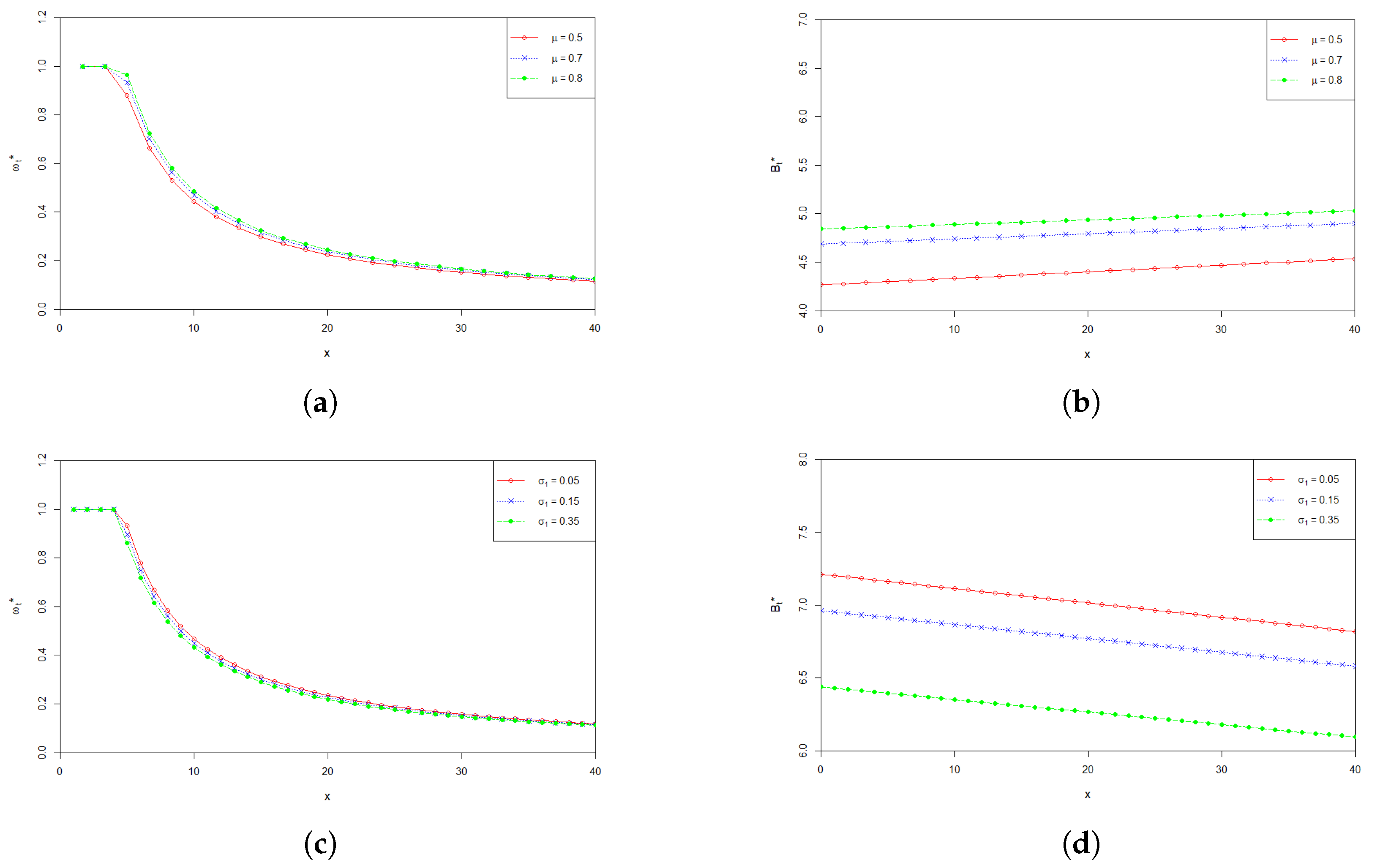
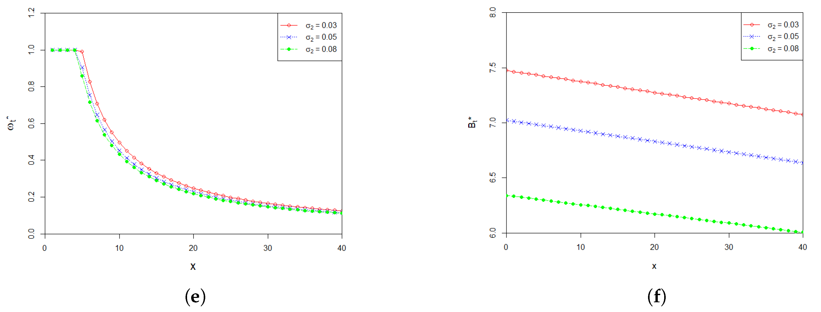
Effects of model main parameters , and on and are shown in Figure 2. The graphs in Figure 2a–f plot the values of the optimal investment proportion and the optimal payment rate with respect to the wealth x at time 0, when the parameters , and influencing the stock’s price change. From Figure 2a,b, we can find that the values of and increase as increases. This is consistent with the intuition that when the return rate of the stock becomes higher, the pension fund manager would naturally like to invest more in the stock to make more profit. At the same time, the pension fund manager is able to pay more to the retirees who participate in the plan. From Figure 2c–f, we can see that and decrease as and increases, respectively. The corresponding economic explanation is as follows. Higher values of and represent higher uncertainty of the fluctuation of the price of the stock. In other words, the higher the values of and are, the more risky the stock is. Therefore, a risk averse pension fund manager would most likely to reduce the amount invested in the stock, and has to lower the payment rate to the pension members because of the reduction of the profit from the stock market.
7. Conclusions
In this paper, we have proposed a new optimal control model for uncertain systems. Unlike the classic optimal control model for uncertain systems, the proposed new optimal control model takes into account environmental factors. Under the optimistic value criterion, we have established the principle and equation of optimality. As an example, an application to DC pension plans has been given to illustrate the proposed optimal control model for uncertain systems. Numerical studies are also given to show the sensitivity analysis of the optimal solution to the model parameters. For further topics, it would be interesting to consider the principle and equation of optimality under other optimality criteria such as the Hurwitz criterion.
Author Contributions
Conceptualization, W.L.; Supervision, Y.H.; Writing—original draft, W.W. and X.T. All authors have read and agreed to the published version of the manuscript.
Funding
This research was funded by National Natural Science Foundation of China grant number 11961064.
Conflicts of Interest
The authors declare no conflict of interest.
References
- Merton, R. Optimum consumption and portfolio rules in a continuous-time model. J. Econ. Theory 1971, 3, 373–413. [Google Scholar] [CrossRef] [Green Version]
- Fleming, W.; Rishel, R. Deterministic and Stochastic Optimal Control; Springer: New York, NY, USA, 1975. [Google Scholar]
- Whittle, P. Optimization over Time: Dynamic Programming and Stochastic Control; Wiley: New York, NY, USA, 1983. [Google Scholar]
- Boulier, J.; Trussant, E.; Florens, D. A dynamic model for pension funds management. In Proceedings of the Fifth AFIR International Colloquium, Brussels, Belgium, 7–8 September 1995; pp. 361–384. [Google Scholar]
- Yong, J.; Zhou, X. Stochastic Controls: Hamiltonian Systems and HJB Equations; Springer: New York, NY, USA, 1999. [Google Scholar]
- Taksar, M. Optimal risk and dividend distribution control models for an insurance company. Math. Methods Oper. Res. 2000, 51, 1–42. [Google Scholar] [CrossRef]
- Yang, H.; Zhang, L. Optimal investment for insurer with jump-diffusion risk process. Insur. Math. Econ. 2005, 37, 615–634. [Google Scholar] [CrossRef]
- Schmidli, H. Stochastic Control in Discrete Time. In Stochastic Control in Insurance; Springer: London, UK, 2008. [Google Scholar]
- Bjork, T.; Murgoci, A. A general theory of markovian time inconsistent stochastic control problems. SSRN Electron. J. 2010, 336, 1694759. [Google Scholar] [CrossRef] [Green Version]
- Fleming, W.H.; Soner, H.M. Controlled Markov Process and Viscosity Solutions; Springer: New York, NY, USA, 2010. [Google Scholar]
- Josa-Fombellida, R.; Rinco-Zapatero, J. Stochastic pension funding when the benefit and the risky asset follow jump diffusion processes. Eur. J. Oper. Res. 2012, 220, 404–413. [Google Scholar] [CrossRef]
- He, L.; Liang, Z. Optimal investment strategy for the DC plan with the return of premiums clauses in a mean variance framework. Insur. Math. Econ. 2013, 53, 643–649. [Google Scholar] [CrossRef]
- Guan, G.; Liang, Z. Optimal management of DC pension plan in a stochastic interest rate and stochastic volatility framework. Insur. Math. Econ. 2014, 57, 58–66. [Google Scholar] [CrossRef]
- Sun, J.; Li, Z.; Zeng, Y. Precommitment and equilibrium investment strategies for defined contribution pension plans under a jump-diffusion model. Insur. Math. Econ. 2016, 67, 158–172. [Google Scholar] [CrossRef]
- Nkeki, C.; Mcaleer, M. Optimal investment and optimal additional voluntary contribution rate of a DC pension fund in a jump diffusion environment. Ann. Financ. Econ. 2018, 12, 1750017. [Google Scholar] [CrossRef]
- Zhao, P.; Zhou, B.; Wang, J. Non–Gaussian Closed Form Solutions for Geometric Average Asian Options in the Framework of Non-Extensive Statistical Mechanics. Entropy 2018, 20, 71. [Google Scholar] [CrossRef] [Green Version]
- Mwanakatwe, P.; Song, L.; Hagenimana, E.; Wang, X. Management strategies for a defined contribution pension fund under the hybrid stochastic volatility model. Comput. Appl. Math. 2019, 38, 45. [Google Scholar] [CrossRef]
- Lima, L. Nonlinear Stochastic Equation within an It? Prescription for Modelling of Financial Market. Entropy 2019, 21, 530. [Google Scholar] [CrossRef] [PubMed] [Green Version]
- Lindgren, J. Efficient Markets and Contingent Claims Valuation: An Information Theoretic Approach. Entropy 2020, 22, 1283. [Google Scholar] [CrossRef] [PubMed]
- Zhang, X.; Guo, J. Optimal defined contribution pension management with salary and risky assets following jump diffusion processes. East Asian J. Appl. Math. 2020, 10, 22–39. [Google Scholar]
- Liu, B. Uncertainty Theory, 2nd ed.; Springer: Berlin, Germany, 2007. [Google Scholar]
- Liu, B. Fuzzy process, hybrid process and uncertain process. J. Uncertain Syst. 2008, 2, 3–16. [Google Scholar]
- Liu, B. Some research problems in uncertainty theory. J. Uncertain Syst. 2009, 3, 3–10. [Google Scholar]
- Liu, B. Uncertainty Theory: A Branch of Mathematics for Modeling Human Uncertainty; Springer: Berlin, Germany, 2010. [Google Scholar]
- Liu, B. Uncertainty Theory, 5th ed.; Springer: Berlin, Germany, 2020. [Google Scholar]
- Sheng, L.; Zhu, Y. Optimistic value model of uncertain optimal control. Int. J. Uncertain. Fuzziness Knowl.-Based Syst. 2013, 21 (Suppl. 01), 75–87. [Google Scholar] [CrossRef]
- Deng, L.; Chen, Y. Optimal control of uncertain systems with jump under optimistic value criterion. Eur. J. Control 2017, 38, 7–15. [Google Scholar] [CrossRef]
- Zhu, Y. Uncertain optimal control with application to a portfolio selection model. Cybern. Syst. Int. J. 2010, 41, 535–547. [Google Scholar] [CrossRef]
- Zhu, Y. Uncertain fractional differential equations and an interest rate model. Math. Methods Appl. Sci. 2015, 38, 3359–3368. [Google Scholar] [CrossRef]
- Zhu, Y. Uncertain Optimal Control; Springer Nature: Singapore, 2019. [Google Scholar]
- Deng, L.; Shen, J.; Chen, Y. Hurwicz model of uncertain optimal control with jump. Math. Methods Appl. Sci. 2020, 43, 10054–10069. [Google Scholar] [CrossRef]
- Huang, X.; Di, H. Uncertain portfolio selection with background risk. Appl. Math. Comput. 2016, 276, 284–296. [Google Scholar] [CrossRef]
- Li, B.; Zhu, Y.; Sun, Y.; Aw, G.; Teo, K. Multi-period portfolio selection problem under uncertain environment with bankruptcy constraint. Appl. Math. Model. 2018, 56, 539–550. [Google Scholar] [CrossRef] [Green Version]
- Lu, Z.; Yan, H.; Zhu, Y. European option pricing model based on uncertain fractional differential equation. Fuzzy Optim. Decis. Mak. 2019, 18, 199–217. [Google Scholar] [CrossRef]
- Jin, T.; Sun, Y.; Zhu, Y. Time integral about solution of an uncertain fractional order differential equation and application to zero-coupon bond model. Appl. Math. Comput. 2020, 372, 124991. [Google Scholar] [CrossRef]
- Liu, Y.; Yang, M.; Zhai, J.; Bai, M. Portfolio selection of the defined contribution pension fund with uncertain return and salary: A multi-period mean-variance model. J. Intell. Fuzzy Syst. 2018, 34, 2363–2371. [Google Scholar] [CrossRef]
- Deng, L.; You, Z.; Chen, Y. Optimistic value model of multidimensional uncertain optimal control with jump. Eur. J. Control 2018, 39, 1–7. [Google Scholar] [CrossRef]
- Deng, L.; Zhu, Y. Uncertain optimal control with jump. ICIC Express Lett. Part B Appl. 2012, 3, 419–424. [Google Scholar]
Figure 1.
(a) Effect of on the optimal investment proportion ; (b) Effect of on the optimal payment rate .
Figure 1.
(a) Effect of on the optimal investment proportion ; (b) Effect of on the optimal payment rate .

Figure 2.
(a) Effect of on the optimal investment proportion ; (b) Effect of on the optimal payment rate ; (c) Effect of on the optimal investment proportion ; (d) Effect of on the optimal payment rate ; (e) Effect of on the optimal investment proportion ; (f) Effect of on the optimal payment rate .


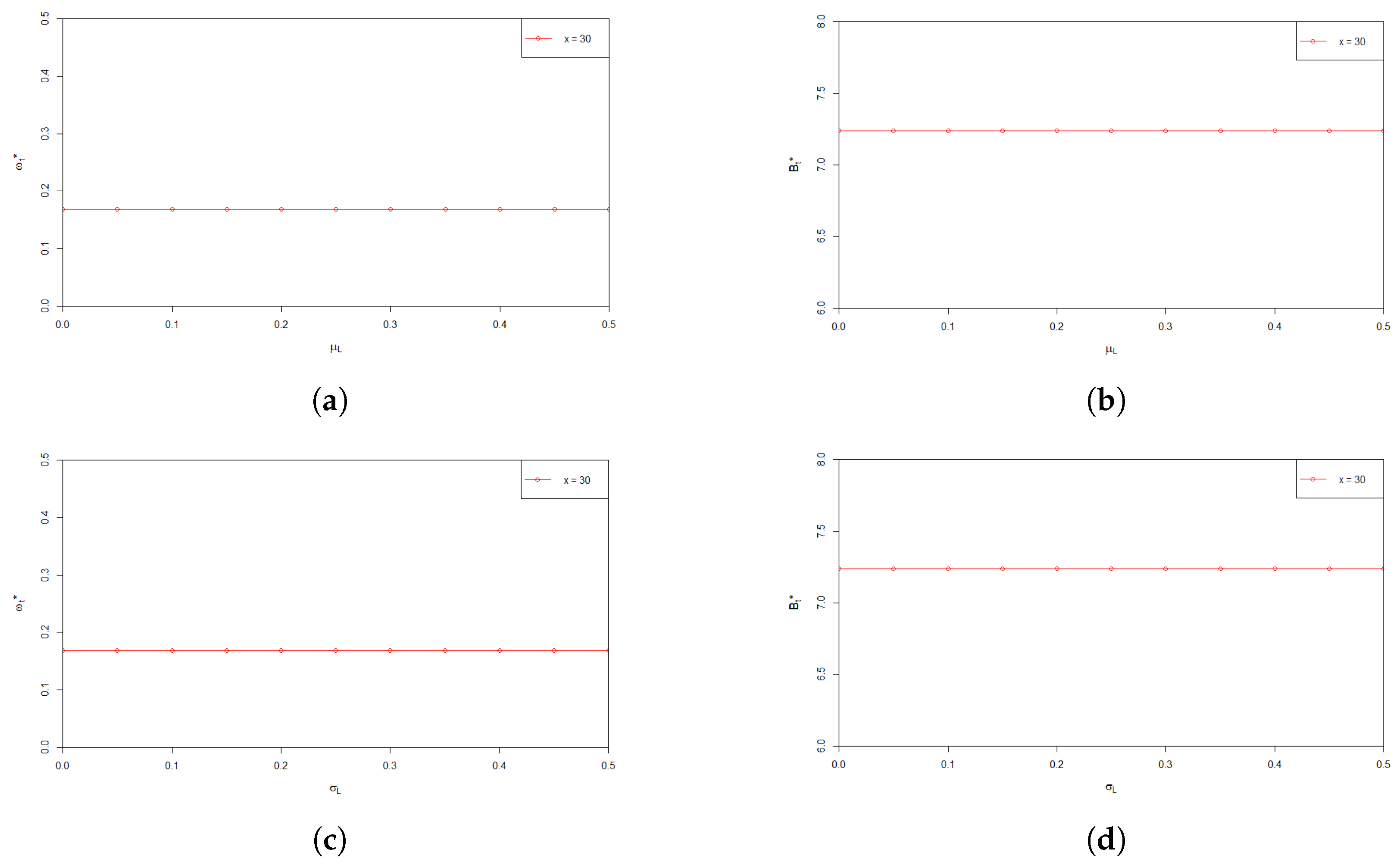
Figure 3.
(a) Effect of on the optimal investment proportion ; (b) Effect of the optimal payment rate ; (c) Effect of on the optimal investment proportion ; (d) Effect of the optimal payment rate .
Figure 3.
(a) Effect of on the optimal investment proportion ; (b) Effect of the optimal payment rate ; (c) Effect of on the optimal investment proportion ; (d) Effect of the optimal payment rate .

Publisher’s Note: MDPI stays neutral with regard to jurisdictional claims in published maps and institutional affiliations. |
© 2022 by the authors. Licensee MDPI, Basel, Switzerland. This article is an open access article distributed under the terms and conditions of the Creative Commons Attribution (CC BY) license (https://creativecommons.org/licenses/by/4.0/).
Share and Cite
MDPI and ACS Style
Liu, W.; Wu, W.; Tang, X.; Hu, Y. Optimal Control of Background-Based Uncertain Systems with Applications in DC Pension Plan. Entropy 2022, 24, 734. https://0-doi-org.brum.beds.ac.uk/10.3390/e24050734
AMA Style
Liu W, Wu W, Tang X, Hu Y. Optimal Control of Background-Based Uncertain Systems with Applications in DC Pension Plan. Entropy. 2022; 24(5):734. https://0-doi-org.brum.beds.ac.uk/10.3390/e24050734
Chicago/Turabian StyleLiu, Wei, Wanying Wu, Xiaoyi Tang, and Yijun Hu. 2022. "Optimal Control of Background-Based Uncertain Systems with Applications in DC Pension Plan" Entropy 24, no. 5: 734. https://0-doi-org.brum.beds.ac.uk/10.3390/e24050734
Note that from the first issue of 2016, this journal uses article numbers instead of page numbers. See further details here.