The Stochastic Stationary Root Model


Department of Economics, University of Copenhagen, 1353 Copenhagen K, Denmark
Econometrics 2018, 6(3), 39; https://0-doi-org.brum.beds.ac.uk/10.3390/econometrics6030039
Submission received: 31 March 2018
/
Revised: 27 July 2018
/
Accepted: 13 August 2018
/
Published: 21 August 2018
(This article belongs to the Special Issue Celebrated Econometricians: Katarina Juselius and Søren Johansen)
Abstract
:We propose and study the stochastic stationary root model. The model resembles the cointegrated VAR model but is novel in that: (i) the stationary relations follow a random coefficient autoregressive process, i.e., exhibhits heavy-tailed dynamics, and (ii) the system is observed with measurement error. Unlike the cointegrated VAR model, estimation and inference for the SSR model is complicated by a lack of closed-form expressions for the likelihood function and its derivatives. To overcome this, we introduce particle filter-based approximations of the log-likelihood function, sample score, and observed Information matrix. These enable us to approximate the ML estimator via stochastic approximation and to conduct inference via the approximated observed Information matrix. We conjecture the asymptotic properties of the ML estimator and conduct a simulation study to investigate the validity of the conjecture. Model diagnostics to assess model fit are considered. Finally, we present an empirical application to the 10-year government bond rates in Germany and Greece during the period from January 1999 to February 2018.
Keywords:
cointegration; particle filtering; random coefficient autoregressive model; state space model; stochastic approximationJEL Classification:
C15; C32; C51; C581. Introduction
In this paper, we introduce the multivariate stochastic stationary root (SSR) model. The SSR model is a nonlinear state space model, which resembles the Granger-Johansen representation of the cointegrated vector autoregressive (CVAR) model, see inter alia Johansen (1996) and Juselius (2007). The SSR model decomposes a p–dimensional observation vector into r stationary components and nonstationary components, which is similar to the CVAR model. However, the roots of the stationary components are allowed to be stochastic; hence the name ‘stochastic stationary root’. The stationary and nonstationary dynamics of the model are observed with measurement error, which in this model prohibits close-form expressions for e.g., the log-likelihood, sample score and observed Information matrix. Likelihood-based estimation and inference therefore calls for non-standard methods.
Although the SSR model resembles the CVAR model, it is differentiated by its ability to characterize heavy-tailed dynamics in the stationary component. Heavy-tailed dynamics, and other types of nonlinear dependencies, are not amenable to analysis with the CVAR model, which has prompted work into nonlinear alternatives, see inter alia Bohn Nielsen and Rahbek (2014), Kristensen and Rahbek (2013), Kristensen and Rahbek (2010), and Bec et al. (2008). Similarly, cointegration in the state space setting has been considered in term of the common stochastic trend (CST) model by Chang et al. (2009) as well as the CVAR model with measurement errors by Bohn Nielsen (2016). Additionally, the SSR model is also related to the stochastic unit root literature, see inter alia Granger and Swanson (1997), Leybourne and McCabe (1996), Lieberman and Phillips (2014), Lieberman and Phillips (2017), McCabe and Tremayne (1995), and McCabe and Smith (1998). Relevant empirical applications where the SSR model could potentially provide a better fit than the CVAR model include, but are not limited to, (i) log-prices of assets that exhibit random walk behavior in the levels and heavy-tailed error-correcting dynamics in the no-arbitrage relations, and (ii) interest rates for which the riskless rate exhibits random walk-type dynamics and the risk premia undergo periods of high levels and high volatility.
The stationary and nonstationary components of the SSR model are treated as unobserved processes, and consequently need to be integrated out in order to compute the log-likelihood function and its derivatives. Due to the nonlinearity of the model, this cannot be accomplished analytically. We appeal to the incomplete data framework and the simulation-based approach known as particle filtering to approximate the log-likelihood function, sample score and observed Information matrix. See inter alia Gordon et al. (1993), Doucet et al. (2001), Cappé et al. (2005), and Creal (2012) for an overview of the particle filtering literature. Moreover, we rely on stochastic approximation methods to obtain the maximum likelihood (ML) estimator, see Poyiadjis et al. (2011). Summarizing, the main contributions of this paper are to
- i
- introduce and study the SSR model, and
- ii
- propose a method for approximate frequentist estimation and inference.
It is beyond the scope of this paper to provide a complete proof of the asymptotic properties of the ML estimator. The study of the asymptotic properties of the ML estimator in general state space models, such as the SSR model, is an emerging area of research. Most existing results rely on compactness of the state space, which excludes the SSR model and is generally restrictive. For results in this direction, see e.g., Olsson and Rydén (2008) who derive consistency and asymptotic normality for the ML estimator by discretizing the parameter space. Douc et al. (2011) have shown consistency of the ML estimator without assuming compactness, but the regularity conditions are nonetheless too restrictive to encompass the SSR model. Instead of providing a complete proof of the asymptotic properties of the ML estimator, we conjecture the asymptotic properties of the derivatives of the log-likelihood function. We base the conjecture on known properties of models that are closely related to the SSR model, and corroborate it by a simulation study. Given the conjecture holds, it allows us to establish the asymptotic properties of the ML estimator. We leave proving the conjecture for future work, and focus in this paper on developing methods for approximate frequentist estimation and inference.
The rest of the paper is organized as follows. We introduce the SSR model in Section 2, and study some properties of the process in Section 3. In Section 4 we introduce likelihood-based estimation and inference for the unknown model parameter. In Section 5 we introduce the incomplete data framework. In Section 6 we introduce the particle filter-based approximations to the log-likelihood function, sample score and Information matrix. In Section 7 we propose how to approximate the ML estimator and classic standard errors. In Section 8 we consider model diagnostics. In Section 9 we conduct a simulation study of the asymptotic distribution of the ML estimator. In Section 10 we apply the SSR model to monthly observations of 10-year government bond rates in Germany and Greece from January 1999 to February 2018. We conclude in Section 11. All proofs have been relegated to Appendix B, while Appendix A contains various auxiliary results.
Notation-wise, we adopt the convention that the ‘blackboard bold’ typeface, e.g., , denotes operators, and the ‘calligraphy’ typeface, e.g., , denotes sets. We thus let and denote the real and natural numbers, respectively. For any matrix A, we denote by the determinant, by the Euclidean norm, and by the spectral radius. For some positive definite matrix A, we let denote the lower triangular Cholesky decomposition. For some function , let denote the derivative of with respect to z. For some stochastic variable with Gaussian distribution with mean and covariance , let denote the Gaussian probability density function evaluated at z. We let denote the probability density of stochastic variable with respect to the –dimensional Lebesgue measure m, while denotes the corresponding probability measure. Additionally, the letter ‘p’ is generic notation for probability density functions and measures induced by the model defined in (1)–(3) below. The ‘bold’ typeface, e.g., , is generic notation for analytically intractable quantities, in the sense of having no closed-form expression. Finally, we denote a sequence of real –dimensional vectors by .
2. The Model
The structure of the SSR model is similar to the Granger-Johansen representation of the CVAR model, cf. Johansen (1996, chp. 4), but departs from it in two respects. First, the stationary component is a random coefficient autoregressive process, cf. e.g., Feigin and Tweedie (1985), rather than an autoregressive process. Second, the stationary and nonstationary components are observed with measurement error. This makes the SSR model is a state space model, whereas the CVAR model is observation-driven. In addition to resembling the CVAR model, the SSR model constitutes an extension of the CST model, cf. Chang et al. (2009). However, while the CST model is a linear Gaussian state space model, the SSR model is a nonlinear Gaussian state space model as it allows the stationary component to be a random coefficient autoregressive process.
Formally, we consider the observable p-dimensional discrete time vector process , for given by,
for fixed initial values and , and with , and mutually independent. We define with . The sequences and are unobserved and take values and for . Additionally, the matrices are of dimensions and , with and invertible. Let the random coefficient, , be i.i.d. Gaussian,
with a positive definite covariance matrix. Let the observation error be i.i.d. Gaussian, such that with a positive definite matrix, and let the innovations and be jointly Gaussian such that and with cross-covariance , such that the joint covariance matrix,
is positive definite. Let all the introduced matrices be of appropriate dimensions and full rank. Furthermore, we introduce the orthogonal complements to A and B, which we denote and , such that and with b and a of full column rank. Finally, we let .
Define the parameter vectors,
which contain the parameters governing the observations , and unobserved components and , respectively. The parameter vectors take values in and , respectively. Additionally, we define the full parameter vector as
which indexes the model, and we refer to as the parameter space. Note that and in are variation free in the sense of Engle et al. (1983). The parameter space is a subset of the -dimensional Euclidean space , where denotes the number of elements in . In the case where no restrictions are imposed on , the dimension increases rapidly in r due to the parameters in . We suggest restricting the off-diagonal elements of to zero to avoid over-parameterization. The number of parameters is then when the model is otherwise unrestricted.
The log-likelihood function for any parameter vector , fixed initial values , and , and observation sequence is given by,
3. Properties of the Process
In this section we consider some properties of the process defined by Equations (1)–(3) for a given parameter value . Specifically, we study the nonstationary and stationary components, including conditions on the parameter that ensure strict stationarity of the stationary component. Additionally, we decompose the observation into nonstationary and stationary directions.
3.1. The Unobserved Components
The first component of the model, , is a random walk (RW) in dimensions, equivalently expressed as an autoregressive process with a unit root. That is, for ,
with . The process (11) admits the transition density with respect to the –dimensional Lebesgue measure; however, it does not have a stationary distribution. This type of process has been studied extensively, see e.g., Dickey and Fuller (1979). In summary, the RW process is linear and Gaussian, but nonstationary.
The second unobserved component of the model, , is a random coefficient autoregressive (RCAR) process of lag order one in r dimensions. The RCAR process (2)–(3) is observationally equivalent to a double autoregressive (DAR) process with one lag, cf. Ling (2007), which we formalize in Lemma 1.
Lemma 1.
The DAR representation in Lemma 1 of the RCAR process in (2)–(3) characterizes the process dynamics in terms of the conditional mean and variance. The conditional mean is autoregressive. However, the conditional variance depends positively on the lagged level ‘squared’. The conditional variance is heteroskedastic, but not in the well-known ARCH sense of e.g., Engle (1982); rather, the lagged level of the process enters the variance, not the lagged innovation . To illustrate the point, we consider for a moment the conditional variance in the univariate case , which is given by . Here we see that a relatively large (in absolute terms) lagged level will result in a relatively large volatility in the present period, and vice versa.
We make the following assumption on the random coefficients (3) in order to ensure strict stationarity of the RCAR process (2)–(3).
Assumption 1.
Assume that the top Lyapunov exponent is strictly negative,
Remark 1.
The top Lyapunov exponent (14) is intractable but can be approximated to arbitrary precision via simulation, cf. inter alia Ling (2007) and Francq and Zakoian (2010). The following approximation converges almost surely
as . In turn, can be computed efficiently via the QR-decomposition, cf. Dieci and Van Vleck (1995).
Assumption 1 ensures that the RCAR process can be characterized as a geometrically ergodic Markov chain, cf. Meyn and Tweedie (2005). This is formalized in the following theorem.
Theorem 1
(Feigin and Tweedie (1985), Theorem 3). Under Assumption 1, the process is geometrically ergodic. In particular, the initial value can be given an initial distribution such that is stationary and geometrically ergodic with some fractional moment.
Remark 2.
The stationary component, , exhibits heavy-tailed behavior since it satisfies a stochastic recurrence equation. Pedersen and Wintenberger (2018) have recently considered the tail properties of processes of the form (2) for a more general specification of the random coefficient, , that includes BEKK-ARCH and DAR-type processes as special cases. It should be possible to show that the stationary distribution of as defined in (2)–(3) also has power-law tails under suitable conditions.
3.2. The Observed Process
The observations are conditionally independent given the sequence of unobserved components . Thus, the dynamics of the observed process are determined by the dynamics of the unobserved components.
We use the orthogonal complements and of the loading matrices B and A, respectively, and the skew-projection identity of Johansen (1996) to decompose the observation vector as follows,
where we define and . Here and are invertible thanks to our assumption that is square and invertible. By premultiplying by we eliminate the stationary directions, while leaving the nonstationary directions,
What is left after the linear transformation (17) is a random walk with Gaussian measurement error. Similarly, premultiplying by eliminates the nonstationary directions while the stationary directions remain,
The process given by (18) is a stationary random coefficient autoregressive process with Gaussian measurement error.
The decomposition of the observation process (16) allows for a cointegration interpretation of the SSR model. The p observed variables in share common stochastic trends (17) with loading matrix , while the r linear combinations (18) are stationary and load into the levels with the matrix . The observed process admits the conditional density with respect to the p–dimensional Lebesgue measure; however, this density does not have a closed-form expression. Moreover, the observed process does not have a stationary distribution.
4. Likelihood-Based Estimation and Inference
In this section, we introduce the ML estimator and consider its asymptotic properties. We wish to conduct estimation and inference based on the true, but intractable, model likelihood. Due to the intractability of the likelihood, we can neither compute the ML estimator via numerical optimization of (8), nor compute classic standard errors via the observed Information matrix (10). We refer to the ML estimator as being ‘doubly intractable’, with reference to the concept from the literature in Bayesian statistics on models with intractable likelihoods, see e.g., Murray et al. (2006). It is beyond the scope of this paper to derive a full asymptotic theory for the SSR model. Instead, we conjecture the limiting properties of the likelihood function (8) and its derivatives (9)–(10). We obtain the asymptotic properties for the ML estimator based on the conjecture.
We recall preliminarily that the ML estimator is defined as the parameter vector that maximizes the log-likelihood function (8),
noting that the ML estimator (19) is a function of the observation sequence . We denote by the true parameter value for the data generating process (1)–(3). In the following, we make the below conjecture on the asymptotic properties of (8)–(10). Note that, having assumed that is known, the score, information, and likelihood in the conjecture refer to the unknown parameters only; that is, all elements in excluding .
Conjecture 1.
If Assumption 1 holds, is known, and , then the log-likelihood function is three times continuously differentiable in θ, and
- 1.
- as , with ,
- 2.
- as , with , and
- 3.
- ,
where is a neighborhood of and , , as .
Remark 3.
Theorem 3 in Bohn Nielsen and Rahbek (2014) shows that Conjecture 1 holds in the case of the strictly stationary bivariate double autoregressive model with BEKK-type time-varying covariance. With known, the SSR model corresponds closely to this model plus Gaussian measurement errors.
It should be noted that we propose Conjecture 1 despite lack of finite moments of the RCAR process, cf. Theorem 1. This is in line with the results of inter alia Bohn Nielsen and Rahbek (2014) for the bivariate DAR model, and Ling (2004, 2007) for the univariate DAR model.
The result in Theorem 2 below states that if Conjecture 1 holds true, then the ML estimator (19) is unique, –consistent and asymptotically Gaussian. The result follows from applying Lemma 1 in Jensen and Rahbek (2004), the conditions of which correspond to (1.)–(3.) of Conjecture 1.
Theorem 2
(Jensen and Rahbek (2004), Lemma 1). If Conjecture 1 holds, then there exists a fixed open neighborhood of the true parameter , which is an interior point of Θ, such that with probability tending to one as , there exists a minimum point in and is convex in . In particular, is unique and satisfies the score equation
Additionally, the ML estimator is consistent , and asymptotically Gaussian,
Proof.
Conjecture 1 satisfies the Cramer-type conditions of Lemma 1 in Jensen and Rahbek (2004), which provides the result. ☐
We assume that the true value of B is known, because Chang et al. (2009) showed that the ML estimator of the loading matrix B exhibits T-convergence and is asymptotically mixed Gaussian in the CST model. The CST model corresponds to the SSR model with , but without the stationary components, i.e., for any p. We find it reasonable to believe that this result carries over to the SSR model. Moreover, fixing B is conceptually similar to classic cointegration analysis with known cointegrating vectors, which is an accepted starting point for new methodological developments, see e.g., Bec and Rahbek (2004). In applications we often have a predefined set of cointegrating vectors that we are interested in. In the context of the SSR model, the cointegrating vectors correspond to the rows of the orthogonal complement . As an example, for the empirical illustration in Section 10 we consider an interest rate spread in a bivariate system with one common stochastic trend, i.e., and . The spread implies , which in turn corresponds to the loading matrix when normalizing on the first element.
The Fisher Information matrix, , is consistently estimated by the (scaled) observed Information matrix evaluated at , cf. Conjecture 1.(3.). Moreover, the asymptotic variance of the score, , is equal to the Fisher Information matrix when the model is well-specified; the information matrix equality holds, cf. e.g., Hamilton (1994, sct. 14.4). In this case, the asymptotic variance of the ML estimator (19) is simply the inverse Fisher Information matrix. Thus, we can use classic standard errors, that are based on the observed Information matrix (10), to conduct inference on the ML estimates.
5. The Incomplete Data Framework
In this section, we appeal to the incomplete data framework of Dempster et al. (1977) to deal with the unobserved components of the SSR model. We first formulate the state space representation of the model in (1)–(3) and its associated optimal filtering problem. Secondly, we formulate the intractable sample score (9) and observed information matrix (10) in terms of the optimal filtering problem. In Section 6 we introduce a particle filter algorithm with which we can approximate the optimal filtering problem. This enables approximation of the intractable sample score and observed information matrix via the particle filter algorithm.
5.1. The State Space Form and the Optimal Filtering Problem
Preliminarily, we collect the unobserved components in the vector , which we refer to as the state vector. The unobserved components are Markov, see (11)–(13), and the observation depends only on the contemporary values of the unobserved components. Thus, the SSR model in (1)–(3) has the dependency structure of a state space model. Formally, for , the SSR model in (1)–(3) has the following state space representation,
with and fixed, and , and and mutually independent. We define accordingly,
and recall that is defined in Lemma (1). We refer to (22) as the observation equation, and to (23) as the transition equation. It is easy to verify that the state space representation in (22) and (23) is observationally equivalent to the SSR model as presented in (1)–(3). The observation and transition equations admit the densities with respect to the p-dimensional Lebesgue measure,
respectively. We refer to (25) as the observation density and to (26) as the transition density. As mentioned previously, we suppress the dependence on the initial observation .
One approach to conducting inference on the unobserved components, i.e., the state vector , is the optimal filtering problem, cf. Anderson and Moore (1979). The optimal filtering problem refers to the general problem of computing the conditional expectation of some sequence of unobserved states given some sequence of observations. In the following, we consider the specific instance of the optimal filtering problem known as the smoothing problem. Formally, the smoothing problem is a conditional expectation of the form,
for any function and point in time . We refer to the function as the test function and to the density as the smoothing density. The test function may be time-varying, but of known form for a fixed observation sequence . The smoothing density in (27) can be expressed as the recursion of the lagged smoothing density,
initialized with . The normalizing constant in (28) is the likelihood contribution, which is given by the integral,
5.2. The Sample Score and Observed Information as Smoothing Problems
The incomplete data framework is closely associated with the classic expectation maximization (EM) algorithm, introduced in Dempster et al. (1977). The EM algorithm is a common approach to maximizing the log-likelihood function (8) to obtain the ML estimator (19) for models with unobserved variables. When the EM algorithm is applicable, it is also possible to evaluate the sample score (9) and observed Information matrix (10). For the SSR model, however, the EM algorithm does not apply directly, yet we may use the incomplete data framework to reformulate the sample score and observed Information in terms of intractable smoothing problems of the form (27).
A central concept of the EM algorithm is the auxiliary function called the intermediate quantity, which is defined as,
where
for any parameter values . We refer to as the complete data log-likelihood. By the state space model structure (22)–(23) and variation freeness of defined in (7), we have that the complete data log-likelihood is given by,
The intermediate quantity (30) is sometimes also called the expected log-likelihood, since it is interpretable as the conditional expectation of the complete data log-likelihood (32) given the observations . We note the term separating the log-likelihood (8) and the intermediate quantity (30) is the entropy of the smoothing density (28) with parameters and , defined in (31).
We are interested in the intermediate quantity (30) because it provides a convenient way to derive the sample score and observed Information matrix in terms of the derivatives of the complete data log-likelihood (32). The first and second derivatives of the complete data log-likelihood function in (32) are the sum of the first and second order derivatives of the observation and transition log-densities with respect to and , respectively. These can be computed by either analytical or numerical differentiation of (32). For , we define the derivatives of (32) in terms of the functions,
where, taking advantage of the variation freeness of the model parameter, , we define the summands of (33) and (34), respectively, as
and
We note that the functions (35) and (36) should not be confused with the measurement error in (22) and innovations in (23), respectively.
If the first and second order derivatives of the complete data log-likelihood in (33) and (34), respectively, are integrable with respect to the smoothing density (28), then we may appeal to Fisher’s and Louis’ identities (defined below) to express the sample score (9) and observed Information matrix (10) in terms of smoothing problems of the form (27).
Conjecture 2.
For any and observation sequence , it holds that and .
For the same reasons we conjectured the asymptotic properties of the true log-likelihood function, sample score, observed information matrix, we conjecture integrability of the derivatives of the complete data log-likelihood (33) and (34).
Fisher’s identity, cf. Dempster et al. (1977), states the first derivative of the intermediate quantity (30) is equivalent to the sample score (9). Similarly, Louis’ identity of Louis (1982) establishes a relation between the first and second derivatives of the intermediate quantity (30) and the observed Information matrix (10).
Lemma 2
Although Lemma 2 shows the sample score (9) and observed Information (10) can be restated as smoothing problems of the form (27), we still cannot obtain closed-form expressions due to the intractability of the optimal filtering problem, cf. Section 5.1. In the next section, we introduce a particle filter algorithm that can approximate smoothing problems for appropriately chosen test functions, such as the functions and under Conjecture 2.
6. Particle Filter-Based Approximations
In this section, we introduce a particle filter algorithm that produces pointwise approximations to the true but intractable log-likelihood function (8), sample score (9), and observed Information matrix (10) for any parameter and fixed observation sequence . In Section 7, we show how to apply the particle filter-based approximations introduced in this section to approximate the true, intractable ML estimator and classic standard errors, which we introduced in Section 4.
6.1. Particle Filtering
A particle filter is a simulation-based algorithm that produces approximations to smoothing problems of the form (27) for state space models. We introduce here a standard particle filter, which produces empirical measures that recursively approximate the smoothing density (28) for each time point in the observed sample . The empirical measures consist of point masses, which we refer to as particles, and we use these for Monte Carlo integration in order to approximate the smoothing problem (27). Additionally, the particle filter produces a point-wise approximation of the log-likelihood function as a by-product. For an introduction to particle filtering in the context of economics and finance see Creal (2012).
The particle filter algorithm relies on an importance density, denoted , that has the same support and recursive structure as the smoothing density (28). Formally, for , we define the importance density as,
initialized by . We note the importance density (41) is defined recursively by , which we refer to as the importance transition density.
Assuming the smoothing density (28) is absolutely continuous with respect to the importance density (41), we can write the former as a the product of the importance density and a weight function,
We refer to the weight function as the normalized importance weight. We note that (42) constitutes a change of measure from the smoothing density to the importance density, and the normalized importance weight is a Radon-Nikodym derivative between the two densities.
Substituting the recursive expressions for the smoothing density (28) and importance density (41) into the expression for the normalized importance weight in (42), we obtain a recursive expression for the normalized importance weight,
where we define
We refer to (44) as the incremental importance weights. The recursion for the normalized importance weight (43) is normalized by the likelihood contribution (29) and is therefore also intractable.
For particle filtering in general, the importance transition density is subject to choice under mild regularity conditions, cf. e.g., Assumption 9.4.1 in Cappé et al. (2005). We let the importance transition density be the corresponding model density; formally,
We refer to (45) as the locally optimal transition density. This choice of importance transition density is optimal in the sense that it is conditional on the the contemporary observation , cf. Doucet et al. (2000). This is sometimes also referred to as ‘fully adapted’, cf. e.g., Pitt and Shephard (1999b). If we instead let the importance transition density be the model transition density (26), we omit the information about that is contained in . The locally optimal transition density is not necessarily available in closed-form for nonlinear state space models. It is, however, available for the SSR model and we present it in Lemma 3.
Lemma 3.
For , the locally optimal transition density has the closed-form expression
where the conditional mean and variance are given by,
with
and the state space form definitions given in (24).
Remark 4.
The locally optimal transition density (46) is related to the Kalman (1960) filter, which solves the optimal filtering problem analytically for linear and Gausian models. Equations (49)–(52) correspond the Kalman filter for a known value of . Related methods for efficient particle filtering include the mixture Kalman filter and Rao-Blackwellisation, cf. Chen and Liu (2000) and Andrieu and Doucet (2002).
It is straightforward to use the general expression for the incremental importance weight in (44) to show that letting the importance transition density be the locally optimal transition density, i.e., (45), results in the following specific expression for incremental importance weights,
We refer to the density in (53) as the predictive observation density. It has a closed-form expression that follows from the closed-form expression of the locally optimal transition density in Lemma 3.
Corollary 1.
Proof.
Contained in the proof of Lemma 3. ☐
Remark 5.
The choice of importance transition density (45) is locally optimal in the sense that the conditional variance of the incremental importance weights (53) given is zero, cf. Doucet et al. (2000).
The particle filter, presented in Algorithm 1 below, produces weighted particle samples approximately distributed as the smoothing density (28) at each point in time . The algorithm consists of iterating over three steps. At point t in time, the first step is to sample N particles, denoted , from the importance density (41) given the particle sample from . This is called the propagation step. Step two consists of computing self-normalized importance weights, denoted , that approximate the normalized importance weights (43). This is the weighting step. The third step is to sample N particle indices, denoted , with replacement. We sample index j with probability for . We retain the number of particles indicated by the resulting sample of particle indices, denoted , and let the importance weights be uniform. This is the resampling step. After resampling, we store the particle samples and proceed to .
For a fixed parameter value and observation sequence , we run the locally optimal particle filter for the SSR model as specified in Algorithm 1 below.
| Algorithm 1: Locally Optimal Particle Filter. |
Given a parameter , initialize by setting and for . For :
|
Remark 6.
The resampling method applied in step (3.) of Algorithm 1 is known as multinomial resampling. Alternative methods that are guaranteed to produce lower Monte Carlo variance exists, cf. Douc et al. (2005). We consider multinomial resampling for its analytical tractability, and recommend applying one of the more efficient alternatives in practice.
Remark 7.
The notation is ambiguous due to the resampling step of Algorithm 1, since the elements of the ith particle path at time , denoted , are not necessarily the same as the first elements of the ith particle path at time t, denoted . By convention, always refers to the particle chain after resampling at time t (similarly refers to the chain before resampling). We refer to elements k to l of the ith particle chain after resampling at time t as .
The particle filter in Algorithm 1 produces two particle samples at each point in time, t. The first set, , is produced at the propagation step (1.) and is associated with importance weights in the weighting step (2.), . The second set, , is produced at the resampling step (3.). Both sets are approximately drawn from the smoothing density (28). We note the resampling step introduces additional sampling error, cf. Chopin (2004), so we calculate approximations using the weighted sample unless otherwise specified.
The particle filter iterates over over the propagation, weighting and resampling steps throughout the sequence, , after which the algorithm terminates. We note the two sets of particles produced during each iteration are themselves random variables measurable with respect to the sub--algebras and , defined next.
Definition 1.
Define the sub-σ-algebras , for , initialized by .
At each point in time, we associate an empirical measure with the weighted particle sample generated by the propagation (1.) and reweighting (2.) steps in Algorithm 1. Formally, for , we define the empirical measure,
where denotes the point measure at with respect to . The weighted particles that constitute the empirical measure (59) are approximately distributed according to the smoothing density (28). We emphasize the weighted particles are not independent draws from (28), because the resampling step introduces dependence between the particles at each iteration of the algorithm. We use the empirical measure (59) to define a particle filter-based approximation of the intractable smoothing problem in (27),
for any point in time . Due to dependence between the weighted particles, we cannot establish the asymptotic properties of the approximation (60) based on the law of large numbers and central limit theorem for independent random variables. For appropriately chosen test functions , the approximation (60) is both consistent and asymptotically Gaussian as the number of particles tends to infinity, , cf. Theorem 9.4.5 in Cappé et al. (2005).
The particle filter in Algorithm 1 also produces an approximation of the log-likelihood function (8) evaluated at the parameter value and the observation sequence ,
We note that the approximate log-likelihood function (61) consists of the logarithm of the product of normalizing constants produced by Algorithm 1. The approximate log-likelihood (61) is consistent in the sense that it converges in probability to the true log-likelihood function, as the number of particles tends to infinity, see Lemma 4.
Lemma 4.
6.2. The Approximate Sample Score and Observed Information Matrix
We showed in Section 5 that the sample score and observed Information matrix can be expressed in terms of smoothing problems of the form (27). Appealing to Fisher’s identity (37) in Lemma 2, and to the approximation of the smoothing problem (60), we define the particle filter-based approximate sample score as,
for any parameter , with the function as defined in (33). If Conjecture 2 holds, then the approximate sample score in (63) is both consistent and asymptotically normal.
Lemma 5.
If Conjecture 2 holds and , then the approximate sample score (63) is asymptotically normal,
as . An intractable expression for the asymptotic covariance matrix is given in Lemma A.5 by setting and .
Similarly, by appealing to Louis’ identity (38) in Lemma 2, and to the approximation of the smoothing problem (60), we define the particle filter-based approximate observed Information matrix as,
for any parameter , where we define the approximations to (39) and (40) as
and the functions and are defined in (33) and (34), respectively. If Conjecture 2 holds, then the approximate observed Information in (65) is consistent, stated in the following lemma.
Lemma 6.
If Conjecture 2 holds and , then the approximate observed Information matrix (65) is consistent,
as .
Both the approximate sample score (63) and observed Information matrix (65) are biased for finite N. This is a general issue related to the particle filter-based approximation of the smoothing problem (60). At each iteration, the particle filter in Algorithm 1 relies on an approximation of the normalized constant, i.e., likelihood contribution. This induces a finite-sample bias in (60) that gradually disappears as the number of particles N tends to infinity and is negligible for large enough N, cf. e.g., Robert and Casella (2010, sct. 3.3.2).
The particle filter-based approximation of the sample score (63) and observed Information matrix (65) correspond to a batch version of Algorithm A in Poyiadjis et al. (2011), which is of computational cost , but exhibits quadratically increasing variance of the approximate sample score as a function of the sample size T. We note that Poyiadjis et al. (2011) also suggest an alternative algorithm, that exhibits linearly increasing variance as a function of T, but at the computational cost . For smaller sample sizes, such as monthly observations as usually encountered in economics, we have found that the algorithm is adequate.
7. Particle Filter-Based Estimation and Inference
In this section, we show how the approximate sample score (63) and observed Information matrix (65) can be used to perform parameter estimation and inference. We apply a stochastic approximation method based on the approximate sample score to approximate the ML estimator (19). This has recently been suggested in Poyiadjis et al. (2011). We then use the approximate observed Information matrix to obtain approximate standard errors for the approximate ML estimates. Although these quantities are ‘approximate’, we note that they can be made arbitrarily precise by increasing the number of particles, N, at the expense of increased computational effort.
Recall from Section 4 that the ML estimator (19) is doubly intractable. Consequently, we cannot apply gradient-based optimization algorithms to maximize the log-likelihood function (8). Originally proposed in Robbins and Monro (1951), stochastic approximation methods are conceptually similar to gradient-based optimization methods, but rely on noisy rather than exact evaluations of the sample score to optimize the objective function. The basic idea is that appropriately decreasing the step sizes provides an averaging of the random errors induced by the noisy evaluations of the sample score. For a book-length treatment of stochastic approximation, we refer to Kushner and Yin (2003).
The stochastic approximation algorithm proposed in Poyiadjis et al. (2011, sct. 3.1) consists of a recursion that is conceptually similar to the steepest descent method, cf. e.g., Nocedal and Wright (2006, chp. 3). Prior to executing the algorithm, we choose a fixed initial parameter value , a sequence of particle counts , a sequence of step sizes , and a sequence of weight matrices . The particle counts must be monotonically increasing positive integers, the step sizes must be strictly positive, non-summable but square summable,
and the weight matrices must be positive definite. Having chosen the initial parameter, particle counts, step sizes, and weight matrices, we run the recursion,
for . Here K has to be sufficiently large in the sense that the sequence of parameter values generated by the recursion (70) has stabilized in a neighborhood of the true ML estimate. Additionally, if the particle count is large enough, the approximation error affecting the stochastic approximation recursion (70) will be approximately normal, cf. Lemma 5. In this case large disturbances will be rare, such that the parameter sequence is likely to stabilize without exhibiting large jumps.
We denote by the particle paths produced by the particle filter in Algorithm 1 at iteration j of the stochastic approximation recursion (70). The iteration index j is notationally identical to time index of the particle path, cf. Remark 7. Although this is abuse of notation, it is clear from the context whether we refer to the parameter iteration or particle path time index. The parameter produced by iteration j of (70) is a random variable that is measurable with respect to the sub--algebra , defined next.
Definition 2.
Let denote the sub-σ-algebra in Definition 1 generated with the parameter value , and define the sub-σ-algebras for , initialized by .
One of the main benefits of the stochastic approximation method is that the method is known to stabilize for a wide variety of initial values, sample counts, step sizes, and weight matrices. In practice, all of these choices affect the number of iterations needed to bring the parameter sequence into the neighborhood of the true ML estimator. The choice of step sizes is particularly important, since large step sizes generally speed up the convergence, but fail to dampen the approximation-induced noise. Small step sizes reduce the noise, but cause slow convergence. The particle count has a similar effect, since a low number of particles will result in a computationally cheap but noisy approximation of the sample score, while a large number of particles reduces the noise but increases the computational cost. Heuristically, it is appropriate to use a combination of large step sizes and small particle counts until the parameter sequence has reached a neighborhood of the ML estimator, and then switch to a combination of smaller step sizes and larger particle counts to reduce the noise. The intuition is that, while far away from the ML estimator, a relatively noisy approximation of the sample score will still on average lead the algorithm in the right direction.
The presence of noise in the sample score is not an impediment when applying stochastic approximation, since the use of decreasing step sizes provides an averaging of the errors. However, the finite sample bias of the particle filter-based approximate sample score, cf. Section 6.2, poses a problem since its effect is not mitigated by decreasing the step sizes. Bias reduction is possible by increasing the particle count together with the iteration number j.
The stochastic approximation method is presented in Algorithm 2 below.1
| Algorithm 2: Stochastic Approximation. |
Choose the initial parameter , the particle counts , the step sizes and weighting matrices . For :
|
Polyak (1990) and Polyak and Juditsky (1992) showed that if the step sizes satisfy the summability conditions (69) and tend to zero slower than , then the average of the last iterations converges at an optimal rate. Here denotes the iteration number at which the averaging begins; implicitly, we discard the initial iterations. We define the approximate ML estimator as,
suppressing the dependence on the particle count. Establishing convergence of the approximate ML estimator (73) to the true ML estimator (19) is outside the scope of this paper. However, if (73) converges in probability to (19) for any fixed T, then (73) inherits the consistency property, cf. Theorem 2, of the true ML estimator.
Convergence of the particle filter-based stochastic approximation method proposed in Poyiadjis et al. (2011) has, to the author’s knowledge, not been studied yet. The finite-sample bias of the approximate sample score (63) presents the primary obstacle to establishing convergence results. Intuition suggests that increasing the number of particles with the iteration number j solves the problem. However, convergence of such schemes has not been carefully established, cf. Douc et al. (2014, sct. 12.1.2). Poyiadjis et al. (2011) report stabilization of the particle filter-based stochastic approximation method with constant particle count. In Section 10, we report similar stabilization with increasing particle counts.
If the model is correctly specified, we would conduct inference on the ML estimator via the observed Information matrix, cf. Section 4. Analogously, since the approximate observed Information matrix (65) converges in probability to the true observed Information matrix (10), we can conduct inference for the approximate ML estimator (73) via the approximate observed Information matrix (65), the same way we would conduct inference given the true observed Information matrix (10).
8. Model Diagnostics
In this section, we introduce a method to conduct model diagnostics, such that we may assess whether the SSR model is well-specified for a given parameter and observation sequence . Recall that the disturbances , and are normally distributed and serially independent with mean zero and unit variances. Because the components and are hidden to us, we cannot directly compute the residuals corresponding to the disturbances. Instead, we introduce the normalized one-step prediction errors, cf. Durbin and Koopman (2012, sct. 2.12), that can be approximated via particle filtering. This approach to model diagnostics for state space models has also previously been considered in Pitt and Shephard (1999a).
We define the normalized one-step prediction errors as,
for . For a well-specified model, the sequence of normalized one-step prediction errors should be serially independent with mean zero with unit variance. Any deviation from these characteristics are indicative of model misspecification.
The conditional mean and variance in (74) can be stated in terms of smoothing problems, where the test functions are the conditional mean and variance of the predictive observation density,
We note that the conditional mean and variance of the predictive observation density are given in Lemma 3. Using the locally optimal particle filter in Algorithm 1, we define approximations to (75) and (76) as
respectively, where we have defined the conditional moments given each individual particle as,
for . Finally, we use the approximations (77) and (78) to define the approximate normalized likelihood contributions as follows,
for . Thus, by applying the particle filter in Algorithm 1, we obtain the sequence of approximate normalized one-step prediction errors via (77)–(81). For N sufficiently large, we can use the sequence to test whether the true sequence of normalized one-step prediction errors is serially independent with mean zero and unit variance. For common tests for serial dependence and ARCH effects see e.g., Doornik and Hendry (2013, sct. 11.9.2–3).
9. Simulation Study
In this section, we conduct a simulation study of the asymptotic properties of the ML estimator, stated in Theorem 2. We limit our treatment to B, A, and , leaving aside the remaining parameters , , , and . Recall, the loading matrix for the stationary components A is conjectured to be asymptotically normal, while the loading matrix of the nonstationary components B is kept fixed. Due to the results of Chang et al. (2009), we expect the asymptotic distribution of B to be mixed normal, and we tentatively investigate this. Moreover, we consider the case where is a stochastic unit root. A deterministic unit root is associated with the Dickey-Fuller distribution, cf. Dickey and Fuller (1979), while a stochastic unit root has been shown to be asymptotically normal, see e.g., Ling (2007) and Bohn Nielsen and Rahbek (2014).
Recall, Theorem 2 is based on the conjectured properties of the true, intractable log-likelihood function and its derivatives, cf. Conjecture 1. The aim is to substantiate this conjecture by obtaining the distribution of the approximate ML estimator based on simulated data sets. Usually, the number of realizations in a simulation study of this type is in excess of 1000 and the sample length in excess of 2500 observations. Due to the computational intensity of the particle filter-based stochastic approximation method in Algorithm 2, we limit ourselves to 250 realizations and 500 observations.
We let each of the simulated data sets be a bivariate series of length observations with stationary component and nonstationary component. We use the parameter
to generate the simulated data sets. We note the parameter values (83) result in a top Lyapunov coefficient of , computed via (15) with , such that the RCAR process is strictly stationary.
Having simulated 250 series with the data generating process given by (1)–(3) and (83), we apply Algorithm 2 with iterations to obtain the approximate ML estimate for the parameter in question, e.g., , keeping all other parameters fixed at the true values in (83). We initialize the algorithm at the true parameter value, and initiate Polyak averaging at iteration .2 Moreover, we let the particle count increase as
where denotes the largest integer that is smaller than the argument. We let the step size sequence to decrease as
and set the weight matrix to
for . Note the particle count (84) tends to infinity as , eliminating the finite-sample bias of (63)–(65), the step sizes satisfy (69), and the weight matrix is constant.3
The results from the simulation experiment are presented in Figure 1. Despite the relatively low number of realizations and observations, Figure 1 is instructive of the asymptotic distributions of , and , cf. Panels (a), (c) and (d). These all appear to be normal. Recall, Theorem 2 does not state the asymptotic distribution of the ML estimator for , and from Panel (b) it does not appear to be normal. Rather, the realizations in Panel (b) are consistent with mixed normality, as we would expect from the closely-related CST model, cf. Chang et al. (2009). To investigate further, one could to simulate the t-ratios of , which should be standard normal. This involves the approximation of the observed Information matrix for each realization, which further increases the computational cost. For this reason, and because we consider B fixed, we do not pursue this further here.
In summary, the findings of the simulation study tentatively support the conjecture made in Section 4. Namely, the ML estimator for A, and is asymptotically normal. The ML estimator for appears to be consistent with mixed normality. We have not investigated the remaining parameters.
10. An Illustration
In this section, we illustrate the use of the SSR model by applying it to the monthly 10-year government bond rates for Germany and Greece from January 1999 to February 2018.4 We denote the German and Greek bond rates and , respectively, and measure these in basis points per year. The sample begins at the introduction of the euro area and ends at present day. During this period, the rates initially exhibit convergence towards a common ‘euro area rate’, until interrupted by the euro area crisis beginning in 2009 and culminating in 2011. The rates, the spread and the changes in the spread are illustrated in Figure 2 below. Because the spread is up to 75 times larger during the second half of the sample than during the first half, we split the display of the sample into the first and second half, respectively.
Panels (a) and (b) in Figure 2 show the bond rates, Panels (c) and (d) show the spread, and Panels (e) and (f) show the changes in the spread in the two periods. We note two features of the observations. First, Panel (a) suggests the rates can be characterized by a shared common stochastic trend, since these tend to move in tandem. Second, Panels (d) and (f) suggest the spread can be characterized by a RCAR process, since the changes in the spread, cf. Panel (f), are clearly positively associated with the level of the spread itself, cf. Panel (d).
We define the observation vector as . We condition on the observation for January 1999, which we denote , such that the effective sample spans . From visual inspection of Figure 2, our working assumption is that the spread is strictly stationary, while the rates share a common stochastic trend. With a dimensional system, we thus have stationary component and nonstationary component. Moreover, we fix , such that the orthogonal complement produces the spread. To ensure the model is just-identified, we normalize on the second element of A, such that .
We apply the particle filter-based stochastic approximation method in Algorithm 2 to obtain the approximate ML estimate of the model parameter . For this illustration, we run the algorithm for iterations. We let the particle count increase as (84), the step size sequence decrease as (85), and the weighting matrix as (86). We initiate Polyak averaging at iteration .
Figure 3 shows the results of running the particle filter-based stochastic approximation method. Panel (a) displays the iterations for the parameters in the observation Equation (22), Panel (b) displays the iterations for the parameters in the transition Equation (23), and Panel (c) displays the sequence of realized approximate log-likelihoods together with a moving average of lag order 500. The algorithm has been implemented in the Ox 7 programming language, cf. Doornik (2012), using analytical derivatives of the complete data log-likelihood (32) for the evaluation of the function (33). The elements of the parameter sequence shown in Panels (a) and (b) have stabilized after the initial 7500 iterations. At the th iteration, the particle count has increased to 550, the step size decreased to , and the sequences have stabilized. By inspection of the sequence of the approximate log-likelihood in Panel (c), we see that the value has also stabilized after approximately 7500 iterations.
The estimation results are presented in Table 1, together with approximate classic standard errors.5 Before considering inference, we assess the model fit. We compute the normalized one-step prediction errors via (81) using particles. Table 2 presents univariate tests for autocorrelation (AR) of order one and two, autoregressive conditional heteroskedasticity (ARCH) of order one, and a multivariate test for AR of order one and two, cf. Doornik and Hendry (2013, sct. 11.9.2–3). We cannot reject the null hypothesis of no-AR of order one and two in the univariate as well as multivariate tests at a critical level. Nor can we reject the null hypothesis of no-ARCH for the residuals at a critical level. However, we note the test for the German rate is close to, but below, our chosen critical level. This could suggest unmodeled heteroskedasticity in the German bond rate. In conclusion, the overall specification of the model is acceptable. Moreover, computing the top Lyapunov coefficient via (15) with produces a coefficient of , which indicates the stationary direction is strictly stationary for .
The model is reasonably well-specified, and we therefore proceed to use the approximate classic standard errors to conduct inference on the approximate ML estimates. First, we note the standard error of the estimate of is extremely small. Since the test for no-ARCH for the residuals associated with the German rate is rejected at the critical level, this could affect the approximate classic standard errors.6 Nevertheless, it is economically plausible that the stationary component also loads into the German rate, given that a large increase in the Greek rate would in this case coincide with a small drop in the German rate, which is consistent with risk-averse investors seeking safer assets in times of uncertainty, such as the euro area crisis. Second, we cannot reject the null hypothesis that at a critical level with . Third, the estimate of is significantly different from zero at any commonly used critical level. However, the constant term is not significantly different from zero with . Fourth, the measurement errors are highly positively correlated with coefficient , and the innovations of the unobserved components are highly negatively correlated with coefficient . The results in Table 1 suggest the level of the stationary direction is a stochastic unit root process without a constant term. An approximate likelihood ratio test for the joint null hypothesis fails to reject the null at a critical level with .
Based on the estimates in Table 1, we use the orthogonal complements b and a to compute the changes of the nonstationary and stationary components, given by and , respectively. These are illustrated in Figure 4. First, we note the magnitude of the changes in Panels (a) and (b) of Figure 4 are slightly larger during the second half of the sample than during the first (standard deviations and , respectively). Otherwise, the series in Panels (a) and (b) in Figure 4 are consistent with a homoskedastic random walk plus measurement error, cf. (17). The magnitude of the changes in Panels (c) and (d) of Figure 4 is positively associated with the level, just as observed in Figure 2. This is consistent with a random coefficient autoregressive process plus measurement error, cf. (18).
Summarizing, the empirical illustration suggests that the SSR model successfully characterizes the 10-year government bond rates for Germany and Greece during the period from January 1999 to February 2018. During this sample, the spread exhibits bubble-like behavior, which is captured by the random coefficient autoregressive dynamics of the stationary component. Additionally, the levels exhibit a shared common stochastic trend, which is captured by the random walk dynamics of the nonstationary component.
11. Conclusions
In this paper, we have proposed and studied the stochastic stationary root model, which is a multivariate nonlinear state space model. We introduced particle filter-based approximations of the intractable log-likelihood function, sample score and observed Information matrix. In turn, we used these to approximate the ML estimator via stochastic approximation, and showed how to perform inference via the approximate observed Information matrix. We considered model diagnostics to assess the model fit. Additionally, we conducted a simulation study to investigate the asymptotic properties of the ML estimator. Finally, we presented an empirical application to the 10-year government bond rates in Germany and Greece in the period from January 1999 to February 2018 to illustrate the usefulness of the SSR model.
Acknowledgments
The author gratefully acknowledges comments by two anonymous referees that have led to substantial improvements of the paper. The author also thanks the editors, Rocco Mosconi and Paolo Paruolo, for constructive feedback, and the assistant editor, Lu Liao, for assisting in the publication process. Finally, the author would like to thank Anders Rahbek, Michael Pitt, Siem Jan Koopman, Heino Bohn Nielsen, Katarina Juselius, Søren Johansen, Simon Hetland, Gareth Roberts, Adam Johansen, Axel Finke, and Anthony Lee for helpful comments and dicsussions. Part of the work was undertaken while the author was a PhD student at the Department of Economics at the University of Copenhagen and part of the work was undertaken while the author was a CRiSM Research Fellow at the Department of Statistics at the University of Warwick. While at the University of Warwick, funding from the 36 Engineering and Physical Sciences Research Council (EPSRC) is gratefully acknowledged (Grant EP /D002060/1). All errors and omissions are the sole responsibility of the author.
Conflicts of Interest
The author declares no conflict of interest.
Appendix A. Auxiliary Results
Proof of Lemma A.1.
By Corollary 1 we have that is Gaussian, and therefore strictly positive for all and , which yields part (i). Moreover, because the observation density (25) is Gaussian with constant and non-singular covariance matrix, we obtain part (ii). ☐
Proof of Lemma A.2.
Preliminarily, we observe the likelihood in (A1) can equivalently be written in terms of the complete data likelihood ,
which, by the state space structure of the model, cf. (25)–(26), is equivalently
By Lemma A.1.(i) and (A3), we have that the likelihood in (A1) is strictly positive, since
Moreover, by Lemma A.1.(ii), the likelihood in (A1) is also finite, since
which completes the proof of Lemma A.2. ☐
Proof of Lemma A.3.
We preliminarily note that the locally optimal transition density (46) can be written as
where the predictive observation density is given by the integral,
By (A6) and the definition of absolute continuity, part (i) states that for every Borel-measurable set , it holds that
By (A7) and Lemma A.1.(i), we know the predictive observation density is strictly positive for all and . Therefore (A8) is true for all and , and part (i) holds.
To show part (ii), we first use (A6) to write
where, by Corollary 1, we have that is Gaussian and therefore strictly positive for all and , and part (ii) holds.
Part (iii) follows from being Gaussian, cf. Lemma 3, and therefore strictly positive for all . Thus, part (iii) holds. ☐
Lemma A.4.
Proof of Lemma A.4.
We apply Theorem 9.4.5.(i) in Cappé et al. (2005) by verifying its conditions, i.e., Assumptions 9.4.1–3. We note the theorem is stated for scalar test functions, but generalizes to higher-dimensional test functions. Assumptions 9.4.1–2 is hold by Lemma A.1, while Assumption 9.4.3 holds by Lemma A.3. Thus, the conditions for Theorem 9.4.5.(i) in Cappé et al. (2005) are satisfied, which completes the proof of Lemma A.4. ☐
Lemma A.5.
If and , then it holds that the approximation (60) is consistent and asymptotically normal,
for any , as . Initialized by , the asymptotic covariance matrix is given by
where, for any appropriately integrable function , we define the operators
omitting dependence on θ.
Proof of Lemma A.5.
We apply Theorem 9.4.5.(ii) in Cappé et al. (2005) by verifying its conditions, i.e., Assumptions 9.4.1–3. Similar to the proof of Lemma A.4, we note the theorem is stated for scalar test functions, but generalizes to higher-dimensional test functions. Assumptions 9.4.1–2 is hold by Lemma A.1, while Assumption 9.4.3 holds by Lemma A.3. Thus, the conditions for Theorem 9.4.5.(ii) in Cappé et al. (2005) are satisfied, which completes the proof of Lemma A.5. ☐
Appendix B. Main Results
Proof of Lemma 1.
We compute conditional mean and variance of in Equation (2). First the mean
and then the variance
Since the conditional distribution of given is Gaussian, it is completely characterized by its first and second conditional moments. Thus, we obtain equations (12)–(13), which completes the proof of Lemma 1. ☐
Proof of Lemma 2.
The result is an application of the Fisher’s and Louis’ identities to the SSR model. We use Proposition 10.1.6 in Cappé et al. (2005), by verifying the conditions.
First, we verify that Assumption 10.1.3 in Cappé et al. (2005) holds. We have that is an open subset of , which satisfies Assumption 10.1.3.(i). Assumption 10.1.3.(ii) is satisfied via Lemma A.2. Assumption 10.1.3.(iii) is encompassed by condition (b) of Proposition 10.1.6 in Cappé et al. (2005), shown below. Thus, Assumption 10.1.3 in Cappé et al. (2005) holds.
Second, we verify conditions (a) and (b) of Proposition 10.1.6 in Cappé et al. (2005). Condition (a) holds by Conjecture 1. For condition (b), we begin with the third and last part, which states that
For , the complete data log-likelihood (32) is log-Gaussian and therefore continuous with respect to , and (A17) holds.
The second part of condition (b) states that for ,
which is holds by Conjecture 2.
The first part of condition (b) states that for , the entropy function in (31) is twice-differentiable with respect to for fixed and . Using (A17) and that the complete data log-likelihood (32) is twice-differentiable with respect to , we have that (31) is also twice-differentiable with respect to . Thus, Proposition 10.1.6 in Cappé et al. (2005) applies for the SSR model, which completes the proof of Lemma 2. ☐
Proof of Lemma 3.
Define the conditional moments of the locally optimal transition density (46),
Applying the Gaussian projection, we can write these as
where we have used that,
We define the conditional moments of the predictive observation density,
where we have used (22). Similarly, we define the conditional moments of the transition density,
where we have used (23), which concludes the proof of Lemma 3. ☐
Proof of Lemma 4.
Lemma A.4 establishes that Theorem 9.4.5 in Cappé et al. (2005) holds. It is a corollary to Theorem 9.4.5 in Cappé et al. (2005) that
as . By continuity of the logarithm, the continuous mapping theorem and the definitions (8) and (61), we therefore have that,
as , which completes the proof of Lemma A.4. ☐
Proof of Lemma 5.
We apply Lemma A.5 for setting the test function to , cf. (33). By Conjecture 2 we have that , which satisfies the condition, and Lemma A.5 applies. ☐
Proof of Lemma 6.
We apply Lemma A.4 to the functions , and the outer product for . First, Conjecture 2 implies that , such that by setting the test function to , Lemma A.4 gives us that,
as . Second, Conjecture 2 states , such that by setting the test function to , Lemma A.4 gives us that,
as . Third, we note that by the Cauchy-Schwarz inequality it holds that,
such that, by Conjecture 2, we have that
Thus, by setting the test function to , Lemma A.4 gives us that,
as . Now, by (37), (39), (40), (63), (66), and (67), we have that (A30)–(A34) correspond to,
as , respectively, such that we get by the continuous mapping theorem that,
as , which completes the proof of Lemma 6. ☐
References
- Anderson, Brian D. O., and John B. Moore. 1979. Optimal Filtering. Upper Saddle River: Prentice-Hall, pp. 1–367. [Google Scholar]
- Andrieu, Christophe, and Arnaud Doucet. 2002. Particle filtering for partially observed Gaussian state space models. Journal of the Royal Statistical Society B 64: 827–36. [Google Scholar] [CrossRef]
- Bec, Frederique, and Anders Rahbek. 2004. Vector Equilibrium Correction Models with Non-Linear Discontinuous Adjustments. Econometrics Journal 7: 628–51. [Google Scholar] [CrossRef]
- Bec, Frédérique, Anders Rahbek, and Neil Shephard. 2008. The ACR Model: A Multivariate Dynamic Mixture Autoregression. Oxford Bulletin of Economics and Statistics 70: 583–618. [Google Scholar] [CrossRef]
- Cappé, Olivier, Eric Moulines, and Tobias Rydén. 2005. Inference in Hidden Markov Models. New York: Springer. [Google Scholar]
- Chang, Yoosoon, J. Isaac Miller, and Joon Y. Park. 2009. Extracting a Common Stochastic Trend: Theory with Some Applications. Journal of Econometrics 150: 231–47. [Google Scholar] [CrossRef]
- Chen, Rong, and Jun S. Liu. 2000. Mixture Kalman Filters. Journal of the Royal Statistical Society: Series B (Statistical Methodology) 62: 493–508. [Google Scholar] [CrossRef]
- Chopin, Nicolas. 2004. Central Limit Theorem for Sequential Monte Carlo Methods and its Application to Bayesian Inference. The Annals of Statistics 32: 2385–411. [Google Scholar] [CrossRef]
- Creal, Drew. 2012. A Survey of Sequential Monte Carlo Methods for Economics and Finance. Econometric Reviews 31: 245–96. [Google Scholar] [CrossRef]
- Dempster, Arthur P., Nan M. Laird, and Donald B. Rubin. 1977. Maximum Likelihood from Incomplete Data via the EM Algorithm. Journal of the Royal Statistical Society: Series B (Statistical Methodology) 37: 1–38. [Google Scholar]
- Dickey, David A., and Wayne A. Fuller. 1979. Distribution of the Estimators for Autoregressive Time Series with a Unit Root. Journal of the American Statistical Association 74: 427–31. [Google Scholar]
- Dieci, Luca, and Erik S. Van Vleck. 1995. Computation of a Few Lyapunov Exponents for Continuous and Discrete Dynamical Systems. Applied Numerical Mathematics 17: 275–91. [Google Scholar] [CrossRef]
- Doornik, Jurgen A., and David F. Hendry. 2013. Modelling Dyamic Systems—PcGive 14: Volume II. London: Timberlake Consultants Ltd., pp. 1–284. [Google Scholar]
- Doornik, Jurgen A. 2012. Developer’s Manual for Ox 7. London: Timberlake Consultants Ltd., pp. 1–182. [Google Scholar]
- Douc, Randal, Olivier Cappé, and Eric Moulines. 2005. Comparison of Resampling Schemes for Particle Filtering. Paper presented at the 4th International Symposium on Image and Signal Processing and Analysis, Zagreb, Croatia, September 15–17; pp. 64–69. [Google Scholar]
- Douc, Randal, Eric Moulines, Jimmy Olsson, and Ramon Van Handel. 2011. Consistency of the Maximum Likelihood Estimator for General Hidden Markov Models. The Annals of Statistics 39: 474–513. [Google Scholar] [CrossRef]
- Douc, Randal, Eric Moulines, and David Stoffer. 2014. Nonlinear Time-Series: Theory, Methods, and Applications with R Examples. Boca Raton: CRC Press. [Google Scholar]
- Doucet, Arnaud, and Neil Shephard. 2012. Robust Inference on Parameters via Particle Filters and Sandwich Covariance Matrices. Economics Series Working Papers 606. Oxford, UK: University of Oxford. [Google Scholar]
- Doucet, Arnaud, Nando De Freitas, Kevin Murphy, and Stuart Russell. 2000. Rao-Blackwellised Particle Filtering for Dynamic Bayesian Networks. In Proceedings of the 16th Conference on Uncertainty in Artificial Intelligence. San Francisco: Morgan Kaufmann Publishers Inc. [Google Scholar]
- Doucet, Arnaud, Nando de Freitas, and Neil Gordon. 2001. Sequential Monte Carlo Methods in Practice. New York: Springer. [Google Scholar]
- Durbin, James, and Siem Jan Koopman. 2012. Time Series Analysis by State Space Methods, 2nd ed. Oxford: Oxford University Press. [Google Scholar]
- Engle, Robert F., David F. Hendry, and Jean-Francois Richard. 1983. Exogeneity. Econometrica 51: 277–304. [Google Scholar] [CrossRef]
- Engle, Robert F. 1982. Autoregressive Conditional Heteroscedasticity with Estimates of the Variance of United Kingdom Inflation. Econometrica 50: 987–1007. [Google Scholar] [CrossRef]
- Feigin, Paul D., and Richard L. Tweedie. 1985. Random Coefficient Autoregressive Processes: A Markov Chain Analysis of Stationarity and Finiteness of Moments. Journal of Time Series Analysis 6: 1–14. [Google Scholar] [CrossRef]
- Francq, Christian, and Jean-Michel Zakoian. 2010. GARCH Models: Structure, Statistical Inference and Financial Applications. Hoboken: Wiley, p. 489. [Google Scholar]
- Gordon, Neil J., David J. Salmond, and Adrian F. M. Smith. 1993. Novel Approach to Nonlinear/Non-Gaussian Bayesian State Estimation. IEE Proceedings F, Radar and Signal Processing 140: 107–13. [Google Scholar] [CrossRef]
- Granger, Clive W. J., and Norman R. Swanson. 1997. An Introduction to Stochastic Unit-Root Processes. Journal of Econometrics 80: 35–62. [Google Scholar] [CrossRef]
- Hamilton, James Douglas. 1994. Time Series Analysis. Princeton: Princeton University Press. [Google Scholar]
- Jensen, Søren Tolver, and Anders Rahbek. 2004. Asymptotic Inference for Nonstationary GARCH. Econometric Theory 20: 1203–26. [Google Scholar] [CrossRef]
- Johansen, Søren. 1996. Likelihood-Based Inference in Cointegrated Vector Autoregressive Models (Advanced Texts in Econometrics). Oxford: Oxford University Press. [Google Scholar]
- Juselius, Katarina. 2007. The Cointegrated VAR Model: Methodology and Applications (Advanced Texts in Econometrics). Oxford: Oxford University Press. [Google Scholar]
- Kalman, Rudolph Emil. 1960. A New Approach to Linear Filtering and Prediction Problems. Transactions of the ASME–Journal of Basic Engineering 82: 35–45. [Google Scholar] [CrossRef] [Green Version]
- Kristensen, Dennis, and Anders Rahbek. 2010. Likelihood-based Inference for Cointegration with Nonlinear Error-Correction. Journal of Econometrics 158: 78–94. [Google Scholar] [CrossRef]
- Kristensen, Dennis, and Anders Rahbek. 2013. Testing and Inference in Nonlinear Cointegrating Vector Error Correction Models. Econometric Theory 29: 1238–88. [Google Scholar] [CrossRef]
- Kushner, Harold, and G. George Yin. 2003. Stochastic Approximation and Recursive Algorithms and Applications, 2nd ed. New York: Springer. [Google Scholar]
- Leybourne, Stephen J., Brendan P. M. McCabe, and Andrew R. Tremayne. 1996. Can Economic Time Series Be Differenced To Stationarity? Journal of Business & Economic Statistics 14: 435–46. [Google Scholar]
- Lieberman, Offer, and Peter C. B. Phillips. 2014. Norming rates and limit theory for some time-varying coefficient autoregressions. Journal of Time Series Analysis 35: 592–623. [Google Scholar] [CrossRef]
- Lieberman, Offer, and Peter C. B. Phillips. 2017. A multivariate stochastic unit root model with an application to derivative pricing. Journal of Econometrics 196: 99–110. [Google Scholar] [CrossRef]
- Ling, Shiqing. 2004. Estimation and Testing Stationarity for Double-Autoregressive Models. Journal of the Royal Statistical Society: Series B (Statistical Methodology) 66: 63–78. [Google Scholar] [CrossRef]
- Ling, Shiqing. 2007. A Double AR(p) Model: Structure and Estimation. Statistica Sinica 17: 161–75. [Google Scholar]
- Louis, Thomas A. 1982. Finding the Observed Information Matrix when Using the EM Algorithm. Journal of the Royal Statistical Society: Series B (Statistical Methodology) 44: 226–33. [Google Scholar]
- McCabe, Brendan P. M., and Richard J. Smith. 1998. The power of some tests for difference stationarity under local heteroscedastic integration. Journal of the American Statistical Association 93: 751–61. [Google Scholar] [CrossRef]
- McCabe, Brendan P. M., and Andrew R. Tremayne. 1995. Testing a time series for difference stationarity. Annals of Statistics 23: 1015–28. [Google Scholar] [CrossRef]
- Meyn, Sean P., and Richard L. Tweedie. 2005. Markov Chains and Stochastic Stability. Cambridge: Cambridge University Press. [Google Scholar]
- Murray, Iain, Zoubin Ghahramani, and David MacKay. 2006. MCMC for Doubly-Intractable Distributions. Paper presented at the Twenty-Second Conference on Uncertainty in Artificial Intelligence (UAI2006), Cambridge, MA, USA, July 13–16. [Google Scholar]
- Nocedal, Jorge, and Stephen Wright. 2006. Numerical Optimization, 2nd ed. New York: Springer. [Google Scholar]
- Olsson, Jimmy, and Tobias Rydén. 2008. Asymptotic Properties of Particle Filter-Based Maximum Likelihood Estimators for State Space Models. Stochastic Processes and Their Applications 118: 649–80. [Google Scholar] [CrossRef]
- Pedersen, Rasmus Søndergaard, and Olivier Wintenberger. 2018. On the tail behavior of a class of multivariate conditionally heteroskedastic processes. Extremes 21: 261–84. [Google Scholar] [CrossRef]
- Pitt, Mark, and Neil Shephard. 1999a. Time Varying Covariances: A Factor Stochastic Volatility Approach. In Bayesian Statistics. Edited by José M. Bernardo, James O. Berger, A. P. Dawid and Adrian F. M. Smith. Oxford: Oxford University Press, vol. 6, pp. 547–70. [Google Scholar]
- Pitt, Michael K., and Neil Shephard. 1999b. Filtering via Simulation: Auxiliary Particle Filters. Journal of the American Statistical Association 94: 590–99. [Google Scholar] [CrossRef]
- Polyak, Boris T., and Anatoli B. Juditsky. 1992. Acceleration of Stochastic Approximation by Averaging. SIAM Journal on Control and Optimization 30: 838–55. [Google Scholar] [CrossRef]
- Polyak, Boris Teodorovich. 1990. A New Method of Stochastic Approximation Type. Automation and Remote Control 51: 98–107. [Google Scholar]
- Poyiadjis, George, Arnaud Doucet, and Sumeetpal S. Singh. 2011. Particle Approximations of the Score and Observed Information Matrix in State Space Models with Application to Parameter Estimation. Biometrika 98: 65–80. [Google Scholar] [CrossRef]
- Robbins, Herbert, and Sutton Monro. 1951. A Stochastic Approximation Method. The Annals of Mathematical Statistics 22: 400–7. [Google Scholar] [CrossRef]
- Robert, Christian P., and George Casella. 2010. Introducing Monte Carlo Methods with R, 1st ed. New York: Springer, p. 296. [Google Scholar]
- Nielsen, Heino Bohn, and Anders Rahbek. 2014. Unit Root Vector Autoregression with Volatility Induced Stationarity. Journal of Empirical Finance 29: 144–67. [Google Scholar] [CrossRef]
- Nielsen, Heino Bohn. 2016. The Co-integrated Vector Autoregression with Errors-in-Variables. Econometric Reviews 35: 169–200. [Google Scholar] [CrossRef]
| 1. | We use the Choleski factorization to ensure positive definiteness of the covariance matrices , and . Thus, we estimate the parameters B, A, , , , and using Algorithm 2 and transform the covariances to the original parametrization. We obtain standard errors via the -method. |
| 2. | Because we initialize at the true parameter value, the parameter sequences stabilize within the first 100 realizations. Using iterations is sufficient to reduce the impact of the approximation error. |
| 3. | The choice of weight matrix is based on hand-tuning the convergence speed of Algorithm 2 by running a small number of trial-and-error runs with particles and constant step size . |
| 4. | Obtained via a Bloomberg LP Terminal using the ticker codes ‘GDBR10 Index’ and ‘GGGB10YR Index’. |
| 5. | The difference between computing the classic standard errors with and particles is negligible. |
| 6. | Particle filter-based approximate robust standard errors have been suggested in Doucet and Shephard (2012), but we do not pursue this idea further in the present context. |
Figure 1.
Simulation study with 250 realizations of the approximate MLE for , , , and .

Figure 2.
German and Greek 10-year government bond rates, spread and changes in the spread. Monthly observations in basis points from January 1999 to February 2018.
Figure 2.
German and Greek 10-year government bond rates, spread and changes in the spread. Monthly observations in basis points from January 1999 to February 2018.

Figure 3.
Parameter and log-likelihood sequences from stochastic approximation with iterations. We also show a moving average of lag order 500 for the log-likelihood sequence. To avoid large differences in the scales of the displayed sequences, we have scaled the sequences for , , , , and by 100, , , , and 2 respectively.

Figure 4.
Changes in the nonstationary and stationary components.


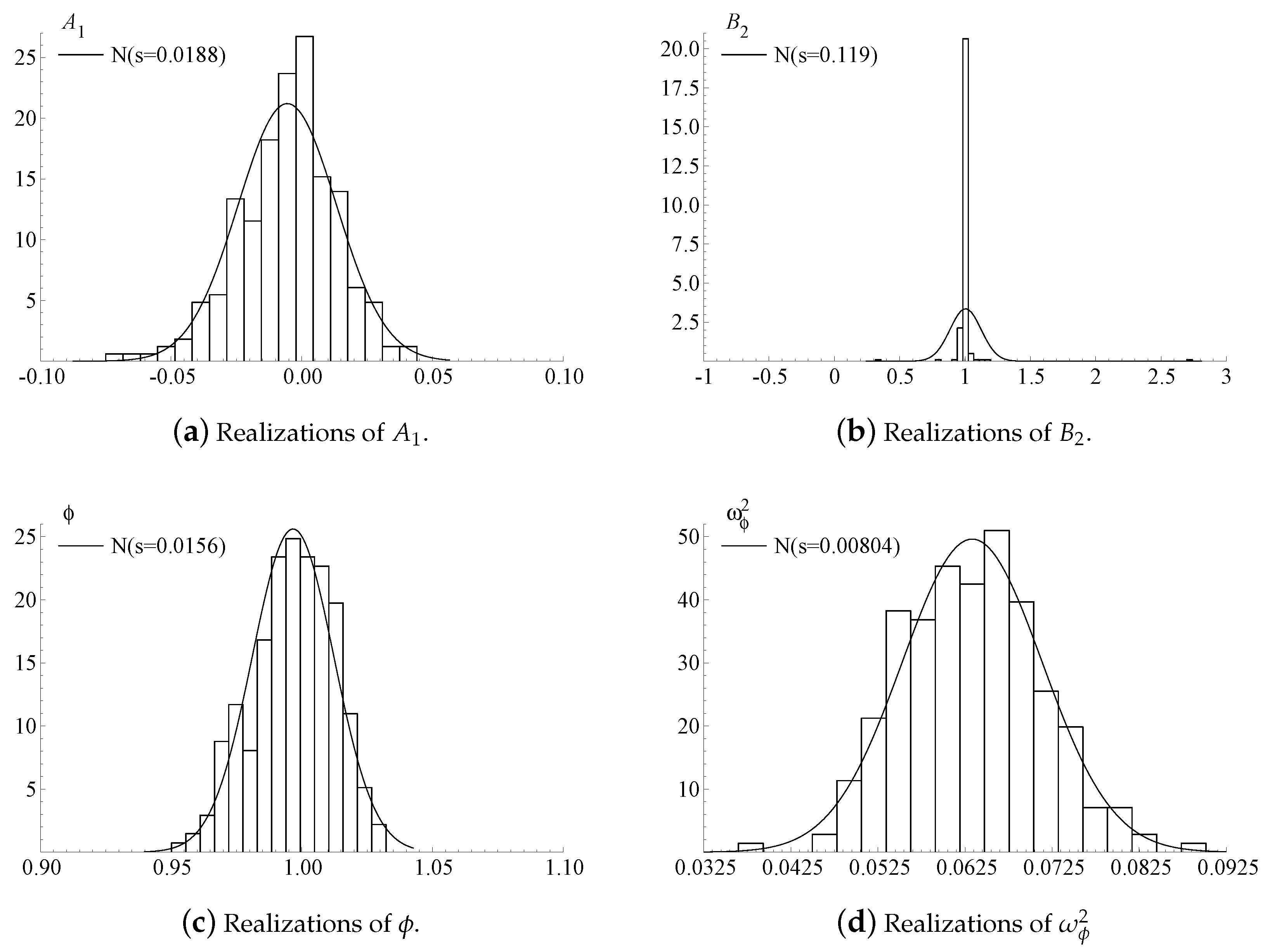
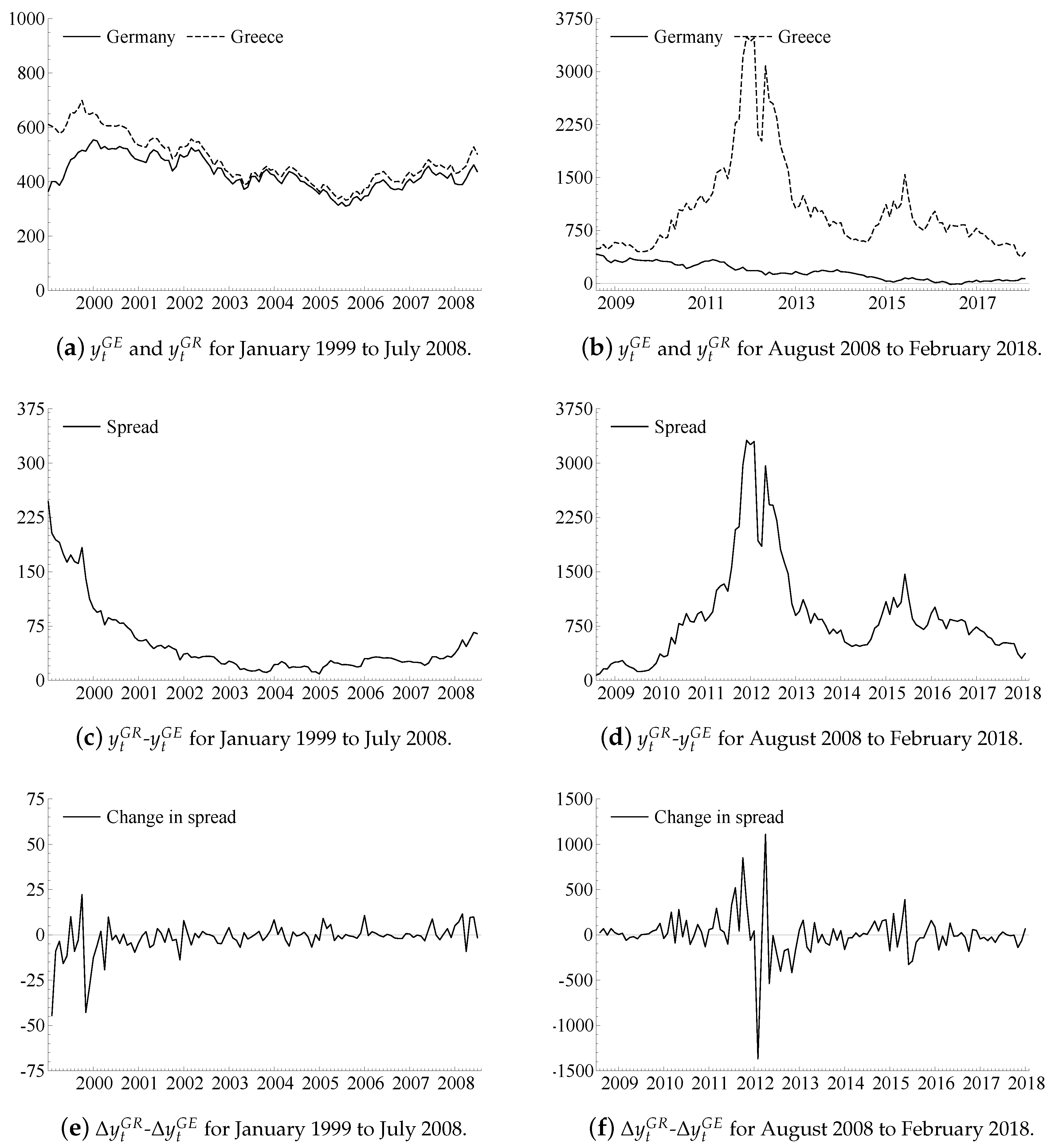
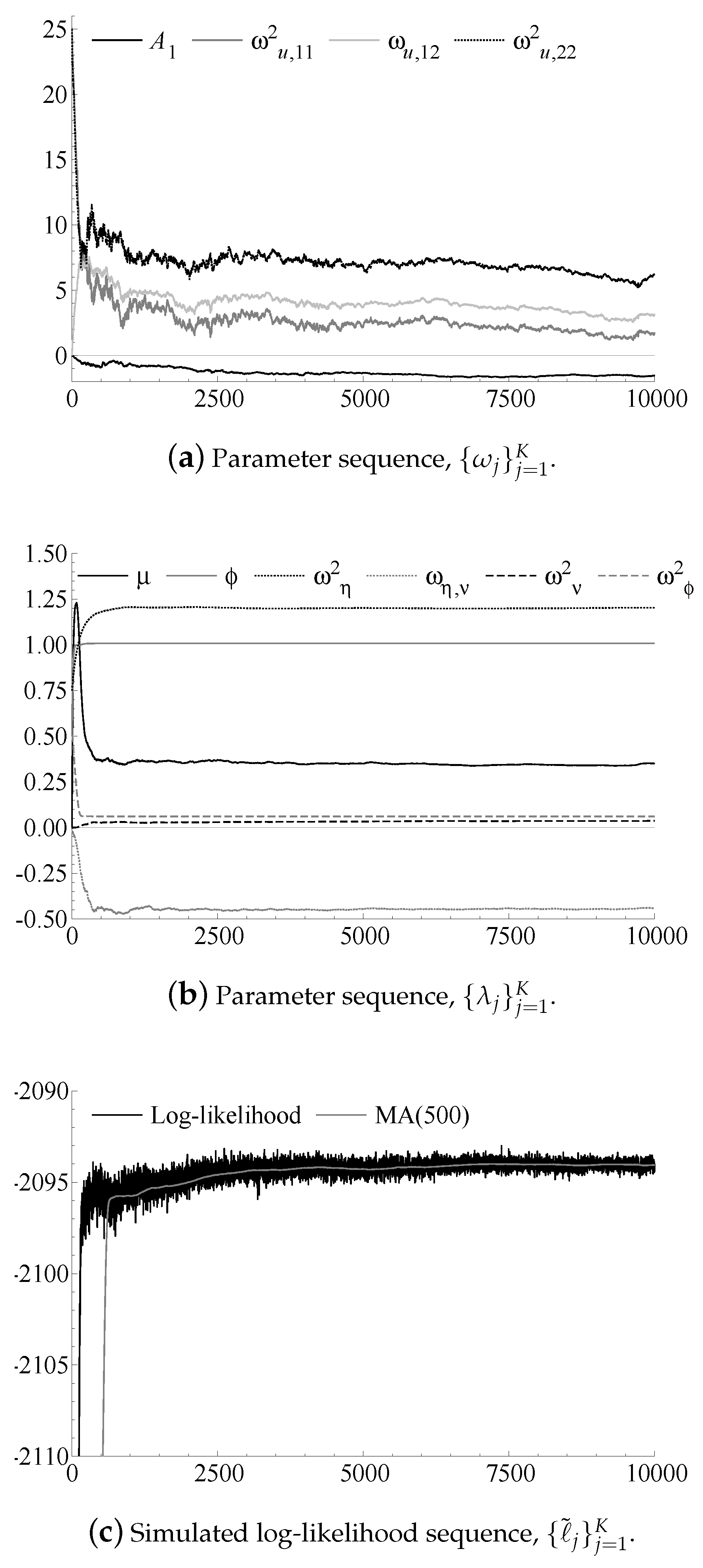
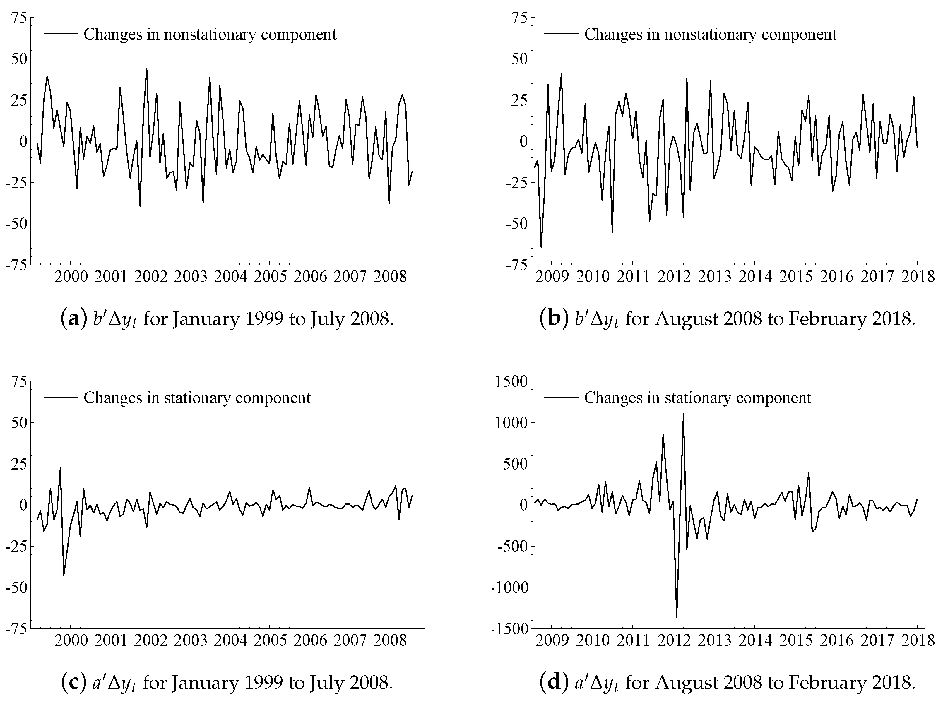
Table 1.
Approximate ML estimate, .
| Parameter | Estimate | Std.err. | Parameter | Estimate | Std.err. |
|---|---|---|---|---|---|
| - | |||||
| - | |||||
| - | |||||
Note: The approximate log-likelihood is . The approximate ML estimate has been obtained by running Algorithm 2 for iterations with the particle count increasing to particles, as described in the main text. The standard errors are based on the inverse of the approximate observed Information matrix computed with particles.
Table 2.
Model diagnostics.
| Univariate tests for AR 1-2: | |||
| Multivariate test for AR 1-2: | |||
| Univariate tests for ARCH: | |||
Note: The approximate normalized one-step prediction errors have been computed with particles for the approximate ML estimate , cf. Table 1.
© 2018 by the author. Licensee MDPI, Basel, Switzerland. This article is an open access article distributed under the terms and conditions of the Creative Commons Attribution (CC BY) license (http://creativecommons.org/licenses/by/4.0/).
Share and Cite
MDPI and ACS Style
Hetland, A. The Stochastic Stationary Root Model. Econometrics 2018, 6, 39. https://0-doi-org.brum.beds.ac.uk/10.3390/econometrics6030039
AMA Style
Hetland A. The Stochastic Stationary Root Model. Econometrics. 2018; 6(3):39. https://0-doi-org.brum.beds.ac.uk/10.3390/econometrics6030039
Chicago/Turabian StyleHetland, Andreas. 2018. "The Stochastic Stationary Root Model" Econometrics 6, no. 3: 39. https://0-doi-org.brum.beds.ac.uk/10.3390/econometrics6030039
Note that from the first issue of 2016, this journal uses article numbers instead of page numbers. See further details here.