Interval Estimation of Value-at-Risk Based on Nonparametric Models

Abstract

Value-at-Risk (VaR) has become the most important benchmark for measuring risk in portfolios of different types of financial instruments. However, as reported by many authors, estimating VaR is subject to a high level of uncertainty. One of the sources of uncertainty stems from the dependence of the VaR estimation on the choice of the computation method. As we show in our experiment, the lower the number of samples, the higher this dependence. In this paper, we propose a new nonparametric approach called maxitive kernel estimation of the VaR. This estimation is based on a coherent extension of the kernel-based estimation of the cumulative distribution function to convex sets of kernel. We thus obtain a convex set of VaR estimates gathering all the conventional estimates based on a kernel belonging to the above considered convex set. We illustrate this method in an empirical application to daily stock returns. We compare the approach we propose to other parametric and nonparametric approaches. In our experiment, we show that the interval-valued estimate of the VaR we obtain is likely to lead to more careful decision, i.e., decisions that cannot be biased by an arbitrary choice of the computation method. In fact, the imprecision of the obtained interval-valued estimate is likely to be representative of the uncertainty in VaR estimate.

1. Introduction

Controlling financial risk is an important issue for financial institutions. For the necessity of risk management, the first task is to measure risk. Value-at-Risk (VaR) is probably the most widely used risk measurement in financial institutions. It has made its way into the Basel II Capital-Adequacy framework. VaR is an estimate of the largest loss over a specified time horizon at a particular probability level. For example, if the daily VaR of an investment portfolio is $10 million with a $95\%$ confidence level, this means that we can be $95\%$ confident that the portfolio will not lose more than $10 million over the next day. In a more formal way, the VaR of a portfolio at a probability level $\alpha$ can be defined as McNeil et al. (2005, p. 38).

$${\mathrm{VaR}}_{\alpha }=inf\{x,F_X(x)=P(X\le x)\ge \alpha \}=F_X^{-1}(\alpha ),$$

(1)

where X is a random variable representing daily percent return for a total stock index with Cumulative Distribution Function (CDF) $F_X$. As McNeil et al. (2005) point out, VaR is simply a quantile of the corresponding loss distribution, which makes its computation easy. Various methods have been proposed in the relevant literature to compute the VaR. Each method differs in the methodology used, the hypotheses, and the way the models are implemented. A highly questionable fact is that each method leads to different results. Thus the choice of computational method is likely to have a large impact on the way a financial institution manages its credit portfolio.

The most commonly used approach is the nonparametric Historical Simulation (HS) method described in Linsmeier and Pearson (1997). It is based on the empirical CDF of the historically simulated returns by attributing an equal probability weight to each day’s return. The HS approach is easy to implement but suffers from two major drawbacks: First, the success of the approach depends on the ability to collect a large series of data; second, this is an unconditional model and thus we need a number of extreme scenarios in the historical record to provide more informative estimates of the tail of the loss distribution McNeil et al. (2005). Moreover, estimates of extreme quantiles are inefficient since extrapolation beyond past observations is impossible. To avoid these drawbacks, several parametric and nonparametric approaches have been developed. For example, Butler and Schachter (1998) propose the kernel estimators in conjunction with the historical simulation method. Also, Charpentier and Oulidi (2010) calculate the VaR by using several nonparametric estimators based on Beta kernel. This study shows that those estimators improve the efficiency of traditional ones, not only for light tailed, but also heavy tailed distributions.

Numerous recent VaR models are referred to as parametric. From the point of view of the risk manager, estimate VaR assuming normal distribution of asset returns is inappropriate and lead to underestimate the left tail at low probability level. For this reason, most recent research papers deal with going beyond the normal model and attempt to capture the related phenomena of heavy and long tails and asymmetric form of the returns series. EVT (Extreme Value Theory) and the so-called GHYP (Generalized HYPerbolic) distributions are among the most widely used. The main advantage of hypothesizing a GHYP distribution is its ability to account for the statistical properties of financial market data such as volatility clustering, asymmetry and heavy-tail phenomena (see McNeil et al. (2005) for an introduction and Paolella and Polak (2015) for a recent application). Kuester et al. (2006) use an EVT-based approach and focuses on the long tails of the return distribution. Braione and Scholtes (2016) study the performance of forecasting VaR under different parametric distributional assumptions and show the predominance and the predictive ability for the skewed and heavy-tailed distributions in the univariate case. The main drawback of using a parametric model is the high dependency of the obtained method to the hypothesized distribution model. To lower this dependency, some authors have proposed a group of semiparametric methods that are based on extreme value theory. These methods have been successfully used by financial analysts in estimating VaR Danielsson and De Vries (2000). However, all the above mentioned attempts have the common weakness of a low robustness to modelling leading to variations in the VaR estimation. To enable this method to be used in a prudent manner, it would be of instrumental interest to estimate the variation of the computed VaR w.r.t. the modelling. Some attempts have been proposed to achieve such a goal. For example, Butler and Schachter (1998) propose a method to measure the precision of a VaR estimate. Jorion (1996) suggests that VaR always be reported with confidence intervals and shows that it is possible to improve the efficiency of VaR estimates using their standard errors. Kupiec (1995) proposes a method for quantifying the uncertainty, in the estimated VaR, induced by the fact that the return distribution is unknown. Pritsker (1997) proposes to estimate a standard error by using a Monte Carlo VaR analysis.

In this paper, we propose a completely new approach to estimate the variations in the VaR induced by choosing a particular model in a kernel-based approach. The idea is that an estimate of the CDF of the daily percent return can be used to compute the VaR as suggested by Equation (1). Such an estimate can be obtained by using a kernel-based approach Silvermann (1986). In Kernel Density Estimation (KDE), the role of the kernel is to achieve an interpolation to lower the impact of sampling on the obtained estimation. Roughly speaking, it smoothes the empirical CDF. However, as in the above mentioned methods, there is a systematic bias induced by the choice of the kernel used to estimate the CDF. Our proposal is to focus on the new nonparametric approach developed by Loquin and Strauss (2008a) to estimate the CDF. This approach makes use of the ability of a new kind of interpolating kernel, called maxitive kernel, to represent a convex set of conventional kernels—that we call summative kernels Loquin and Strauss (2008b). Within this approach, the estimate of the CDF is interval-valued. Such an interval-valued estimate of the CDF, also called a p-box Destercke et al. (2007), is the convex set of all the CDF that would have been computed by using the convex set of conventional summative kernel represented by the maxitive kernel. We show that this approach can advantageously be used to compute with accuracy the corresponding convex set of kernel-based VaR estimates. This approach has advantages over Monte Carlo based approaches since its complexity is comparable to that of classical kernel estimation. Moreover, within this approach the bounds are exact while Monte Carlo approaches provide an inner estimation of those bounds.

This paper is structured as follows. Section 2 reviews some nonparametric and parametric approaches and bootstrap methods used to compute the confidence interval of VaR. In Section 3, we introduce the empirical distribution function and the kernel cumulative estimator based on summative kernel. We define in Section 4 the maxitive kernel, which forms the basis of our approach, and it is shown how an interval-valued estimation of VaR, based on maxtive kernel, can be derived that has relevant properties in this context. Section 5 presents and discusses our empirical findings. Firstly, we show how the choice of kernel function affects the VaR estimates. Secondly, we investigate the performance of the interval-valued proposed in this paper by comparing it to three very competitive approaches: The simple Normal VaR, the HS VaR, and the GHYP VaR. Finally, Section 6 concludes this paper with some further remarks.

Throughout this paper, we consider that the observations belong to a convex and compact subset (universe) $\Omega$ of $\mathrm{I}\mathrm{R}$, called the reference set. $\mathcal{P}(\Omega )$ is the collection of all measurable subsets of $\Omega$. It naturally contains the empty set and is closed under complementation and countable unions. Then $(\Omega ,\mathcal{P}(\Omega ))$ is a measurable space. Let $L(\Omega )$ be the set of functions defined on $\Omega$ with values in $\mathrm{I}\mathrm{R}$.

2. A Review of Some Statistical Approaches and Nonparametric Bootstrap Methods

2.1. Historical Simulation

The HS method calculates the Value-at-Risk using real historical data of asset returns and captures the non-normal distribution of the returns. HS is a nonparametric method because it doesn’t make a specific assumption about distribution of returns. However HS method assumes that the distribution of past returns is a good and complete representation of expected future returns.

The VaR with $\alpha \%$ of probability level is calculated as the $\alpha \%$ percentile of the sorted data return values. For example, with a returns data with 1000 observations, the $1\%$ VaR estimate is simply the negative of the 10^th sample order statistic. This HS VaR can be defined as follows:

$${\mathrm{VaR}}_{\alpha }=\mathrm{percentile}\left({\{r_t\}}_{t=1}^T,\alpha \%\right),$$

where $r_t$ is the asset return at time t.

2.2. GHYP Parametric Distribution

The generalized hyperbolic distribution (GHYP) was introduced by Barndorff-Nielsen (1978) to fit financial returns. The GHYP is an asymmetric heavy-tailed distribution that can account for the extreme events and cater for skewness embedded in the data. It has since been applied in diverse disciplines such as physics, biology, financial mathematics (see Eberlein and Keller (1995); Sørensen and Bibby (1997); Paolella (2007, chp. 9)).

The probability density function (pdf) of univariate GHYP distribution with the parameterization of Eberlein et al. (1998) is given, for $x\in \mathbb{R}$, by:

$$f_{GHD}(x;\lambda ,\chi ,\psi ,\mu ,{\sigma }^2,\gamma )=a{K}_{\lambda -1/2}\left(\sqrt{\left(\chi +\frac{{(x-\mu )}^2}{{\sigma }^2}\right)\left(\psi +\frac{{\gamma }^2}{{\sigma }^2}\right)}\right)exp\left(\gamma \frac{(x-\mu )}{{\sigma }^2}\right){\left((\chi +\frac{{(x-\mu )}^2}{{\sigma }^2})(\psi +\frac{{\gamma }^2}{{\sigma }^2})\right)}^{\lambda /2-1/4},$$

with the normalizing constant

$$a=\frac{{(\chi \psi )}^{-\lambda /2}{\psi }^{\lambda }{(\psi +\frac{{\gamma }^2}{{\sigma }^2})}^{1/2-\lambda }}{{(2\pi )}^{1/2}\sigma K_{\lambda }(\sqrt{\chi \psi })},$$

where

(a)

$K_{\lambda }$ denotes a modified Bessel function of the third kind with index $\lambda$.

(b)

$\lambda$ defines the subclasses of GHYP and is related to the fail flatness.

(c)

$\chi$ and $\psi$ determine the distribution shape; in general, the larger those parameters are, the closer the distribution is to the normal distribution.

(d)

$\mu$ is the location parameter.

(e)

$\sigma$ is the dispersion parameter (standard deviation)

(f)

$\gamma$ is the skewness parameter (if $\gamma =0$, the distribution reduces to the symmetric generalized hyperbolic distribution).

The GHYP family contains many special cases known under special names, listed as follows:

• Hyperbolic Distribution (HYP)
  If $\lambda =1$, we get the hyperbolic distribution. However, HYP distribution is characterized by having a hyperbolic log-density function whereas the logdensity for the normal distribution is a parabola. Thus, one may expect the HYP distribution to be coherent alternatives for heavy tailed data.
• Normal Inverse Gaussian (NIG) Distribution
  If $\lambda =-\frac{1}{2}$, then the distribution is known as normal inverse gaussian (NIG). NIG distribution is also widely used in financial modeling.
• Variance Gamma (VG) Distribution
  If $\lambda >0$ and $\chi =0$, then we obtain the limiting case which is known as variance gamma (VG) distribution.
• The Skewed Student’s -Distribution (St)
  When $\lambda <0$ and $\chi =0$ we get another limiting case called the generalized hyperbolic skew student’s t distribution because it generalizes the usual Student t distribution, obtained from the skewed-t by setting the skewness parameter $\gamma =0$.

In order to estimate the unknown parameters $(\lambda ,\chi ,\psi ,\mu ,{\sigma }^2,\gamma )$, one can use the maximum likelihood (ML) with numerical optimization method (EM-based algorithm).

2.3. Nonparametric Bootstrap Approach

The bootstrap method is used in an important number of statistics topics based on building a sampling distribution for a statistic by resampling from the data at hand. The term bootstrap was coined by Efron (1979), and is an allusion to the expression pulling oneself up by one’s bootstraps—in this case, using the sample data as a population from which repeated samples are drawn Fox (2002). The nonparametric bootstrap allows us to empirically estimate the sampling distribution of a statistic $\theta$—such as a mean, median, standard deviation, or quantile (VaR)—or an estimator $\widehat{\theta }$ without making assumptions about the form of the population, and without deriving the sampling distribution explicitly. The basic idea of the nonparametric bootstrap is as follows: Assuming a data set $\mathcal{S}=(x_1,\cdots ,x_n)$ is available. We draw a sample of size n from among the elements of $\mathcal{S}$, sampling with replacement. This result is called bootstrap sample${\mathcal{S}}_1^{★}=(x_{11}^{★},\cdots ,x_{1n}^{★})$. We repeat this procedure a large number of times, B, selecting many bootstrap samples; the $bth$ such bootstrap sample is denoted ${\mathcal{S}}_b^{★}=\{x_{b1}^{★},\cdots ,x_{bn}^{★}\}$. Next, we compute the statistic $\theta$ for each of the bootstrap samples; that is ${\theta }_b^{★}=t(x_b^{★})$, with t denoting some function, that we can use to estimate from data. Then the distribution of ${\theta }_b^{★}$ around the original estimate $\theta$ is analogous to the sampling distribution of the estimator $\theta$ around the population parameter. The variance is estimated by the sample variance (but for the bootstrap sample of $\widehat{\theta }$) and the bias is estimated by the difference between the average of the bootstrap sample and the original $\widehat{\theta }$. Then, the bootstrap estimates of bias and variance are given approximately by:

$$\mathrm{Bias}({\widehat{\theta }}^{★})\approx \frac{1}{B}\sum _{b=1}^B{\widehat{\theta }}_i^{★}-\widehat{\theta }={\widehat{\theta }}^{★}-\widehat{\theta }\mathrm{and}var({\widehat{\theta }}^{★})\approx \frac{1}{B-1}\sum _{b=1}^B{({\widehat{\theta }}_i^{★}-{\widehat{\theta }}^{★})}^2.$$

There are various methods for constructing bootstrap confidence intervals. The normal-theory interval assumes that the distribution of $\widehat{\theta }$ is normally distributed (which is often approximately the case for statistics in sufficiently large samples), and uses the bootstrap estimate of sampling variance, and perhaps of bias, to construct a $100(1-\alpha )$-percent confidence interval of the form:

$$\left[(\widehat{\theta }-{\widehat{\theta }}^{★})-z_{1-\frac{\alpha }{2}}se({\theta }^{★}),(\widehat{\theta }-{\widehat{\theta }}^{★})+z_{1-\frac{\alpha }{2}}se({\widehat{\theta }}^{★})\right],$$

where $se({\widehat{\theta }}^{★})=\sqrt{var({\widehat{\theta }}^{★})}$ is the bootstrap estimate of the standard error of $\widehat{\theta }$, and $z_{1-\frac{\alpha }{2}}$ is the $1-\frac{\alpha }{2}$ quantile of the standard-normal distribution (e.g., $1.96$ for a 95-percent confidence interval, where $\alpha =0.05$).

We can also estimate confidence intervals using percentiles of the sample distribution: The upper and lower bounds of the confidence interval would be given by the percentile points (or quantiles) of the sample distribution of parameter estimates. This alternative approach, called the bootstrap percentile interval, is to use the empirical quantiles of ${\theta }_b^{★}$ to form a confidence interval $[{\theta }_{(\mathrm{lo})}^{★},{\theta }_{(\mathrm{up})}^{★}]$, where ${\theta }_{(1)}^{★},\cdots ,{\theta }_{(\mathrm{r})}^{★}$ are the ordered bootstrap replicates of the statistic; lo = $[(r+1)\alpha /2]$; up = $[(r+1)(1-\alpha /2)]$; and $[·]$ is the nearest integer function. This basic percentile interval approach is limited itself, particularly if parameter estimators are biased Dowd (2005). It is therefore often better to use the bias-corrected, accelerated (or ${\mathrm{BC}}_a$) percentile intervals. In order ton find the ${\mathrm{BC}}_a$, we firstly calculate $z={\mathsf{\Phi }}^{-1}\rho$, where ${\mathsf{\Phi }}^{-1}(·)$ is the standard-normal quantile function, and $\rho =\frac{{\sum }_{b=1}^r({\theta }_b^{★}\le \theta )}{r+1}$ is the adjust proportion of bootstrap replicates at or below the original-sample estimate $\theta$. If the bootstrap sampling distribution is symmetric, and if $\theta$ is unbiased, then this proportion will be close to $0.5$, and z will be close to 0. Now, let ${\theta }_{(-i)}$ be the value of $\theta$ produced when the $ith$ observation is deleted from the sample there are n of these quantities. Let $\overline{\theta }=\frac{1}{n}{\sum }_{i=1}^n{\theta }_{(-i)}$ be the average of the ${\theta }_{(-i)}$. We calculate

$$\beta =\frac{{\displaystyle \sum _{i=1}^n{\left({\theta }_{(-i)}-\overline{\theta }\right)}^3}}{{\displaystyle 6{\left[\sum _{i=1}^n\left({\theta }_{(-i)}-{\overline{\theta }}^2\right)\right]}^{\frac{3}{2}}}}.$$

We calculate

$${\beta }_1=\mathsf{\Phi }\left[z+\frac{z-z_{1-\frac{\alpha }{2}}}{1-\beta (z-z_{1-\frac{\alpha }{2}})}\right]\mathrm{and}{\beta }_2=\mathsf{\Phi }\left[z+\frac{z+z_{1-\frac{\alpha }{2}}}{1-\beta (z+z_{1-\frac{\alpha }{2}})}\right],$$

where $\mathsf{\Phi }(·)$ is the standard-normal cumulative distribution function. The values ${\beta }_1$ and ${\beta }_2$ are used to locate the endpoints of the corrected percentile confidence interval: $[{\theta }_{({\mathrm{lo}}^{★})}^{★},{\theta }_{({\mathrm{up}}^{★})}^{★}]$, where ${\mathrm{lo}}^{★}=[r{\beta }_1]$ and ${\mathrm{up}}^{★}=[r{\beta }_2]$. When $\beta$ and z are both 0, ${\beta }_1=\mathsf{\Phi }(-z_{1-\frac{\alpha }{2}})=\mathsf{\Phi }(z_{\frac{\alpha }{2}})=\frac{\alpha }{2}$ and ${\beta }_2=\mathsf{\Phi }(z_{1-\frac{\alpha }{2}})=1-\frac{\alpha }{2}$, which corresponds to the (uncorrected) percentile interval.

For more background on the bootstrap approach and a broader array of applications see Efron and Tibshirani (1993); Davison and Hinkley (1997).

The bootstrap approach can be used to estimate the Value-at-Risk (VaR) and a confidence intervals for VaR. A resampling method based on the bootstrap and a bias-correction to improving the Value-at-Risk (VaR) forecasting ability of the normal-GARCH model has been developed in Hartz et al. (2006). As mentioned in Dowd (2005), if we have a data set of n observations, we create a new data set by taking n drawings, each taken from the whole of the original data set. Each new data set created in this way gives us a new VaR estimate. We then create a large number of such data sets and estimate the VaR of each. The resulting VaR distribution function enables us to obtain estimates of the confidence interval for our VaR. For estimate confidence intervals using a bootstrap approach, we produce a bootstrapped histogram of resample-based VaR estimates, and then read the confidence interval from the quantiles of this histogram. A very good discussion on this and other improvements can be seen in Dowd (2005, chp. 4). In Section 5.3, we use the bias corrected method to estimate the confidence interval of VaR obtained form HS, Normal and GHYP distribution. The purpose of this simulation exercise is to compare these methodologies with our maxitive kernel approach, in order to identify that our interval-valued estimation of VaR perform properly.

3. Summative Kernels

3.1. Summative Kernels and Probability Distributions

Kernels are used in signal processing and nonparametric statistics to define a weighted neighborhood around a location $u\in \Omega$. In kernel regression, it is used to estimate the conditional expectation of a random variable (see e.g., Silvermann 1986; Wand and Jones 1995).

Definition 1.

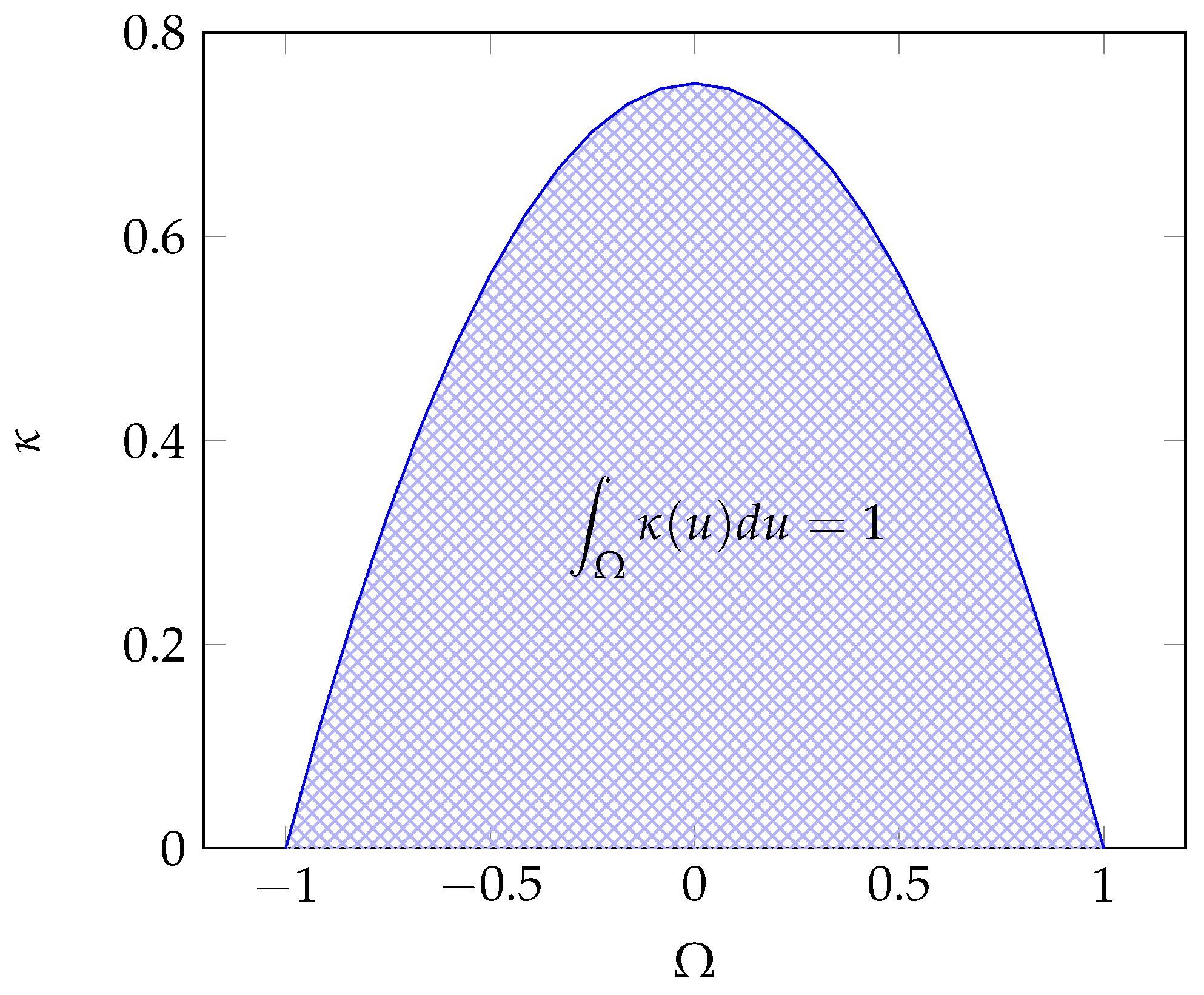
A summative kernel—or conventional kernel—is a positive function $\kappa :\Omega ⟶\mathrm{I}{\mathrm{R}}^{+}$ that verifies the summativity property

$${\int }_{\Omega }\kappa (u)du=1.$$

From a basic summative kernel $\kappa$, we can define a summative kernel ${\kappa }_{\Delta }^x$ translated in $x\in \Omega$ and dilated with a bandwidth $\Delta >0$ by

$${\displaystyle \forall u\in \Omega ,{\kappa }_{\Delta }^x(u)=\frac{1}{\Delta }\kappa (\frac{u-x}{\Delta }).}$$

By convention, $\kappa (u)={\kappa }_1^0(u)$.

The most used summative kernels in functional estimation are usually unimodal, symmetric, and centered (i.e., defining a weighted neighborhood around the origin). When $\kappa (u)$ is symmetric and unimodal function, then the following conditions are fulfilled

$${\int }_{\Omega }u\kappa (u)du=0\mathrm{and}{\int }_{\Omega }{u}^2\kappa (u)du=c>0.$$

For example, the Epanechnikov kernel proposed by Epanechnikov (1969) illustrated in Figure 1 is defined by

$$\kappa (u)=\left\{\begin{array}{cc}\frac{3}{4}\left(1-u^2\right)\hfill & \mathrm{if}\left|u\right|\le 1,\hfill \\ 0\hfill & \mathrm{otherwise}.\hfill \end{array}\right.$$

(2)

In the following, $\mathcal{K}(\Omega )$ represents the set of unimodal, symmetric, and centered kernels. A summative kernel $\kappa$ can be seen as a probability distribution inducing a probability measure $P_{\kappa }:\mathcal{P}(\Omega )\to [0,1]$ on the measurable space ($\Omega ,\mathcal{P}(\Omega )$). $P_{\kappa }$ is defined by

$$\forall A\subseteq \Omega ,P_{\kappa }(A)={\int }_A\kappa (u)du.$$

Considering the summative kernel $\kappa$, we can define what we call the summative expectation as follows:

Definition 2.

Let s be a function of $L(\Omega )$ and let κ be a summative kernel of $\mathcal{K}(\Omega )$. The summative expectation of s, in the neighborhood defined by κ, is the classical expectation of s w.r.t. $P_{\kappa }$:

$${\mathbb{E}}_{\kappa }(s)={\int }_{\Omega }sd{P}_{\kappa }={\int }_{\Omega }s(u)\kappa (u)du,$$

(3)

since $d{P}_{\kappa }=\kappa (u)du$.

3.2. Empirical Distribution Function

Let $(x_1,\cdots ,x_n)$ be a finite set of observations of n random variables $(X_1,\cdots ,X_n)$ i.i.d with unknown pdf f and CDF F. One can estimate F by the empirical CDF $F_n$ defined by

$$F_n(x)=\frac{1}{n}\sum _{i=1}^{n}1\mathrm{l}(x_i\le x),$$

(4)

where $1\mathrm{l}$ is the indicator function, namely $1\mathrm{l}(x_i\le x)=1$ if $x_i\le x$ and zero otherwise. Obviously $1\mathrm{l}(x_i\le x)=1$ with probability $P(x_i\le x)=F(x)$, and $1\mathrm{l}(x_i\le x)=0$ with probability $P(x_i>x)=1-F(x)$. Then $1\mathrm{l}(x_i\le x)$ is a Bernoulli random variable with success probability $F(x)$. Since the $x_i$ are independent, so are the $1\mathrm{l}(x_i\le x)$. Thus $Y_n={\sum }_{i=1}^{n}1\mathrm{l}(x_i\le x)$ (a sum of independent $\mathcal{B}er\{F(x)\}$ random variables) is a $\mathcal{B}in\{n,F(x)\}$ random variable, and

$$F_n(x)\sim \frac{1}{n}\mathcal{B}in\{n,F(x)\}.$$

Then $\forall x\in \Omega$,

$$\mathbb{E}(F_n(x))=F(x)\mathrm{and}Var(F_n(x))=\frac{F(x)(1-F(x))}{n}.$$

This implies that the empirical CDF is convergent in probability to the true CDF:

$$\forall x\in \Omega ,F_n(x)\stackrel{\mathbb{P}}{\to }F(x).$$

Thus the empirical estimate of Value-at-Risk

$${\mathrm{VaR}}_{\alpha ,n}=inf\left\{x,F_n(x)=P(X\le x)\ge \alpha \right\},$$

(5)

converges towards the true ${\mathrm{VaR}}_{\alpha }$.

3.3. Summative Kernel Cumulative Estimator

The empirical distribution function (Equation (4)) is not smooth as it jumps by $\frac{1}{n}$ at each point $x_i$ ($i=1\cdots n$). A kernel estimator of the CDF, introduced by authors such as Nadaraya (1964); and Watson and Leadbetter (1964), is a smoothed version of the empirical distribution estimator. Such an estimator arises as an integral of the Parzen-Rosenblatt kernel density estimator (see Rosenblatt 1956; Parzen 1962).

Definition 3.

The summative-kernel cumulative estimator of the CDF (also called the Parzen-Rosenblatt kernel cumulative estimator), based on the summative kernel κ is given, in each point $x\in \Omega$, by

$${\widehat{F}}_{\kappa }^n(x)=\frac{1}{n}\sum _{i=1}^n\mathsf{\Gamma }\left(x-x_i\right),$$

(6)

where ${\displaystyle \mathsf{\Gamma }(x)={\int }_{-\infty }^x\kappa (u)du}$.

Let $\kappa \in \mathcal{K}(\Omega )$ be a summative kernel function of the second order with support $[-1,1]$, the function $\mathsf{\Gamma }(u)$ verifies the following properties

$$\mathsf{\Gamma }(u)=\left\{\begin{array}{cc}0\hfill & \mathrm{if}u\in ]-\infty ,-1],\hfill \\ 1\hfill & \mathrm{if}u\in ]1,\infty ].\hfill \end{array}\right.$$

$$\left\{\begin{array}{c}{\displaystyle {\int }_{-1}^1{\mathsf{\Gamma }}^2(u)du\le {\int }_{-1}^1\mathsf{\Gamma }(u)du=1,}\hfill \\ {\displaystyle {\int }_{-1}^1\mathsf{\Gamma }(u)\kappa (u)du=\frac{1}{2},}\hfill \\ {\displaystyle {\int }_{-1}^{1}u\mathsf{\Gamma }(u)\kappa (u)du=\frac{1}{2}\left(1-{\int }_{-1}^1{\mathsf{\Gamma }}^2(u)du\right).}\hfill \end{array}\right.$$

Note that if $\kappa$ is the pdf of a probability measure $P_{\kappa }$, then $\mathsf{\Gamma }$ is the cumulative distribution function of $P_{\kappa }$. For example, $\kappa$ being the Epanechnikov kernel defined by (2), the function $\mathsf{\Gamma }$, depicted in Figure 2, has the following expression:

$$\mathsf{\Gamma }(u)=\left\{\begin{array}{cc}0\hfill & \mathrm{if}u\le -1,\hfill \\ {\displaystyle -\frac{1}{4}{u}^3+\frac{3}{4}u+\frac{1}{2}}\hfill & \mathrm{if}\left|u\right|\le 1,\hfill \\ 1\hfill & \mathrm{if}u\ge 1.\hfill \end{array}\right.$$

(7)

Let $\kappa \in \mathcal{K}(\Omega )$ be a summative kernel with support $[-1,1]$, for a fixed x, the bias and the variance of ${\widehat{F}}_{\kappa }^n(x)$ are given by

$$\mathbb{E}\left({\widehat{F}}_{\kappa }^n(x)\right)-F(x)=\frac{{\Delta }^2}{2}{f}^{\prime }(x){\int }_{\Omega }{u}^2\kappa (u)du+o({\Delta }^2),$$

$$var({\widehat{F}}_{\kappa }^n(x))=\frac{1}{n}\left\{F(x)\left(1-F(x)\right)+\Delta f(x)\left({\int }_{-1}^{+1}{\kappa }^2(u)du-1\right)+o(\Delta )\right\}.$$

Some theoretical properties of the estimator ${\widehat{F}}_{\kappa }^n$ have been investigated, among others, by Winter (1973); Winter (1979); Sarda (1993); Yamato (1973); and Jones (1990). Some properties have long been known, e.g., the uniform convergence of ${\widehat{F}}_{\kappa }^n$ towads F when the pdf $f=dF$ is continuous Nadaraya (1964); and Yamato (1973) or without conditions on f Singh et al. (1983). The asymptotic expression of the Mean Integrated Squared Error (MISE) (i.e., ${\int }_{\Omega }{({\widehat{F}}_{\kappa }^n(x)-F(x)dx)}^2$ has been studied in Swanepoel (1988). For a continuous pdf f, it has been proved that the best kernel is the uniform kernel of bandwidth $\Delta >0$ defined by $\kappa (u)=\frac{1}{2\Delta }{1\mathrm{l}}_{[-\Delta ,\Delta ]}(u)$ and for a discontinuous function f, in a finite number of points, the best kernel is the exponential kernel of bandwidth $\Delta >0$ defined by $\kappa (u)=\frac{\Delta }{2}{e}^{-\Delta \left|u\right|}$.

The method of choosing the optimal value of bandwidth in kernel estimation of the cumulative distribution function is of crucial interest. Many procedures—such as plug-in and cross validation—have been proposed in the relevant literature (see e.g., Sarda 1993; Polansky and Baker 2000; Altman and Leger 1995) to choose (estimate) the optimal bandwidth for estimating the CDF of the random process underlying a sample. As mentioned in Quintela Del Rio and Estevez-Perez (2013), the Polansky and Baker plug-in bandwidth is given by

$${\Delta }_{\mathrm{PB}}={\left(\frac{\zeta (\kappa )}{-n{\xi }_2^2(\kappa ){\widehat{V}}_2(g_2)}\right)}^{1/3},$$

where

$${\xi }_2(\kappa )={\int }_{\Omega }{u}^2\kappa (u)du;\zeta (\kappa )=2{\int }_{\Omega }u\kappa (u)\mathsf{\Gamma }(u)du,$$

$${\widehat{V}}_r(g)=\frac{1}{n^2{g}^{r+1}}\sum _{i=1}^n\sum _{j=1}^n{H}^{(r)}\left(\frac{x_i-x_j}{g}\right)$$

estimates

$$V_r={\int }_{\Omega }{f}^{(r)}(u)f(u)du,$$

where $r\ge 2$ is an even integer and

$$g_2={\left(\frac{2H^{(2)}(0)}{-n{\xi }_2^2(H)V_4}\right)}^{1/5}.$$

The kernel function H is not necessarily equal to $\kappa$. An iterative method for calculating the plug-in bandwidth has been proposed by Polansky and Baker (2000). As mentioned in Quintela Del Rio and Estevez-Perez (2013), the plug-in bandwidth is calculated as follows: let $b>0$ be an integer, firstly, we calculate ${\widehat{V}}_{2b+2}$ using

$${\widehat{V}}_r=\frac{{(-1)}^{r/2}r!}{{(2\widehat{\sigma }(x_i))}^{r+1}(r/2)!{(3.14)}^{1/2}},$$

where $\sigma$ is the standard deviation of the data which can be estimated by $\widehat{\sigma }(x_i)=min\{\widehat{s},\frac{Q_3-Q_1}{1.349}\}$, with $\widehat{s}$ is the sample standard deviation, and $Q_1,Q_3$ denoting the first and third quartile, respectively. Secondly, begin form $j=b$ to $j=1$, we calculate ${\widehat{V}}_{2j}({\widehat{g}}_{2j})$, where

$${\widehat{g}}_{2j}={\left(\frac{2H^{(2j)}(0)}{-n{\xi }_2(H){\widehat{V}}_{2j+2}}\right)}^{1/(2j+3)},$$

with

$${\widehat{V}}_{2j+2}=\left\{\begin{array}{c}{\widehat{V}}_{2b+2},\mathrm{if}j=b,\hfill \\ {\widehat{V}}_{2j+2}({\widehat{g}}_{2j+2}),\mathrm{if}j<b.\hfill \end{array}\right.$$

Thirdly, the plug-in bandwidth is

$${\widehat{\Delta }}_{\mathrm{PB}}={\left(\frac{\zeta (\kappa )}{-n{\xi }_2^2(\kappa ){\widehat{V}}_{2j}({\widehat{g}}_{2j})}\right)}^{1/3}.$$

In practice, for most applications, we consider $b=2$ Quintela Del Rio and Estevez-Perez (2013).

Sarda (1993) introduced a cross-validation method to estimate the optimal bandwidth which minimize the MISE:

$$CV(\Delta )=\sum _{i=1}^n{\left(F_n(x_i)-{\widehat{F}}_{\kappa ;-i}^n(x_i)\right)}^2,$$

where $F_n$ is the empirical distribution function (Equation (4)) and ${\widehat{F}}_{\kappa ;-i}^n$ is the kernel cumulative distribution estimator computed by leaving out $x_i$:

$${\widehat{F}}_{\kappa ;-i}^n(u)=\frac{1}{n-1}\sum _{j\ne i}\mathsf{\Gamma }(u-x_j).$$

Adrian et al. (1998) proposed a modified cross-validation method which minimizes the function

$$CV(\Delta )=\frac{1}{n}\sum _{i=1}^n{\int }_{\Omega }{\left(1\mathrm{l}(u-x_i)-{\widehat{F}}_{\kappa ;-i}^n(u)\right)}^{2}du.$$

For more details about bandwidth selection of summative kernel CDF estimation, we refer our reader to Quintela Del Rio and Estevez-Perez (2013).

Now, if we suppose that all parameters have been chosen appropriately for ${\widehat{F}}_{\kappa }^n$ to be a consistent estimate of the CDF, then a kernel estimator of VaR, denoted ${\widehat{\mathrm{VaR}}}_{\alpha ,\kappa }$, can be easily obtained by inverting the equation ${\widehat{F}}_{\kappa }^n(x)=\alpha$. In that case, ${\widehat{\mathrm{VaR}}}_{\alpha ,\kappa }$ satisfies:

$$\frac{1}{n}\sum _{i=1}^n\mathsf{\Gamma }\left({\widehat{\mathrm{VaR}}}_{\alpha ,\kappa }-x_i\right)=\alpha .$$

(8)

The kernel VaR estimator ${\widehat{\mathrm{VaR}}}_{\alpha ,\kappa }$ can be seen as a smoothed version of the empirical distribution function of VaR (${\mathrm{VaR}}_{\alpha ,n}$) defined by (Equation (5)). For further details about the properties of the kernel VaR estimator (see e.g., Gourieroux et al. 2000; Chen and Tang 2005; Sheather and Marron 1990). However, the validity of such an estimate highly depends on the appropriateness of the chosen kernel and bandwidth. In the next Section, we propose another approach that allows to estimate the dependance of the obtained estimate to the parameters of the method, and therefore to increase the robustness of the decision process based on the data.

4. Maxitive Kernels

4.1. Maxitive Kernels and Possibility Distributions

In many applications the summative kernels and their bandwidth are chosen in a very empirical way. As proposed in Loquin and Strauss (2008b), the empirical character of choosing a kernel could be taken in consideration by taking a family of kernels rather than one kernel. This family of kernels can be represented by using a maxitive kernel.

Definition 4.

A maxitive kernel is a positive function $\pi :\Omega ⟶\left[0,1\right]$ that verifies the following maxitivity property

$$\underset{u\in \Omega }{sup}\pi (u)=1.$$

From a basic maxitive kernel $\pi$, we can define a maxitive kernel ${\pi }_{\Delta }^x$ translated in $x\in \Omega$ and dilated with a bandwidth $\Delta >0$ by

$$\forall u\in \Omega ,{\pi }_{\Delta }^x(u)=\pi \left(\frac{u-x}{\Delta }\right).$$

By convention, $\pi (u)={\pi }_1^0(u)$.

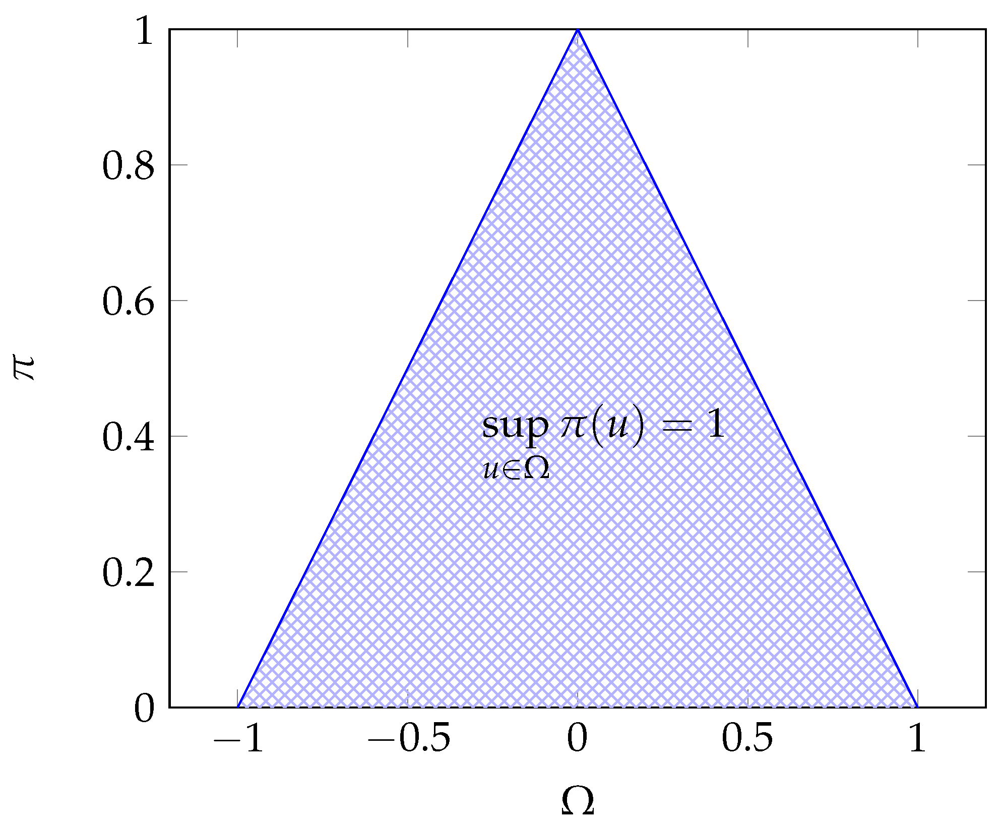
For example, the triangular maxitive kernel proposed in Loquin and Strauss (2008b) illustrated in Figure 3 is defined by

$$\pi (u)=\left\{\begin{array}{cc}1-\left|u\right|\hfill & \mathrm{if}\left|u\right|\le 1,\hfill \\ 0\hfill & \mathrm{otherwise}.\hfill \end{array}\right.$$

(9)

A maxitive kernel can be seen as a possibility distribution Loquin and Strauss (2008b), inducing two dual non-additive confidence measures, a possibility measure ${\Pi }_{\pi }$, and a necessity measure $N_{\pi }$ Dubois and Prade (1988); and De Cooman (1997) defined, $\forall A\subseteq \Omega$, by

$$\begin{array}{cc}\hfill {\Pi }_{\pi }(A)& =\underset{x\in A}{sup}\pi (x)(\mathrm{possibility}),\hfill \\ \hfill N_{\pi }(A)& =1-{\Pi }_{\pi }(A^c)(\mathrm{necessity}),\hfill \end{array}$$

with $A^c$ being the complementary set of A in $\Omega$.

A maxitive kernel $\pi$ is said to dominate a summative kernel $\kappa$ Loquin and Strauss (2008b), if the possibility measure ${\Pi }_{\pi }$ dominates the probability measure $P_{\kappa }$, i.e.,

$$\forall A\subseteq \Omega ,P_{\kappa }(A)\le {\Pi }_{\pi }(A).$$

In that sense, a maxitive kernel defines the convex set of summative kernels it dominates. This set is denoted $\mathcal{M}(\pi )$ and defined by

$$\mathcal{M}(\pi )=\left\{\kappa \in \mathcal{K}(\Omega )/\forall A\subseteq \Omega ,N_{\pi }(A)\le P_{\kappa }(A)\le {\Pi }_{\pi }(A)\right\}.$$

(10)

The specificity of a maxitive kernel $\pi$, defined by its integral, i.e., $Sp(\pi )={\int }_{\Omega }\pi (u)du$, is a measure of the information contained by the possibility measure associated to $\pi$ Loquin and Strauss (2008b). A maxitive kernel ${\pi }_1$ is at least as informative as another one ${\pi }_2$ if $\forall u\in \Omega$, ${\pi }_1(u)\le {\pi }_2(u)$ Dubois (2006). In that case ${\pi }_1$ is at least as specific as ${\pi }_2$. It also characterizes the amount of summative kernels dominated by $\pi$ in the sense that, if $\forall u\in \Omega$, ${\pi }_1(u)\le {\pi }_2(u)$, then $Sp({\pi }_1)\le Sp({\pi }_2)$ and $\mathcal{M}({\pi }_1)\subseteq \mathcal{M}({\pi }_2)$. Moreover, if $\exists u_0\in \Omega$, such that ${\pi }_1(u_0)<{\pi }_2(u_0)$, then $Sp({\pi }_1)<Sp({\pi }_2)$ and $\mathcal{M}({\pi }_1)\subset \mathcal{M}({\pi }_2)$.

In this context, Dubois et al. (2004) proved that the triangular maxitive kernel, defined by (Equation (9)), with a support $[-\Delta ,+\Delta ]$ is the most specific maxitive kernel that dominates all summative symmetric and unimodal kernels whose support belongs to $[-\Delta ,+\Delta ]$.

4.2. Choquet Integrals and Maxitive Expectation

We start with the definition of a capacity or non-additive measure which generalize the notion of additive measure, i.e., probability. The notion of capacity was introduced by Gustave Choquet in 1953 and has played an important role in game theory, fuzzy set theory, Dempster-Shafer theory and many others (see Denneberg 1994; Shafer 1976; Choquet 1953).

Definition 5.

Let $(\Omega ,\mathcal{P}(\Omega ))$ be the measurable space. A capacity ν on $(\Omega ,\mathcal{P}(\Omega ))$ is a set function $\nu :\mathcal{P}(\Omega )\to \left[0,1\right]$ satisfying:

• ν is normalized (i.e., $\nu (⌀)=0$ and $\nu (\Omega )=1)$.
• ν is monotone (i.e., $\forall A,B\in \mathcal{P}(\Omega )$, $A\subseteq B\Rightarrow \nu (A)\le \nu (B))$.

One of the most important concepts closely related to additive measures is integration. It has a natural generalization to non-additive measure theory. Historically the first applied integral with respect to non-additive measures is the Choquet Integral formalized by Gustave Choquet.

Definition 6.

Let $(\Omega ,\mathcal{P}(\Omega ))$ be the measurable space and $\nu :\mathcal{P}(\Omega )\to \left[0,1\right]$ a capacity. Let s be a bounded function of $L(\Omega )$. The continuous Choquet integral of s w.r.t. ν is defined by

$${\mathbb{C}}_{\nu }(s)=C{\int }_{\Omega }sd\nu ={\int }_{-\infty }^0\left(\nu \left(\{u\in \Omega :s(u)\ge z\}\right)-1\right)dz+{\int }_0^{\infty }\nu \left(\{u\in \Omega :s(u)\ge z\}\right)dz,$$

(11)

where the integral on the right hand side is a Riemann integral.

Definition 7.

Let ν be a capacity on $(\Omega ,\mathcal{P}(\Omega ))$ and $x=(x_1,\cdots ,x_n)\in {\Omega }^n$ be a discrete function $[1,\cdots ,n]\to \Omega$ of n samples. The discrete Choquet integral of x w.r.t. ν is defined by:

$${\mathbb{C}}_{\nu }(x)=C{\int }_{\Omega }xd\nu =\sum _{i=1}^n\left(x_{\tau (i)}-x_{\tau (i-1)}\right)\nu (A_{\tau (i)}),$$

(12)

where τ is the permutation on $[1,\cdots ,n]$, such that $x_{\tau (1)}\le \cdots \le x_{\tau (n)}$, $A_{\tau (i)}:=\{\tau (i),\cdots ,\tau (n)\}$ and $x_{\tau (0)}=0$ by convention.

Note that, a probability P being a special case of (additive) capacity, the Choquet integral w.r.t. P coincides with the classical expected value w.r.t. P.

Recall that, if X is a random variable defined on a probability space ($\Omega ,\mathcal{P}(\Omega ),P$), then the classical expected value of X is given by

$${\mathbb{E}}_P(X)={\int }_{\Omega }XdP={\int }_{\Omega }X(u)dP(u),$$

(13)

where $P:\mathcal{P}(\Omega )\to [0,1]$ is a probability measure on the measurable space ($\Omega ,\mathcal{P}(\Omega )$) and the integral is a Lebesgue-Stieltjes integral.

The notion of expectation w.r.t. a summative kernel can be extended to a maxitive kernel, as defined in Loquin and Strauss (2008b).

Definition 8.

Let π be a maxitive kernel and let s be a bounded function of $L(\Omega )$. The expectation of s w.r.t π is defined by:

$${\underline{\overline{\mathbb{E}}}}_{\pi }(s)=\left[{\underline{\mathbb{E}}}_{\pi }(s),{\overline{\mathbb{E}}}_{\pi }(s)\right]=\left[{\mathbb{C}}_{N_{\pi }}(s),{\mathbb{C}}_{{\Pi }_{\pi }}(s)\right],$$

(14)

where ${\Pi }_{\pi }$ (rsp. $N_{\pi }$) is the possibility (rsp. necessity) measure induced by the maxitive kernel π and $\mathbb{C}$ is the Choquet integral.

An important property, that will be used in the sequel, is that the maxitive interval-valued expectation of s w.r.t. $\pi$ is the convex set of all the summative precise-valued expectations w.r.t. all the summative kernels dominated by $\pi$ Loquin and Strauss (2008b).

Property 1.

Let π be a maxitive kernel and let $\mathcal{M}(\pi )$ be the set of the summative kernels it dominates (see Equation (10)). Let s be a bounded function of $L(\Omega )$. We have

$$\forall g\in {\underline{\overline{\mathbb{E}}}}_{\pi }(s),\exists \kappa \in \mathcal{M}(\pi ):{\mathbb{E}}_{\kappa }(s)=g,$$

(15)

and

$$\forall \kappa \in \mathcal{M}(\pi ),{\mathbb{E}}_{\kappa }(s)\in {\underline{\overline{\mathbb{E}}}}_{\pi }(s),$$

(16)

where ${\mathbb{E}}_{\kappa }(s)$ resp. $\left({\underline{\overline{\mathbb{E}}}}_{\pi }(s)\right)$ is the summative (resp. maxitive) expectation of s w.r.t. κ (resp.π).

4.3. Maxitive Kernel Cumulative and VaR Estimator

As mentioned in Loquin and Strauss (2008a) (Theorem 4), the summative kernel cumulative estimator ${\widehat{F}}_{\kappa }^n$, defined by (Equation (3)), in each point $x\in \Omega$, can be written as the summative expectation of the empirical CDF $F_n$, defined by (Equation (4)), in a probabilistic neighborhood defined by the summative kernel $\kappa$ translated in x

$${\widehat{F}}_{\kappa }^n(x)={\mathbb{E}}_{{\kappa }^x}(F_n).$$

(17)

Based on this reformulation, Loquin and Strauss (2008a) propose an extension of the summative kernel estimator of the CDF. This extension called maxitive kernel estimator of the CDF or interval-valued estimation of the CDF.

Definition 9.

Let $F_n$ be the empirical CDF based on the sample $(x_1,\cdots ,x_n)$. Let π be a maxitive kernel and let ${\underline{\overline{\mathbb{E}}}}_{\pi }(·)$ be the maxitive expectation w.r.t. π (Expression (14)). The maxitive kernel cumulative estimator is defined, $\forall x\in \Omega$, by

$${\underline{\overline{F}}}_{\pi }^n(x)=\left[{\underline{F}}_{\pi }^n(x),{\overline{F}}_{\pi }^n(x)\right]={\underline{\overline{\mathbb{E}}}}_{{\pi }^x}(F_n)=\left[{\underline{\mathbb{E}}}_{{\pi }^x}(F_n),{\overline{\mathbb{E}}}_{{\pi }^x}(F_n)\right].$$

(18)

The computation of ${\underline{\overline{F}}}_{\pi }^n$ involves two Choquet integrals. This computation Loquin and Strauss (2008a) is given, for all $x\in \Omega$, by

$$\begin{array}{cc}\hfill {\underline{F}}_{\pi }^n(x)={\underline{\mathbb{E}}}_{{\pi }^x}(F_n)& ={\mathbb{C}}_{N_{{\pi }^x}}(F_n)=\frac{1}{n}\sum _{i=1}^n\left(\left(1-{\pi }^x(x_i)\right)1\mathrm{l}(x_i\le x)\right),\hfill \end{array}$$

(19)

$$\begin{array}{cc}\hfill {\overline{F}}_{\pi }^n(x)={\overline{\mathbb{E}}}_{{\pi }^x}(F_n)& ={\mathbb{C}}_{{\Pi }_{{\pi }^x}}(F_n)=\frac{1}{n}\sum _{i=1}^n\left({\pi }^x(x_i)1\mathrm{l}(x\le x_i)+1\mathrm{l}(x_i\le x)\right).\hfill \end{array}$$

(20)

The estimation of the CDF is usually computed on p regularly spaced points of $\Omega$. Let ${\{y_j\}}_{j\in \{1,\cdots ,p\}}$ be those p points. The algorithm of compute of ${\left\{{\underline{\overline{F}}}_{\pi }^n(y_j)\right\}}_{j\in \{1,\cdots ,p\}}$, in each point ${\{y_j\}}_{j\in \{1,\cdots ,p\}}$ of $\Omega$, is given by Algorithm 1.

Algorithm 1: Computation of ${\left\{\left[{\underline{F}}_{\pi }^n(y_j),{\overline{F}}_{\pi }^n(y_j)\right]\right\}}_{j\in \{1,\cdots ,p\}}$.

The interval-values estimate ${\underline{\overline{F}}}_{\pi }^n$ based on a maxitive kernel $\pi$ (Expression (9)) is the most specific interval containing all summative estimate ${\widehat{F}}_{\kappa }^n$ (Expression (6)) based on a summative kernel $\kappa$ dominated by $\pi$, i.e., such that $\kappa \in \mathcal{M}(\pi )$.

Property 2.

Let π be a maxitive kernel on Ω and $\mathcal{M}(\pi )$ the set of all the summative kernels dominated by π. We have

$$\forall x\in \Omega ,\forall \kappa \in \mathcal{M}(\pi ),{\widehat{F}}_{\kappa }^n(x)\in {\underline{\overline{F}}}_{\pi }^n(x),$$

and

$$\forall g\in {\underline{\overline{F}}}_{\pi }^n(x),\exists \kappa \in \mathcal{M}(\pi ),{\widehat{F}}_{\kappa }^n(x)=g.$$

Notice that, due to Property 2, both ${\overline{F}}_{\pi }$ and ${\underline{F}}_{\pi }$ are also estimates of the sought after CDF. Clearly, ${\underline{F}}_{\pi }^n$ and ${\overline{F}}_{\pi }^n$ are two strictly increasing continuous functions on $\Omega$, and so they both have an inverse. Then, we can infer immediately an maxitive interval-valued estimation of the VaR ${\underline{\overline{\mathrm{VaR}}}}_{\alpha ,\pi }=[{\underline{\mathrm{VaR}}}_{\alpha ,\pi },{\overline{\mathrm{VaR}}}_{\alpha ,\pi }]$:

$$\begin{array}{c}\hfill {\underline{\mathrm{VaR}}}_{\alpha ,\pi }=inf\left\{x,{\underline{F}}_{\pi }(x)=P(X\le x)\ge \alpha \right\}={\underline{F}}_{\pi }^{-1}(\alpha ),\\ \hfill {\overline{\mathrm{VaR}}}_{\alpha ,\pi }=inf\left\{x,{\overline{F}}_{\pi }(x)=P(X\le x)\ge \alpha \right\}={\overline{F}}_{\pi }^{-1}(\alpha ),\end{array}$$

that inherits from the properties of the CDF: ${\underline{\overline{\mathrm{VaR}}}}_{\alpha ,\pi }=\left\{{\widehat{\mathrm{VaR}}}_{\alpha ,\kappa }|\kappa \in \mathcal{M}\{\pi \}\right\}$.

The Matlab program computing the interval-valued estimation of VaR is outlined in Appendix A to the present paper.

5. Experiment: Empirical Results

5.1. Data and Experimental Process

The data used in the present study consisted of daily closing prices collected between January 2010 and December 2016 for four stock indexes from developed countries: S&P500, DJI, Nikkei225, and CAC40. The daily close prices were converted to daily log-returns. We took the first differences of the natural logarithm of the daily prices. For an observed price $P_t$, the corresponding one-day log-return on day t was defined by: $r_t=ln\left(\frac{P_t}{P_{t-1}}\right)$.

Table 1. Descriptive statistics of daily returns on 4 stock indexes of a financial institution observed between 1 January 2010 and 1 September 2016.

Index	S&P500	Nikkei225	DJI	CAC40
No. of observations	1702	1673	1702	1581
Min	−6.895	−11.15	−5.7	−5.634
Max	4.63	10.66	4.15	9.22
Mean	0.0379	0.027	0.032	0.0038
Standard deviation	0.991	1.467	0.92	1.379
Skewness	−0.441	−0.468	−0.384	−0.015
Kurtosis	7.08	9.77	6.416	5.85
Jarque-Bera	1239.5	3262.7	869.91	535.17
	p-value	p-value	p-value	p-value
	0.000	0.000	0.000	0.000

contains descriptive statistics for the sample return of the four considered stock indexes. We observed that the returns were negatively skewed and characterized by heavy tails since the kurtoses were significantly greater than 3. The series had a distribution with tails that were significantly fatter than those of normal distribution. The Jarque-Bera test also indicated that hypothesizing the four data to be normally distributed can be rejected with a very low significance level.

Due to these properties, the normal distribution would be an inappropriate model for calculating the daily VaR—as mentioned in the introduction. We thus rather envisage a nonparametric asymmetric approach based on kernel estimation of the CDF. However, as previously mentioned, estimating the VaR using a kernel based approach can be highly biased, since the choice of the kernel has an important impact on assessing the VaR estimate at a given probability level.

In this section, we propose to gauge this impact by estimating the VaR at a several probability levels with different types of kernels, whose bandwidths have been adapted to the available datasets. We confirmed that no kernel can be considered as optimal in this context and show that the new maxitive interval-valued nonparametric approach we propose leads to a more cautious behavior when applied to real data. In fact, the bounds of the interval-valued estimate of the VaR, for a given probability level, can be instrumental in applications such as reserve requirements for banks. We then show that this approach allows discarding some parametric approaches since they are not adapted to heavy tailed data like those we consider.

5.2. Nonparametric Estimate of the VaR: Comparing Summative and Maxitive Approaches

In this experiment, we have considered estimating the VaR for low probability levels—namely at levels lower than $0.1$—for each of the four datasets. In the first experiment, we have focused on DJI and Nikkei225 indexes. The CDF(s) have been estimated by considering four of the most used summative kernels whose bandwidth have been adapted using the rule of thumb method: Epanechnikov, normal, biweight, and triweight (linear)—see Silvermann (1986) for their analytical expressions. Figure 4 illustrates the impact of the kernel choice in the VaR estimation. This impact is more marked with high volatility stocks (Nikkei225). For example, referring to Figure 4a, it can be seen that the VaR estimate based on the Epanechnikov kernel is absolutely greater than the one based on the normal kernel at the probability level of $1\%$ while the opposite situation occurs at the probability level of $2.5\%$. Referring to each plots of Figure 4, it is obvious that no kernel can be seen as always providing the upper or lower valued CDF. Since the CDF curves intersect each other for different probability levels then the risk of bias in the VaR estimate is relatively great, especially when the number of observations in the data set is low—compare Figure 4b–d. In this context, no kernel function can be considered as more or less conservative than the others. Also, other indexes would have produced similar results.

This first experiment shows that the high dependence of the CDF estimate to the chosen kernel shape can highly impact and bias the VaR estimate. The goal of the second experiment aims to show that none of the four considered kernel can be considered as optimal in this context. This experiment needs a ground truth which is not available. A resampling methodology was carried out to estimate such a ground truth. This methodology consists of five steps:

• Step 1: Fit a GARCH model to the four stock returns data. The fitted model considered for the returns $r_t$ is a AR(1)1- GARCH(1,1) given by:

  $$\begin{array}{cc}\hfill r_t& ={\mu }_t+{\epsilon }_t,\hfill \\ \hfill {\epsilon }_t& ={\sigma }_t{z}_t,\forall t=1,\dots ,n,\hfill \\ \hfill {\sigma }_t^2& ={\eta }_0+{\eta }_1{\epsilon }_{t-1}^2+{\eta }_2{\sigma }_{t-1}^2,\hfill \end{array}$$

  where $r_t$ is the return value at time t, $z_t$ is a standard Normal random variable and n is the sample size ($n=200$ and 1500). The conditional mean ${\mu }_t$, is assumed to follow an AR(1) model given by: ${\mu }_t={\phi }_0+{\phi }_1{r}_{t-1}$. By definition ${\epsilon }_t$ is serially uncorrelated with mean zero, but a time varying conditional variance equal to ${\sigma }_t^2$. The three positive parameters ${\eta }_0$, ${\eta }_1$, ${\eta }_2$ and the two parameters ${\phi }_0$, ${\phi }_1$ are, respectively, the parameters of the GARCH(1,1) and the AR(1) models. The ML method provides a systematic way to adjust the parameters of the model to give the best fit.

  Table 2. Fitted GARCH models.

  Sample Size	Index	${\mathit{\mu }}_{\mathit{t}}⇝$ AR(1)	GARCH(1,1)
  	S&P500	$r_t=0.032-0.132r_{t-1}+{\epsilon }_t$	${\sigma }_t^2=0.08+0.23{\epsilon }_{t-1}^2+0.663{\sigma }_{t-1}^2$
  200	Nikkei225	$r_t=-0.05-0.08r_{t-1}+{\epsilon }_t$	${\sigma }_t^2=0.179+0.12{\epsilon }_{t-1}^2+0.827{\sigma }_{t-1}^2$
  	DJI	$r_t=0.033-0.116r_{t-1}+{\epsilon }_t$	${\sigma }_t^2=0.08+0.25{\epsilon }_{t-1}^2+0.63{\sigma }_{t-1}^2$
  	CAC40	$r_t=-0.05-0.031r_{t-1}+{\epsilon }_t$	${\sigma }_t^2=0.032+0.044{\epsilon }_{t-1}^2+0.93{\sigma }_{t-1}^2$
  	S&P500	$r_t=0.046-0.063r_{t-1}+{\epsilon }_t$	${\sigma }_t^2=0.078+0.207{\epsilon }_{t-1}^2+0.69{\sigma }_{t-1}^2$
  1500	Nikkei225	$r_t=0.068-0.0043r_{t-1}+{\epsilon }_t$	${\sigma }_t^2=0.088+0.176{\epsilon }_{t-1}^2+0.814{\sigma }_{t-1}^2$
  	DJI	$r_t=0.039-0.069r_{t-1}+{\epsilon }_t$	${\sigma }_t^2=0.07+0.22{\epsilon }_{t-1}^2+0.68{\sigma }_{t-1}^2$
  	CAC40	$r_t=0.025-0.027r_{t-1}+{\epsilon }_t$	${\sigma }_t^2=0.03+0.0767{\epsilon }_{t-1}^2+0.906{\sigma }_{t-1}^2$

  lists the fitted models for each daily stock returns data.
• Step 2: Generate 1000 simulated samples from each returns data using the coefficients obtained from the above fitted models. The main reason behind proposing GARCH models to simulate our real data is the dependence properties and the volatility phenomena of stock returns; see Engle (1982).
  In a first step, we generate an i.i.d series, $z_t$, by the random generator in MATLAB (R2010a) and another series ${\sigma }_t$. The random numbers sampled were all assumed to be normally distributed with expectation zero and unit variance. Then, the innovations for the GARCH series have been obtained via the equation ${\epsilon }_t={\sigma }_t{z}_t$. Finally the generation of $r_t$ from the AR(1) process is straightforward. Therefore we run the series for 1500 and 200 times in each of the 1000 simulated samples.
• Step 3: Calculate the VaR estimates for each sample data generated in step two using the 4 kernel functions. These VaRs are calculated at five chosen levels of probability ($\alpha =1\%$, $2.5\%$, $5\%$, $7.5\%$, $10\%$) with 2 times horizons ($n=200$ and $n=1500$).
• Step 4: Assess the performance of each kernel function by comparing their VaRs with the empirical VaRs. The performance criterion we examine is the mean square error (MSE), i.e.,:

  $$\mathrm{MSE}=\mathbb{E}\left({\left({\widehat{Q}}_{(n)}(p)-Q(p)\right)}^2\right)\simeq \frac{1}{m}\sum _{k=1}^m{\left({\widehat{Q}}_n^{(k)}(p)-Q(p)\right)}^2,$$

  (21)

  where ${\widehat{Q}}_{(n)}(p)$ is a vector of quantiles obtained from the simulated samples.
• Step 5: Tabulate the results that lead us to some important conclusions.

The results of the MSE of each $\alpha$ (%) VaR estimates are reported in

Table 3. Mean square error results for several types of kernel functions and $n=1500$.

$\mathit{\alpha }$	Index	Epanechnikov	Normal	Biweight	Triweight	Best
	S&P500	0.01285	0.01287	0.01286	0.01286	Epanechnikov
$\mathbf{10}\%$	Nikkei225	0.226	0.223	0.227	0.2265	Normal
	DJI	0.00535	0.00533	0.00534	0.0535	Normal
	CAC40	0.0256	0.0255	0.02551	0.02551	Normal
	S&P500	0.03575	0.03580	0.035764	0.035763	Epanechnikov
$\mathbf{7.5}\%$	Nikkei225	0.0316	0.0315	0.0318	0.0318	Normal
	DJI	0.01075	0.01075	0.01074	0.01075	Biweight
	CAC40	0.0339	0.034	0.0341	0.0342	Normal
	S&P500	0.07288	0.07295	0.07289	0.07289	Epanechnikov
$\mathbf{5}\%$	Nikkei225	0.0435	0.042	0.0435	0.0436	Normal
	DJI	0.03877	0.03879	0.03878	0.03882	Epanechnikov
	CAC40	0.078	0.0784	0.0782	0.0781	Normal
	S&P500	0.01763	0.01764	0.017635	0.017637	Epanechnikov
$\mathbf{2.5}\%$	Nikkei225	0.0858	0.0857	0.0859	0.08578	Normal
	DJI	0.141	0.1409	0.1408	0.1409	Epanechnikov
	CAC40	0.132	0.131	0.133	0.134	Normal
	S&P500	0.05804	0.05801	0.05804	0.058017	Normal
$\mathbf{1}\%$	Nikkei225	0.246	0.2467	0.2481	0.2482	Epanechnikov
	DJI	0.2404	0.2405	0.2406	0.2407	Epanechnikov
	CAC40	0.363	0.363	0.364	0.362	Triweight

and

Table 4. Mean square error results for several types of kernel functions and $n=200$.

$\mathit{\alpha }$	Index	Epanechnikov	Normal	Biweight	Triweight	Best
	S&P500	0.0337	0.0335	0.0336	0.0338	Normal
$\mathbf{10}\%$	Nikkei225	0.766	0.765	0.767	0.766	Normal
	DJI	0.0441	0.0443	0.0442	0.0442	Epanechnikov
	CAC40	0.0347	0.0348	0.0346	0.0348	Biweight
$\mathbf{7.5}\%$	S&P500	0.0632	0.0634	0.0633	0.064	Epanechnikov
	Nikkei225	0.938	0.937	0.939	0.936	Triweight
	DJI	0.0614	0.0615	0.0612	0.0613	Biweight
	CAC40	0.0588	0.0591	0.0592	0.0594	Epanechnikov
	S&P500	0.1169	0.1173	0.1167	0.1183	Biweight
$\mathbf{5}\%$	Nikkei225	1.131	1.129	1.131	1.127	Triweight
	DJI	0.0975	0.0977	0.0974	0.0977	Biweight
	CAC40	0.148	0.149	0.147	0.0148	Epanechnikov
	S&P500	0.28	0.284	0.281	0.283	Biwieght
$\mathbf{2.5}\%$	Nikkei225	1.453	1.451	1.453	1.448	Triweight
	DJI	0.252	0.255	0.253	0.254	Epanechnikov
	CAC40	0.2905	0.2888	0.287	0.2889	Biweight
	S&P500	0.869	0.821	0.87	0.881	Epanechnikov
$\mathbf{1}\%$	Nikkei225	1.977	1.995	1.981	1.980	Epanechmikov
	DJI	0.702	0.691	0.696	0.693	Normal
	CAC40	0.794	0.791	0.788	0.793	Biweight

. From Table 3 and Table 4, for S&P500, the best kernel function that estimate the VaR at level of $10\%,7.5\%,5\%$ and $2.5\%$ is the Epanechnikov kernel, while the Normal kernel is the best at $1\%$ probabilities level. For Nikkei225, it seems that the Normal perform better than the other kernel functions. For DJI, the Epanechnikov kernel is more accurate to estimate the VaR, while for CAC40 the Normal and is matched more accurately. From Table 4, when $n=200$, it appears that the Biwieight and Epanechnikov kernel are more likely to estimate VaR more accurately at several probability levels. However, the performance of kernel functions rapidly declines as n and $\alpha$ get smaller.

The simulations results showed that, for large sample sizes (here $n=1500$), all kernel functions are consistent estimators, i.e., MSE values are close to 0. On the other hand, MSE values are larger for the smaller sample size (here $n=200$). This demonstrates that choosing a particular kernel, when the sample size is low, is risky. Therefore a coherent interval-valued of VaR as we propose is likely to provide a more careful decision in this context.

5.3. Interval Estimation of Value-at-Risk and Some Numerical Comparisons

Here we apply the maxitive kernel estimator presented in Section 4.3 to obtain the lower and upper bound for VaR corresponding to each four stock indexes for three probability levels ($\alpha =10\%,5\%,1\%$). To obtain the optimal bounds for the VaR, the bandwidth has been, once again, chosen using the most popular methods such as biased cross-validation method and plug-in method presented in Section 3.3. As shown in

Table 5. Optimal bandwidth estimation for the four stocks return data.

Return Data	Time Horizon	Bandwidth Selection Method	Epanechnikov	Normal	Biweight	Triweight	Maxitive Kernel Bandwidth
S&P500	6 years	Plug-in	0.189	0.084	0.245	0.250	0.250
		Cross validation	0.174	0.060	0.190	0.211
	3 years	Plug-in	0.228	0.101	0.269	0.294	0.294
		Cross validation	0.197	0.118	0.211	0.267
	1 year	Plug-in	0.318	0.141	0.376	0.405	0.405
		Cross validation	0.277	0.092	0.338	0.397
Nikkei225	6 years	Plug-in	0.332	0.147	0.405	0.440	0.440
		Cross validation	0.330	0.110	0.331	0.412
	3 years	Plug-in	0.406	0.180	0.480	0.540	0.540
		Cross validation	0.307	0.101	0.390	0.430
	1 year	Plug-in	0.840	0.374	0.996	1.118	1.118
		Cross validation	0.841	0.382	0.994	1.098
DJI	6 years	Plug-in	0.173	0.077	0.205	0.224	0.224
		Cross validation	0.150	0.050	0.180	0.208
	3 years	Plug-in	0.228	0.101	0.270	0.294	0.294
		Cross validation	0.189	0.113	0.210	0.223
	1 year	Plug-in	0.360	0.160	0.425	0.468	0.468
		Cross validation	0.326	0.148	0.381	0.422
CAC40	6 years	Plug-in	0.323	0.143	0.382	0.431	0.446
		Cross validation	0.374	0.080	0.390	0.446
	3 years	Plug-in	0.423	0.188	0.498	0.564	0.564
		Cross validation	0.433	0.144	0.501	0.544
	1 year	Plug-in	0.93	0.416	1.107	1.250	1.250
		Cross validation	0.934	0.411	1.150	1.230

, the maximum available bandwidth is taken to insure that all kernel estimators are inside the interval given by the maxitive kernel estimator. In order to examine the performance of the maxitive kernel estimation method, we divide the data into three samples: the first sample corresponds to data with 6 year time horizons, the second sample is chosen with time horizons of 3 years and the third correspond to one year time horizon. In a first step, after choosing the best-fit distribution from the family of GHYP distribution by using the AIC2 criteria, we compute the VaR across the candidate distribution. Next, we compute the VaR confidence interval based on these three distributions using the bias-corrected and accelerated (BCa) bootstrap method. Finally, we compare our proposed maxitive interval-valued with those based on the bootstrap technique under different samples sizes. So far, the bootstrap confidence interval of VaR for the three distributions: GHYP, Normal, and HS are presented together in

Table 6. A comparison between the bound estimates of the daily VaR based on the maxitive kernel estimation method and bootstrap confidence intervals of Value-at-Risk (VaRs) based on three different distributions: Historical simulation method (HS), Normal, and Generalized HYPerbolic (GHYP) distributions. These VaR methods are applied to four daily stock returns at several probability levels $\alpha \%$ and time horizon of 1 year.

Returns	$\mathit{\alpha }$	Interval-Valued of VaR			pdf	Estimated VaR	Bootstrap Confidence Intervals of VaRs
							BCa ($90\%$)			BCa ($95\%$)			BCa ($99\%$)
		L.B.	U.B.	Width			L.B.	U.B.	Width	L.B.	U.B.	Width	L.B.	U.B.	Width
S&P500					HS	−0.933	−1.089	−0.773	0.316	−1.126	−0.758	0.368	−1.162	−0.665	0.497
	$10\%$	−1.092	−0.751	0.341	Normal	−1.117	−1.303	−0.933	0.370	−1.336	−0.893	0.443	−1.379	−0.825	0.554
					GHYP	−0.839	−0.993	−0.724	0.269	−1.016	−0.694	0.322	−1.094	−0.673	0.421
					HS	−1.325	−1.552	−1.146	0.406	−1.581	−1.109	0.472	−1.632	−1.07 0	0.562
	$5\%$	−1.605	−1.152	0.453	Normal	−1.440	−1.716	−1.256	0.460	−1.757	−1.234	0.523	−1.822	−1.131	0.691
					GHYP	−1.264	−1.486	−1.053	0.433	−1.555	−1.015	0.540	−1.595	−0.900	0.695
					HS	−2.196	−2.548	−1.938	0.610	−2.631	−1.876	0.755	−2.773	−1.736	1.037
	$1\%$	−3.240	−2.117	1.123	Normal	−2.052	−2.399	−1.818	0.581	−2.456	−1.788	0.668	−2.469	−1.678	0.791
					GHYP	−2.281	−2.589	−1.997	0.592	−2.683	−1.963	0.720	−2.701	−1.851	0.850
Nikkei225					HS	−4.331	−5.055	−3.713	1.342	−5.176	−3.590	1.586	−5.906	−3.419	2.487
	$10\%$	−5.013	−3.236	1.777	Normal	−2.401	−2.805	−2.100	0.705	−2.831	−1.906	0.925	−2.970	−1.768	1.202
					GHYP	−3.889	−4.588	−3.434	1.154	−4.772	−3.376	1.396	−4.875	−3.144	1.731
					HS	−5.797	−6.852	−5.196	1.656	−7.054	−5.121	1.933	−7.054	−4.789	2.265
	$5\%$	−6.760	−5.010	1.750	Normal	−3.061	−3.625	−2.677	0.948	−3.687	−2.601	1.086	−3.806	−2.431	1.375
					GHYP	−5.567	−6.458	−4.806	1.652	−6.886	−4.743	2.143	−7.009	−4.615	2.394
					HS	−9.259	−10.31	−7.788	2.522	−10.710	−7.639	3.071	−11.320	−7.084	4.236
	$1\%$	−10.170	−9.097	1.073	Normal	−4.301	−5.233	−3.774	1.459	−5.409	−3.743	1.666	−5.512	−3.587	1.925
					GHYP	−9.907	−11.53	−8.766	2.764	−11.760	−8.549	3.211	−11.970	−7.724	4.246
DJI					HS	−0.897	−1.081	−0.752	0.329	−1.157	−0.708	0.449	−1.184	−0.648	0.536
	$10\%$	−1.099	−0.766	0.333	Normal	−1.081	−1.276	−0.938	0.338	−1.362	−0.915	0.447	−1.376	−0.858	0.518
					GHYP	−0.838	−1.016	−0.694	0.322	−1.040	−0.673	0.367	−1.061	−0.623	0.438
					HS	−1.262	−1.550	−1.097	0.453	−1.576	−0.999	0.577	−1.138	−0.669	0.469
	$5\%$	−1.540	−1.094	0.446	Normal	−1.394	−1.597	−1.181	0.416	−1.642	−1.142	0.500	−1.741	−1.078	0.663
					GHYP	−1.237	−1.459	−1.085	0.374	−1.470	−1.039	0.431	−1.496	−0.989	0.507
					HS	−2.006	2.303	−1.727	−4.030	−2.349	−1.669	0.680	−2.439	−1.568	0.871
	$1\%$	−2.949	−1.837	1.112	Normal	−1.982	−2.295	−1.760	0.535	−2.315	−1.690	0.625	2.396	−1.588	−3.984
					GHYP	−2.166	−2.458	−1.919	0.539	−2.532	−1.863	0.669	−2.646	−1.715	0.931
CAC40					HS	−2.670	−3.075	−2.246	0.829	−3.16 0	−2.198	0.962	−3.184	−2.074	1.110
	$10\%$	−3.555	−2.154	1.401	Normal	−1.920	−2.184	−1.616	0.568	−2.305	−1.561	0.744	−2.388	−1.515	0.873
					GHYP	−2.702	−3.258	−2.099	1.159	−3.257	−2.234	1.023	−3.258	−2.099	1.159
					HS	−3.605	−4.142	−3.102	1.040	−4.156	−3.045	1.111	−4.415	−2.940	1.475
	$5\%$	−4.202	−3.184	1.018	Normal	−2.446	−2.700	−1.991	0.709	−2.818	−1.961	0.857	−2.978	−1.961	1.017
					GHYP	−3.576	−4.084	−3.106	0.978	−4.150	−2.936	1.214	−4.433	−2.608	1.825
					HS	−5.100	−5.759	−4.618	1.141	−6.129	−4.477	1.652	−6.125	−4.477	1.648
	$1\%$	−6.051	−4.771	1.280	Normal	−3.433	−3.836	−2.979	0.857	−3.903	−2.863	1.040	−4.124	−2.757	1.367
					GHYP	−5.463	−6.391	−4.860	1.531	−6.71 0	−4.821	1.889	−6.717	−4.411	2.306

,

Table 7. A comparison between the bound estimates of the daily VaR based on the maxitive kernel estimation method and bootstrap confidence intervals of VaRs based on three different distributions: Historical simulation method (HS), Normal, and GHYP distributions. These VaR methods are applied to four daily stock returns at several probability levels $\alpha \%$ and time horizon of 3 years.

Returns	$\mathit{\alpha }$	Interval-Valued of VaR			pdf	Estimated VaR	Bootstrap Confidence Intervals of VaRs
							BCa ($90\%$)			BCa ($95\%$)			BCa ($99\%$)
		L.B.	U.B.	Width			L.B.	U.B.	Width	L.B.	U.B.	Width	L.B.	U.B.	Width
S&P500					HS	0.860	−0.941	−0.765	0.176	−0.958	−0.753	0.205	−1.001	−0.737	0.264
	$10\%$	−0.996	−0.732	0.264	Normal	−1.088	−1.199	−1.002	0.197	−1.221	−0.986	0.235	−1.250	−0.956	0.294
					GHYP	−0.834	−0.933	−0.763	0.170	−0.946	−0.746	0.200	−0.969	−0.709	0.260
					HS	−1.253	−1.382	−1.130	0.252	−1.363	−1.145	0.218	−1.429	−1.085	0.344
	$5\%$	−1.394	−1.130	0.264	Normal	−1.402	−1.527	−1.301	0.226	−1.548	−1.286	0.262	−1.598	−1.240	0.358
					GHYP	−1.207	−1.316	−1.112	0.204	−1.335	−1.090	0.245	−1.376	−1.040	0.336
					HS	−2.059	−2.208	−1.922	0.286	−2.235	−1.897	0.338	−2.308	−1.851	0.457
	$1\%$	−2.230	−1.979	0.251	Normal	−1.993	−2.163	−1.854	0.309	−2.192	−1.829	0.363	−2.268	−1.788	0.480
					GHYP	−2.067	−2.246	−1.936	0.310	−2.275	−1.909	0.366	−2.313	−1.832	0.481
Nikkei225					HS	−2.602	−2.937	−2.386	0.551	−3.021	−2.341	0.680	−3.119	−2.231	0.888
	$10\%$	−3.024	−2.283	0.741	Normal	−1.976	−2.176	−1.756	0.420	−2.235	−1.721	0.514	−2.350	−1.612	0.738
					GHYP	−2.517	−2.773	−2.254	0.519	−2.816	−2.209	0.607	−2.929	−2.090	0.839
					HS	−3.911	−4.359	−3.566	0.793	−4.486	−3.503	0.983	−4.647	−3.346	1.301
	$5\%$	−4.324	−3.616	0.708	Normal	−2.539	−2.851	−2.298	0.553	−2.885	−2.246	0.639	−3.028	−2.170	0.858
					GHYP	−3.832	−4.338	−3.498	0.840	−4.384	−3.423	0.961	−4.441	−3.292	1.149
					HS	−6.273	−6.980	−5.697	1.283	−7.053	−5.599	1.454	−7.308	−5.425	1.883
	$1\%$	−6.602	−6.052	0.550	Normal	−3.595	−4.012	−3.263	0.749	−4.077	−3.182	0.895	−4.279	−3.081	1.198
					GHYP	−7.421	−8.262	−6.738	1.524	−8.432	−6.632	1.800	−8.695	−6.273	2.422
DJI					HS	−0.851	−0.927	−0.763	0.164	−0.945	−0.755	0.190	−0.986	−0.742	0.244
	$10\%$	−0.976	−0.743	0.233	Normal	−1.072	−1.168	−0.968	0.200	−1.184	−0.953	0.231	−1.202	−0.926	0.276
					GHYP	−0.830	−0.906	−0.758	0.148	−0.930	−0.748	0.182	−0.981	−0.722	0.259
					HS	−1.245	−1.349	−1.148	0.201	−1.377	−1.136	0.241	−1.410	−1.088	0.322
	$5\%$	−1.373	−1.161	0.212	Normal	−1.379	−1.489	−1.286	0.203	−1.506	−1.263	0.243	−1.564	−1.230	0.334
					GHYP	−1.193	−1.300	−1.102	0.198	−1.319	−1.086	0.233	−1.375	−1.062	0.313
					HS	−1.816	−1.959	−1.694	0.265	−1.972	−1.664	0.308	−2.021	−1.622	0.399
	$1\%$	−1.975	−1.752	0.223	Normal	−1.956	−2.081	−1.815	0.266	−2.108	−1.790	0.318	−2.173	−1.726	0.447
					GHYP	−2.025	−2.169	−1.891	0.278	−2.197	−1.856	0.341	−2.256	−1.830	0.426
CAC40					HS	−1.963	−2.152	−1.832	0.320	−2.148	−1.771	0.377	−2.230	−1.742	0.488
	$10\%$	−2.311	−1.658	0.653	Normal	−1.630	−1.781	−1.507	0.274	−1.806	−1.482	0.324	−1.836	−1.428	0.408
					GHYP	−1.968	−2.137	−1.837	0.300	−2.161	−1.804	0.357	−2.235	−1.738	0.497
					HS	−2.740	−2.952	−2.563	0.389	−2.960	−2.537	0.423	−3.062	−2.435	0.627
	$5\%$	−3.095	−2.481	0.614	Normal	−2.093	−2.255	−1.941	0.314	−2.295	−1.910	0.385	−2.359	−1.880	0.479
					GHYP	−2.756	−2.968	−2.588	0.380	−2.968	−2.518	0.450	−3.041	−2.448	0.593
					HS	−4.428	−4.770	−4.161	0.609	−4.806	−4.112	0.694	−4.903	−4.005	0.898
	$1\%$	−4.855	−4.137	0.718	Normal	−2.961	−3.157	−2.745	0.412	−3.198	−2.237	0.961	−3.348	−2.677	0.671
					GHYP	−4.519	−4.870	−4.268	0.602	−4.874	−4.178	0.696	−5.103	−4.034	1.069

and

Table 8. A comparison between the bound estimates of the daily VaR based on the maxitive kernel estimation method and bootstrap confidence intervals of VaRs based on three different distributions: Historical simulation method (HS), Normal, and GHYP distributions. These VaR methods are applied to four daily stock returns at several probability levels $\alpha \%$ and time horizon of 6 years.

Returns	$\mathit{\alpha }$	Interval-Valued of VaR			pdf	Estimated VaR	Bootstrap Confidence Intervals of VaRs
							BCa ($90\%$)			BCa ($95\%$)			BCa ($99\%$)
		L.B.	U.B.	Width			L.B.	U.B.	Width	L.B.	U.B.	Width	L.B.	U.B.	Width
S&P500					HS	−1.070	−1.156	−1.007	0.149	−1.168	−0.994	0.174	−1.201	−0.968	0.233
	$10\%$	−1.189	−0.941	0.248	Normal	−1.233	−1.314	−1.155	0.159	−1.331	−1.141	0.190	−1.377	−1.111	0.266
					GHYP	−1.029	−1.103	−0.959	0.144	−1.121	−0.946	0.175	−1.152	−0.913	0.239
					HS	−1.574	−1.674	−1.481	0.193	−1.693	−1.463	0.230	−1.729	−1.432	0.297
	$5\%$	−1.679	−1.443	0.236	Normal	−1.593	−1.699	−1.502	0.197	−1.720	−1.483	0.237	−1.754	−1.449	0.305
					GHYP	−1.548	−1.655	−1.468	0.187	−1.678	−1.450	0.228	−1.699	−1.410	0.289
					HS	−2.824	−2.979	−2.679	0.300	−3.007	−2.656	0.351	−3.086	−2.609	0.477
	$1\%$	−2.939	−2.772	0.167	Normal	−2.269	−2.407	−2.153	0.254	−2.430	−2.128	0.302	−2.475	−2.083	0.392
					GHYP	−2.810	−2.974	−2.665	0.309	−3.007	−2.637	0.370	−3.074	−2.582	0.492
Nikkei225					HS	−2.360	−2.532	−2.207	0.325	−2.561	−2.179	0.382	−2.629	−2.135	0.494
	$10\%$	−2.717	−2.037	0.680	Normal	−1.853	−1.996	−1.728	0.268	−2.021	−1.702	0.319	−2.120	−1.658	0.462
					GHYP	−2.331	−2.497	−2.184	0.313	−2.544	−2.159	0.385	−2.607	−2.119	0.488
					HS	−3.258	−3.486	−3.053	0.433	−3.535	−3.180	0.355	−3.627	−2.958	0.669
	$5\%$	−3.698	−2.991	0.707	Normal	−2.386	−2.565	−2.240	0.325	−2.596	−2.207	0.389	−2.697	−2.154	0.543
					GHYP	−3.307	−3.533	−3.111	0.422	−3.571	−3.073	0.498	−3.653	−3.009	0.644
					HS	−5.589	−5.970	−5.252	0.718	−6.057	−5.206	0.851	−6.190	−5.055	1.135
	$1\%$	−5.964	−5.284	0.680	Normal	−3.386	−3.614	−3.171	0.443	−3.659	−3.127	0.532	−3.746	−3.035	0.711
					GHYP	−5.959	−6.389	−5.643	0.746	−6.451	−5.593	0.858	−6.631	−5.483	1.148
DJI					HS	−0.917	−0.985	−0.856	0.129	−0.995	−0.845	0.150	−1.017	−0.823	0.194
	$10\%$	−1.023	−0.815	0.208	Normal	−1.147	−1.226	−1.080	0.146	−1.236	−1.067	0.169	−1.266	−1.038	0.228
					GHYP	−0.909	−0.972	−0.853	0.119	−0.994	−0.842	0.152	−1.022	−0.822	0.200
					HS	−1.341	−1.432	−1.273	0.159	−1.451	−1.260	0.191	−1.467	−1.227	0.240
	$5\%$	−1.459	−1.252	0.207	Normal	−1.482	−1.569	−1.400	0.169	−1.587	−1.386	0.201	−1.618	−1.357	0.261
					GHYP	−1.336	−1.422	−1.261	0.161	−1.437	−1.249	0.188	−1.468	−1.223	0.245
					HS	−2.292	−2.426	−2.183	0.243	−2.451	−2.161	0.290	−2.505	−2.124	0.381
	$1\%$	−2.436	−2.192	0.244	Normal	−2.109	−2.223	−2.005	0.218	−2.253	−1.984	0.269	−2.292	−1.938	0.354
					GHYP	−2.326	−2.450	−2.214	0.236	−2.474	−2.186	0.288	−2.533	−2.144	0.389
CAC40					HS	−2.197	−2.319	−2.090	0.229	−2.349	−2.066	0.283	−2.391	−2.024	0.367
	$10\%$	−2.501	−1.888	0.613	Normal	−1.764	−1.863	−1.665	0.198	−1.880	−1.650	0.230	−1.919	−1.623	0.296
					GHYP	−2.218	−2.351	−2.113	0.238	−2.372	−2.089	0.283	−2.416	−2.053	0.363
					HS	−3.235	−3.405	−3.091	0.314	−3.438	−3.062	0.376	−3.510	−3.005	0.505
	$5\%$	−3.577	−2.976	0.601	Normal	−2.265	−2.384	−2.152	0.232	−2.410	−2.124	0.286	−2.456	−2.091	0.365
					GHYP	−3.142	−3.309	−3.005	0.304	−3.339	−2.978	0.361	−3.406	−2.931	0.475
					HS	−5.110	−5.367	−4.880	0.487	−5.412	−4.825	0.587	−5.532	−4.729	0.803
	$1\%$	−5.477	−5.023	0.454	Normal	−3.205	−3.370	−3.054	0.316	−3.407	−3.030	0.377	−3.470	−2.949	0.521
					GHYP	−5.281	−5.542	−5.053	0.489	−5.578	−5.013	0.565	−5.677	−4.921	0.756

. With these punctual VaRs at hand for comparison purposes, we evaluate the performance of our approach. In this section, we have chosen to illustrate our results and to discuss the benefit of our approach in two ways. In Table 6, Table 7 and Table 8, we show the explicit results for the minimum and maximum value, as well as the width of the interval estimation of VaR for several probability levels between $1\%$ and $10\%$. Figure 5 shows the PP-plots, i.e., the $\widehat{F}(x_i)$ of all models against the $F(x_i)$. Based on the numerical results we can formulate several conclusions: Evidently, the lower and upper bounds increase with the probability level $\alpha$. However, it is important to note that the intervals estimation of VaRs for the two indexes Nikkei225 and CAC40 are larger than those of DJI and S&P500 indexes. Note also that the influence of the volatility stock market is much more important than the influence of the sample size. Also, the widths of maxitive VaR intervals are rather tight than those derived from the GHYP, HS, and normal distributions. For example, for the short time horizon 1 year with the high volatility stock (Nikkei225) and at the $1\%$ of probability level the width of the interval-valued of VaR is $1.073$ while the widths of the BCa ($99\%$) confidence interval based on HS, normal, and GHYP distributions are respectively $4.236$, $1.925$, and $4.246$ respectively (See Table 6). Furthermore, we can remark that the maxitive interval-valued estimation of the VaR is on the left side of the normal VaR and this shows the ability of our approach to model very dangerous financial risks while the normal distribution is not consistent with tail-thickness and right tail risk. This results indicate that our approach is more accurate and informative especially for the smaller sample size.

Next, in order to inspect the goodness-of-fit of the used models a graphical tool (PP-plot) is constructed (Figure 5) to compare the empirical cumulative function to the fitted cumulative functions. This plot confirms that the Epanechnikov kernel function and the GHYP distribution give a good global fit for the 4 returns data. The points of the PP-plot are close to the 45 degree line and they also lie within the interval estimation using maxitive kernel.

In contrast, from the same figure, the PP-plot of the normal cumulative function against the empirical cumulative function shows that the left end pattern is above the 45 degree line and the right end is below it. Thus, the normal distribution underestimates the VaR at low probability level. This is due to the fact that the normal distribution ignores the presence of fat tails in the actual distribution. Based on these results, we can conclude that the GHYP and the maxitive kernel method provide a better fit than a normal distribution to market return data. Thus, the maxitive kernel method seems to be a good choice to estimate the risk for VaR.

6. Conclusions

Using an estimate of the Value-at-Risk (VaR) based on a small-sized sample may pose a risk to financial application due to the high dependence of this VaR estimate to the computation method. In fact, computing a VaR estimate can be performed in many ways including parametric and nonparametric approaches. We have shown, with experiments based on daily closing prices data of four stock indexes, that no method can be said to be optimal to achieve this estimate. Moreover, the bias induced by choosing a particular method is particularly sensitive for estimates based on small samples. In this paper, we have presented a new method for computing the VaR which highly differs from its competitors in the sense that it is interval-valued. This interval-valued VaR estimate is the set of all estimates that could have been obtained, with the same data sample, by using a set of kernel-based estimation methods. In our experiments, we noted that the output of parametric methods, like the GHYP VaR estimate, always belong to the interval-valued VaR we propose while others, like the normal VaR estimate, do not. It appears that VaR estimates belonging to the interval-valued VaR estimate we propose are likely to be less risky than those that do not. Moreover, a wide interval-valued VaR estimate is a marker of a high risk for a trader since it reflects thick tails, pronounced skewness, and excess kurtosis of financial asset price returns.

The interval-valued estimation, based on maxitive kernel, that we propose in this paper is a convex envelope of the kernel VaR estimation. Although the VaR is probably one of the most popular tool in risk management, an alternative measure for Value-at-Risk which satisfied the conditions for a coherent risk measure has been proposed (see e.g., Rockafellar and Uryasev 2000; Artzner et al. 1999). This risk measure is called Expected Shortfall (ES; also known as conditional VaR or average VaR). Indeed, the Basel Committee published, in January 2016 Basel Committee on Banking Supervision (2016), revised standards for minimum capital requirements for market risk which include a shift from Value-at-Risk to expected shortfall as the preferred risk measure. Then, the future research should be conducted into finding an interval-valued estimation of ES, based on maxitive kernel, and to compare it with the interval-valued estimation of VaR and the ES for many distributions. In this regard, Broda and Paolella (2011) presents easily-computed expressions for evaluating the expected shortfall for numerous distributions which are now commonly used for modelling asset returns. Another interesting avenue of research would be to construct a CoVaR interval combining GARCH model with maxitive kernel.

References

- Adrian, Bowman, Peter Hall, and Tania Prvan. 1998. Bandwidth selection for the smoothing of distribution functions. Biometrika 85: 799–808. [Google Scholar]
- Altman, Naomi, and Christian Leger. 1995. Bandwidth selection for kernel distribution function estimation. Journal of Statistical Planning and Inference 46: 195–214. [Google Scholar] [CrossRef] [Green Version]
- Artzner, Philippe, Freddy Delbaen, Jean-Marc Eber, and David Heath. 1999. Coherent measures of risk. Mathematical Finance 9: 203–28. [Google Scholar] [CrossRef]
- Barndorff-Nielsen, Ole. 1978. Hyperbolic distributions and distributions on hyperbolae. Scandinavian Journal of Statistics 5: 151–57. [Google Scholar]
- Basel Committee on Banking Supervision. 2016. Minimum Capital Requirements for Market Risk. Technical Report. Available online: http://www.bis.org (accessed on 3 November 2018).
- Braione, Manuela, and Nicolas Scholtes. 2016. Forecasting value-at-risk under different distributional assumptions. Econometrics 4: 1–27. [Google Scholar] [CrossRef]
- Broda, Simon A., and Marc S. Paolella. 2011. Expected shortfall for distributions in finance. In Statistical Tools for Finance and Insurance. Edited by Pavel Čížek, Wolfgang Karl Härdle and Rafał Weron. Berlin: Springer, pp. 57–99. [Google Scholar]
- Butler, J. S., and Barry Schachter. 1998. Estimating value-at-risk with a precision measure by combining kernel estimation with historical simulation. Review of Derivatives Research 1: 371–90. [Google Scholar]
- Charpentier, Arthur, and Abder Oulidi. 2010. Beta kernel quantile estimators of heavy-tailed loss distributions. Statistics and Computing 20: 35–55. [Google Scholar] [CrossRef]
- Chen, Song Xi, and Cheng Yong Tang. 2005. Nonparametric inference of value-at-risk for dependent financial returns. Journal of Financial Econometrics 3: 227–55. [Google Scholar] [CrossRef]
- Choquet, Gustave. 1953. Théorie des capacités. Annales de l’Institut Fourier 5: 131–295. [Google Scholar] [CrossRef]
- Danielsson, Jon, and Casper De Vries. 2000. Value-at-risk and extreme returns. Annales d’économie et de Statistique 60: 236–69. [Google Scholar] [CrossRef]
- Davison, Anthony Christopher, and David Victor Hinkley. 1997. Boostrap Methods and Their Applications. New York: Cambridge University Press. [Google Scholar]
- De Cooman, Gert. 1997. Possibility theory, 1: The measure-and integral-theoretic groundwork. International Journal of General Systems 25: 291–323. [Google Scholar] [CrossRef]
- Denneberg, Dieter. Non Additive Measure and Integral. Dordrecht: Kluwer Academic Publishers.
- Destercke, Sebastien, Didier Dubois, and Eric Chojnacki. 2007. On the relationships between random sets, possibility distributions, p-boxes and clouds. Paper presented at 28th Linz Seminar on Fuzzy Set Theory, Linz, Austria, February 6–10. [Google Scholar]
- Dowd, Kevin. 2005. Measuring Market Risk, 2nd ed. New York: John Wiley & Sons Inc. [Google Scholar]
- Dubois, Didier. 2006. Possibility theory and statistical reasoning. Computational Statistics and Data Analysis 51: 47–69. [Google Scholar] [CrossRef] [Green Version]
- Dubois, Didier, and Henri Prade. 1988. Théorie des possibilités: Applications à la représentation des connaissances en informatique. Paris: Masson. [Google Scholar]
- Dubois, Didier, Henri Prade, Laurent Foulloy, and Gilles Mauris. 2004. Probability-possibility transformations, triangular fuzzy sets, and probabilistic inequalities. Reliable Computing 10: 273–97. [Google Scholar] [CrossRef]
- Eberlein, Ernst, and Ulrich Keller. 1995. Hyperbolic distributions in finance. Bernoulli 1: 281–99. [Google Scholar] [CrossRef]
- Eberlein, Ernst, Ulrich Keller, and Karsten Prause. 1998. New insights into smile, mispricing, and value at risk: The hyperbolic model. The Journal of Business 71: 371–405. [Google Scholar] [CrossRef]
- Efron, Bradley. 1979. Bootstrap methods: Another look at the jackknife. The Annals of Statistics 7: 1–26. [Google Scholar] [CrossRef]
- Efron, Bradley, and Robert J. Tibshirani. 1993. An Introduction to the Bootstrap. London: Chapman and Hall. [Google Scholar]
- Engle, F. Robert. 1982. Autoregressive conditional heteroscedasticity with estimates of the variance of united kingdom inflation. Econometrica 50: 987–1007. [Google Scholar] [CrossRef]
- Epanechnikov, V. A. 1969. Nonparametric estimation of a multidimensional probability density. Theory of Probability and its Applications 14: 153–58. [Google Scholar] [CrossRef]
- Fox, John. 2002. Bootstrapping Regression Models Appendix to an R and S-Plus Companion to Applied Regression. Available online: http://statweb.stanford.edu/~owen/courses/305a/FoxOnBootingRegInR.pdf (accessed on 10 December 2018).
- Gourieroux, Christian, Jean-Paul Laurent, and Olivier Scaillet. 2000. Sensitivity analysis of values at risk. Journal of Empirical Finance 7: 225–45. [Google Scholar] [CrossRef]
- Hartz, Christoph, Stefan Mittnik, and Marc Paolella. 2006. Accurate value-at-risk forecasting based on the normal-garch model. Computational Statistics and Data Analysis 51: 2295–312. [Google Scholar] [CrossRef]
- Jones, Michael Chris. 1990. The performance of kernel density functions in kernel distribution function estimation. Statistics & Probability Letters 37: 129–32. [Google Scholar]
- Jorion, Philippe. 1996. Risk2: Measuring the risk in value at risk. Financial Analysts Journal 52: 47–56. [Google Scholar] [CrossRef]
- Kuester, Keith, Stefan Mittnik, and Marc S. Paolella. 2006. Value–at–risk prediction: A comparison of alternative strategies. Journal of Financial Econometrics 4: 53–89. [Google Scholar] [CrossRef]
- Kupiec, Paul. 1995. Techniques for verifying the accuracy of risk measurement models. Journal of Derivatives 3: 73–84. [Google Scholar] [CrossRef]
- Linsmeier, Thomas J., and Neil D. Pearson. 1997. Quantitative disclosures of market risk in the sec release. Pearson Accounting Horizons 11: 107–35. [Google Scholar]
- Loquin, Kevin, and Olivier Strauss. 2008a. Imprecise functional estimation: The cumulative distribution case. In Soft Methods in Probability and Statistics. Edited by Didier Dubois, Maria Asuncion Lubiano, Henri Prade, Przemyslaw Grzegorzewski and Olgierd Hryniewicz. Advanced in Soft Computing. Heidelberg: Springer, vol. 48, pp. 175–82. [Google Scholar]
- Loquin, Kevin, and Olivier Strauss. 2008b. On the granularity of summative kernels. Fuzzy Sets and Systems 159: 1952–72. [Google Scholar] [CrossRef]
- McNeil, Alexander J., Rudiger Frey, and Paul Embrechts. 2005. Quantitative Risk Management. Princeton: Princeton University Press. [Google Scholar]
- Nadaraya, Elizbar. A. 1964. Some new estimates for distribution function. Theory of Probability and its Application 9: 497–500. [Google Scholar] [CrossRef]
- Paolella, Marc S. 2007. Intermediate Probability: A Computational Approach. Chichester: John Wiley & Sons. [Google Scholar]
- Paolella, Marc S., and Paweł Polak. 2015. Comfort: A common market factor non-gaussian returns model. Journal of Econometrics 187: 593–605. [Google Scholar] [CrossRef]
- Parzen, Emanuel. 1962. On estimation of a probability density function and mode. The Annals of Mathematical Statistics 33: 1065–76. [Google Scholar] [CrossRef]
- Polansky, Alan M., and Edsel R. Baker. 2000. Multistage plug-in bandwidth selection for kernel distribution function estimates. Journal of Statistical Computation and Simulation 65: 63–80. [Google Scholar] [CrossRef]
- Pritsker, M. 1997. Evaluating value at risk methodologies: Accuracy versus computational time. Journal of Financial Services Research 12: 201. [Google Scholar] [CrossRef]
- Quintela Del Rio, A., and G. Estevez-Perez. 2013. Nonparametric kernel distribution function estimation with kerdiest: An r package for bandwidth choice and applications. Journal of Statistical Software 50: 1–21. [Google Scholar]
- Rockafellar, R. Tyrrell, and Stanislav Uryasev. 2000. Optimization of conditional value-at-risk. Journal of Risk 2: 21–41. [Google Scholar] [CrossRef] [Green Version]
- Rosenblatt, Murray. 1956. Remarks on some nonparametric estimates of a density function. The Annals of Mathematical Statistics 27: 832–37. [Google Scholar] [CrossRef]
- Sarda, Pascal. 1993. Smoothing parameter selection for smooth distribution functions. Journal of Statistical Planning and Inference 35: 65–75. [Google Scholar] [CrossRef]
- Shafer, Glenn. 1976. A Mathematical Theory of Evidence. Princeton: Princeton University Press. [Google Scholar]
- Sheather, Simon J., and J. Stephen Marron. 1990. Kernel quantile estimators. Journal of the American Statistical Association 85: 410–16. [Google Scholar] [CrossRef]
- Silvermann, Bernard Walter. 1986. Density Estimation for Statistics and Data Analysis. London: Chapman and Hall. [Google Scholar]
- Singh, Radhey S., Theo Gasser, and Bhola Prasad. 1983. Nonparametric estimates of distributions functions. Communication in Statistics—Theory and Methods 12: 2095–108. [Google Scholar] [CrossRef]
- Sørensen, Michael, and Bo Martin Bibby. 1997. A hyperbolic diffusion model for stock prices. Finance and Stochastics 1: 25–41. [Google Scholar]
- Swanepoel, Jan W. H. 1988. Mean integrated squared error properties and optimal kernels when estimating a distribution function. Communications in Statistics—Theory and Methods 17: 3785–99. [Google Scholar] [CrossRef]
- Wand, M. P., and M. C. Jones. 1995. Kernel Smoothing. London: Chapman and Hall. [Google Scholar]
- Watson, Geoffrey S., and M. R. Leadbetter. 1964. Hazard analysis II. Sankhya Series A 26: 101–16. [Google Scholar]
- Winter, B. 1973. Strong uniform consistency of integrals of density estimators. Canadian Journal of Statistics 1: 247–53. [Google Scholar] [CrossRef]
- Winter, B. 1979. Convergence rate of perturbed empirical distribution functions. Journal of Applied Probability 16: 163–73. [Google Scholar] [CrossRef]
- Yamato, Hajime. 1973. Uniform convergence of an estimator of a distribution function. Bulletin on Mathematical Statistics 15: 69–78. [Google Scholar]