Representation of Japanese Candlesticks by Oriented Fuzzy Numbers

Abstract

The Japanese candlesticks’ technique is one of the well-known graphic methods of dynamic analysis of securities. If we apply Japanese candlesticks for the analysis of high-frequency financial data, then we need a numerical representation of any Japanese candlestick. Kacprzak et al. have proposed to represent Japanese candlesticks by ordered fuzzy numbers introduced by Kosiński and his cooperators. For some formal reasons, Kosiński’s theory of ordered fuzzy numbers has been revised. The main goal of our paper is to propose a universal method of representation of Japanese candlesticks by revised ordered fuzzy numbers. The discussion also justifies the need for such revision of a numerical model of the Japanese candlesticks. There are considered the following main kinds of Japanese candlestick: White Candle (White Spinning), Black Candle (Black Spinning), Doji Star, Dragonfly Doji, Gravestone Doji, and Four Price Doji. For example, we apply numerical model of Japanese candlesticks for financial portfolio analysis.

1. Introduction

The notion of ordered fuzzy number (OFN) is introduced by Kosiński (Kosiński and Słysz 1993; Kosiński et al. 2002, 2003) as an extension of the concept of fuzzy number (FN), which is widely interpreted as an imprecise approximation of a real number. They intuitively determine OFN as FN equipped with information about the location of the approximated number. This additional information is given as orientation of OFN. For this reason, we can interpret OFN as an imprecise approximation of a real number which may change in the direction determined by orientation. The monograph (Prokopowicz et al. 2017) is a competent source of information about the contemporary state of knowledge on OFN defined by Kosiński. On the other hand, Kosiński (2006) has shown that there exist improper OFNs which cannot be represented by a pair of FNs and its orientation. Then, we cannot to apply any knowledge about fuzzy sets to solve practical problems described by improper OFN. Therefore, any considerations which use improper OFN may be not fruitful. For formal reasons, Kosiński’s theory was revised (Piasecki 2018) in such a way that the revised OFN definition fully corresponds to the intuitive Kosiński’s definition of OFN. In this paper, we recall OFN defined by Kosiński as “Kosiński’s number” which is in line with suggestions given by other researchers (Prokopowicz 2016; Prokopowicz and Pedrycz 2015). Moreover, we propose the OFNs defined in a revised way to be called oriented fuzzy numbers. This proposal has been thoroughly justified in Piasecki (2019). In this way, in the concept of OFNs, we distinguished two of its types: Kosiński’s numbers and oriented fuzzy numbers.

A Japanese candlestick (JC) is a style of financial chart used to describe variability of financial assets’ exchange quotations. Candlestick charts were developed in the 18th century by a Japanese rice trader, Munehisa Homma (Morris 2006). The JC charting techniques were introduced to the Western world by Nison (1991). Among other things, the market quotation changes are described in this way: that any White Candle describes a rise in quotations and any Black Candle describes a fall in quotations. According to the traditional convention, any classical JC is represented by a four-element set of its real numbers: open price, close price, low price, and high price. Some applications of JCs are presented, for example in (Detollenaere and Mazza 2014; Fock et al. 2005; Jasemi et al. 2011; Marshall et al. 2006; Kamo and Dagli 2009; Tsung-Hsun et al. 2012, 2015).

Any original JC charting technique is a graphic tool for recording quotations volatility. Any JC is a very convenient tool for synthetic recording of high-frequency time series of financial data. If we use JCs for the analysis of high-frequency financial data, then then we need their linguistic or numerical representation.

Lee et al. (2006) proposed to describe some JC attributes by linguistic variables evaluated by linguistic labels which have a meaning depending on the applied pragmatics of the natural language. By its very nature of things, each such description is imprecise information. For this reason, Zadeh (1975a, 1975b, 1975c) proposed to describe each linguistic variable by its values defined as a fuzzy subset in the predefined space. Then, these linguistic variables may be transformed with the use of fuzzy set theory. Lee et al. (2006) assessed JC attributes by linguistic labels represented by trapezoidal fuzzy numbers. In an analogous way, JCs are described in (Kamo and Dagli 2009; Naranjo et al. 2018; Naranjo and Santos 2019). After (Herrera and Herrera-Viedma 2000), we can say that an application of imprecise linguistic assessments for decision analysis is very beneficial because it introduces a more flexible framework which allows us to represent the information in a more direct and adequate way when we are unable to express it precisely. Then, all the authors mentioned in this paragraph use linguistic labels representing JC as an input signal for the different systems supporting financial decision-making. The output signals received in this way are very useful.

On the other hand, linguistically described JCs cannot be used for calculating portfolio JC as a sum of their components’ JCs (Łyczkowska-Hanćkowiak and Piasecki 2018b). This task requires the JCs numerical representation given as their quantified models.

For any security, each quantified JC may be used as such an approximation of its market price that it is additionally equipped with information about this price trend. For these reasons, Kacprzak et al. (2013) have described JC by means of Kosiński’s numbers. Kacprzak’s description has a significant disadvantage. There, each Black Candle is described by improper OFN. So, Kacprzak’s approach is not convenient for financial analysis with JCs use.

The above conclusion justifies remodeling JCs with the use of the revised theory of OFN. The main aim of our paper is to describe JCs by means of oriented fuzzy numbers.

Our approach to represent JCs by OFNs differs to the approach represented by Marszałek and Burczyński (2013a, 2013b, 2014), who define the membership function of candles as some density function. In our opinion, such an approach is not compatible with the essence of the JCs.

Our paper is organized as follows. In Section 2, we present two kinds of trapezoidal OFNs: Kosiński’s numbers and oriented fuzzy numbers. At the end of this section, we justify the postulated restricting applications of the oriented fuzzy numbers. Section 3 contains the main information about JCs. In Section 4, we briefly discuss Marszałek’s approach and Kacprzak’s approach to modeling JCs by OFNs. Section 5 is the main part of our paper. In this section we propose our method of representing JCs by oriented fuzzy numbers. In Section 6, we determine the imprecise expected return rate by means of JCs models. Next, we show the possibility of application of this return rate for fuzzy portfolio analysis. This section is based on (Piasecki 2017). Section 7 presents a simple case study in which the introduced numerical model of JCs is applied for financial portfolio analysis. Section 8 contains final conclusions.

2. Fuzzy Numbers

The symbol $ℱ(ℝ)$ denotes the family of all fuzzy sets in the real line $ℝ$. A commonly accepted model of imprecise number is the fuzzy number (FN), generally defined by Dubois and Prade (1978) as some kind of fuzzy subset $ℒ\in ℱ(ℝ)$. Thanks to the results obtained in (Goetschel and Voxman 1986), any FN can be equivalently defined as follows:

Theorem 1

(Delgado et al. 1998).For any FN$ℒ$there exists such a non-decreasing sequence$\left(a,b,c,d\right)\subset ℝ$that$L\left(a,b,c,d,L_L,R_L\right)=ℒ\in ℱ(ℝ)$is determined by its membership function${\mu }_L\left(·|a,b,c,d,L_L,R_L\right)\in {\left[0,1\right]}^{ℝ}$described by the identity:

$${\mu }_L\left(x|a,b,c,d,L_L,R_L\right)=\{\begin{array}{cc}0,& x\notin \left[a,d\right],\\ L_L\left(x\right),& x\in \left[a,b\right],\\ 1,& x\in \left[b,c\right],\\ R_L\left(x\right),& x\in \left[c,d\right],\end{array}$$

(1)

where the left reference function$L_L\in {\left[0,1\right]}^{\left[a,b\right]}$and the right reference function$R_L\in {\left[0,1\right]}^{\left[c,d\right]}$are upper semi-continuous monotonic ones meeting the conditions:

$$L_L\left(b\right)=R_L\left(c\right)=1,$$

(2)

$${\forall }_{x\in \left]a,d\right[}:{\mu }_{ℒ}\left(x|a,b,c,d,L_L,R_L\right)>0.$$

(3)

Let us note that identity (1) additionally describes the extended notation of numerical intervals, which is used in this work. The family of all FNs is denoted by the symbol $\mathbb{F}$. For any $z\in \left[b,c\right],$ a FN $ℒ\left(a,b,c,d,L_L,R_L\right)$ is a formal model of linguistic variable “about $z$”. Understanding the phrase “about $z$” depends on the applied pragmatics of the natural language. In (Dubois and Prade 1979), arithmetic operations on FNs are introduced in such a way that they are coherent with the Zadeh’s extension principle. In our paper, we do not apply this arithmetic. Therefore, a description of arithmetic operations on FNs is omitted here.

2.1. Kosiński’s Number

The concept of ordered fuzzy numbers (OFN) was introduced by Kosiński and his co-writers in the series of papers (Kosiński and Słysz 1993; Kosiński et al. 2002, 2003) as an extension of the concept of FN. Thus, any OFN should be determined with the use of any fuzzy subset in real line $ℝ$. On the other side, Kosiński has defined OFN as an ordered pair of functions from the unit interval $\left[0,1\right]$ into $ℝ$. This pair is not similar to any fuzzy subset in $ℝ$. It means that the Kosiński’s proposal of OFN notion is not an extension of FN. Thus, we can not to accept Kosiński’s original terminology. For this reason, we are agreeing with other scientists (Prokopowicz 2016; Prokopowicz and Pedrycz 2015) that the OFN defined by Kosiński should be called the Kosiński’s number (KN). Let the symbol ${\langle f\rangle }^{⊲}$ denote the pseudo-inversion of monotonic continuous surjection $f\in {\left[r,s\right]}^{\left[t,u\right]}$. KNs are originally defined as follows:

Definition 1.

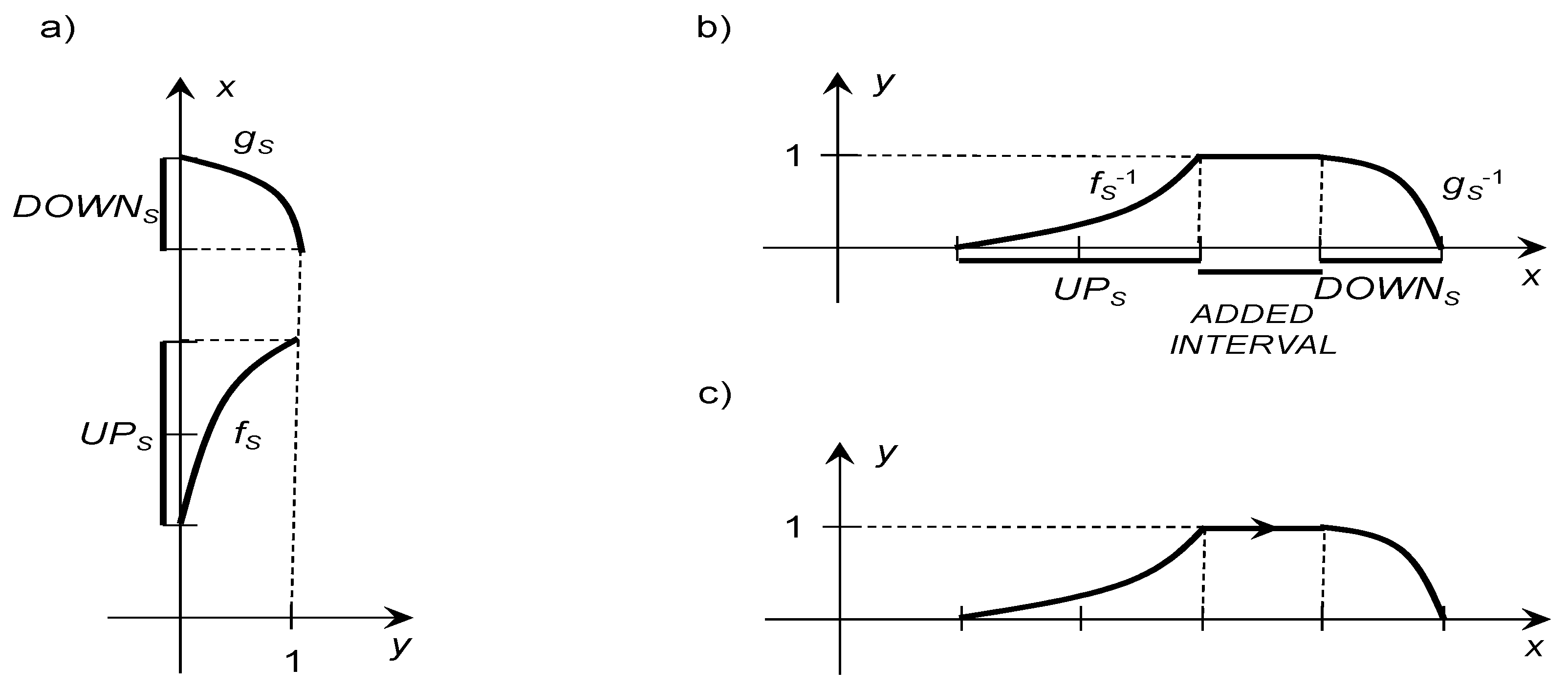
For any sequence$\left(a,b,c,d\right)\subset ℝ$, the KN$\overleftrightarrow{S}\left(a,b,c,d,\langle f_s\rangle {}^{⊲},\langle g_s\rangle {}^{⊲}\right)$is defined as an ordered pair$\left(f_S,g_S\right)$of monotonic continuous surjections$f_S:\left[0,1\right]\to U{P}_S=\left[a,b\right]$ and$g_S:\left[0,1\right]\to {\mathit{DOWN}}_S=\left[c,d\right]$fulfilling the condition:

$$f_s\left(0\right)=aand{f}_s\left(1\right)=band{g}_s\left(1\right)=cand{g}_s\left(0\right)=d.$$

(4)

For any KN $\overleftrightarrow{S}\left(a,b,c,d,\langle f_s\rangle {}^{⊲},\langle g_s\rangle {}^{⊲}\right)$, the function $f_S\in U{P}_s^{\left[0,1\right]}$ is called the up-function. Then, the function $g_S\in DOW{N}_s^{\left[0,1\right]}$ is called the down-function. Moreover, for KN $\overleftrightarrow{S}\left(a,b,c,d,\langle f_s\rangle {}^{⊲},\langle g_s\rangle {}^{⊲}\right)$, the number $a\in ℝ$ is called the starting point and the number $d\in ℝ$ is called the ending point. The space of all KNs is denoted by the symbol $\check{\mathbb{K}}$. Any sequence $\left(a,b,c,d\right)\subset ℝ$ satisfies exactly one of the following conditions:

$$b<c\parallel (b=canda<d),$$

(5)

$$b>c\parallel (b=canda>d),$$

(6)

$$b=canda=d.$$

(7)

If the condition (5) is fulfilled, then the KN $\overleftrightarrow{S}\left(a,b,c,d,\langle f_s\rangle {}^{⊲},\langle g_s\rangle {}^{⊲}\right)$ has a positive orientation. For this case, an example of graphs of KN is presented in Figure 1a. Any positively oriented K’N is interpreted as an imprecise number, which may increase. If the condition (6) is fulfilled, then KN $\overleftrightarrow{S}\left(a,b,c,d,\langle f_s\rangle {}^{⊲},\langle g_s\rangle {}^{⊲}\right)$ is negatively oriented. Then, it is interpreted as an imprecise number, which may decrease. For the case (7), KN $\overleftrightarrow{S}\left(a,b,c,d,\langle f_s\rangle {}^{⊲},\langle g_s\rangle {}^{⊲}\right)$ represents the interval $\left[a,b\right]\subset ℝ$.

In (Piasecki 2018) it is shown that we have:

Theorem 2.

For any sequence$\left(a,b,c,d\right)\subset ℝ$, the KN$\overleftrightarrow{S}\left(a,b,c,d,\langle f_s\rangle {}^{⊲},\langle g_s\rangle {}^{⊲}\right)$is explicitly determined by its membership relation${\mu }_s\left(·|a,b,c,d,\langle f_s\rangle {}^{⊲},\langle g_s\rangle {}^{⊲}\right)\subset ℝ\times \left[0,1\right]$given by the identity:

$${\mu }_L\left(x|a,b,c,d,,\langle f_s\rangle {}^{⊲},\langle g_s\rangle {}^{⊲}\right)=\{\begin{array}{cc}0,& x\notin \left[a,d\right]\equiv \left[d,a\right],\\ \langle f_s\rangle {}^{⊲}\left(x\right),& x\in \left[a,b\right]\equiv \left[b,a\right],\\ 1,& x\in \left[b,c\right]\equiv \left[c,b\right],\\ \langle g_s\rangle {}^{⊲}\left(x\right),& x\in \left[c,d\right]\equiv \left[d,c\right].\end{array}$$

(8)

The graph of membership function of KN $\overleftrightarrow{S}\left(a,b,c,d,f_S^{⊲},g_S^{⊲}\right)$ is presented in Figure 1b. A membership relation of any KN may be represented by the graph which has an extra arrow from the starting point to the ending one. This arrow denotes the KN orientation, which shows supplementary information about possible changes of the approximated number. The graph of KN membership function with positive orientation is shown in Figure 1c. Next, examples of such graphs are presented in Figure 2.

If the sequence $\left(a,b,c,d\right)\subset ℝ$ is not monotonic, then the membership relation ${\mu }_s\left(x|a,b,c,d,\langle f_s\rangle {}^{⊲},\langle g_s\rangle {}^{⊲}\right)\subset ℝ\times \left[0,1\right]$ is not a function. Then, this membership relation cannot be considered as a membership function of any fuzzy set. Therefore, for any non-monotonic sequence $\left(a,b,c,d\right)\subset ℝ$, the KN $\mathcal{S}\left(a,b,c,d,f_S^{⊲},g_S^{⊲}\right)$ is called an improper one (Kosiński 2006). An example of a membership relation of a negatively oriented improper KN is presented in Figure 3. The remaining KNs are called proper ones. Some examples of proper KNs were presented in Figure 2.

Kosiński et al. (2002, 2003) determined arithmetic operators for KNs as an extension of results obtained for FNs in (Goetschel and Voxman 1986). In our paper, we do not apply this arithmetic. Therefore, a description of arithmetic operations on FNs is omitted here.

Because in this paper we restrict our main considerations to the case of trapezoidal numbers, we will take into account the following definition:

Definition 2.

For any sequence$\left(a,b,c,d\right)\subset ℝ$, the trapezoidal KN (TrKN)$\overleftrightarrow{Tr}\left(a,b,c,d\right)$is defined as KN determined by its membership relation${\mu }_{Tr}\left(·|a,b,c,d\right)\subset ℝ\times \left[0,1\right]$given by the identity:

$${\mu }_T\left(x\right)={\mu }_{Tr}\left(x|a,b,c,d\right)=\{\begin{array}{cc}0,& x\notin \left[a,d\right]\equiv \left[d,a\right],\\ \frac{x-a}{b-a},& x\in \left[a,b\right]\equiv \left[b,a\right]\\ 1,& x\in \left[b,c\right]\equiv \left[c,b\right]\\ \frac{x-d}{c-d},& x\in \left[c,d\right]\equiv \left[d,c\right].\end{array}$$

(9)

The symbol ${\check{\mathbb{K}}}_{Tr}$ denotes the space of all TrKNs. Some examples of membership relations of TrKN are presented in Figure 2 and Figure 3.

Kosiński et al. (2002, 2003) determine arithmetic operators for TrKNs in the following way:

• The “dot multiplication” $⊡$ defined for any pair $\left(\beta ,\overleftrightarrow{Tr}\left(a,b,c,d\right)\right)\in ℝ\times {\check{\mathbb{K}}}_{Tr}$ by the identity:

  $$\beta ⊡\overleftrightarrow{Tr}\left(a,b,c,d\right)=\overleftrightarrow{Tr}\left(\beta ·a,\beta ·b,\beta ·c,\beta ·d\right),$$

  (10)
• The “Kosiński’s addition” ${⊞}_K$ defined for any pair $\left(\overleftrightarrow{Tr}\left(a,b,c,d\right),\overleftrightarrow{Tr}\left(e,f,g,h\right)\right)\in {\left({\check{\mathbb{K}}}_{Tr}\right)}^2$ by the identity:

  $$\overleftrightarrow{Tr}\left(a,b,c,d\right){⊞}_K\overleftrightarrow{Tr}\left(e,f,g,h\right)=\overleftrightarrow{Tr}\left(a+e,b+f,c+g,d+h\right).$$

  (11)

The determining “dot multiplication” is coherent with the Zadeh’s extension principle. On the other hand, “Kosiński’s addition” is not coherent with the Zadeh’s extension principle. In (Kosiński 2006) it is shown that there exist such pairs of proper TrKNs that their Kosiński’s sum is an improper one. This is the main reason why Kosiński’s theory of OFNs was revised in (Piasecki 2018).

2.2. Oriented Fuzzy Numbers

Only in the case of any monotonic sequence $\left(a,b,c,d\right)\subset ℝ$ may the membership relation ${\mu }_s\left(·|a,b,c,d,\langle f_s\rangle {}^{⊲},\langle g_s\rangle {}^{⊲}\right)\subset ℝ\times \left[0,1\right]$ be interpreted as a membership function ${\mu }_s\left(·|a,b,c,d,\langle f_s\rangle {}^{⊲},\langle g_s\rangle {}^{⊲}\right)\in {\left[0,1\right]}^{ℝ}$. Thus, we distinguish the following kind of proper OFN.

Definition 3.

(Piasecki 2018) For any monotonic sequence $\left(a,b,c,d\right)\subset ℝ$, the oriented fuzzy number (OFN) $\overleftrightarrow{L}\left(a,b,c,d,S_L,E_L\right)=\overleftrightarrow{ℒ}$ is the pair of orientation $\overrightarrow{a,d}=\left(a,d\right)$ and fuzzy set $ℒ\in ℱ(ℝ)$ described by membership function ${\mu }_L\left(\cdot |a,b,c,d,S_L,E_L\right)\in {\left[0,1\right]}^{ℝ}$ given by the identity:

$${\mu }_L\left(x|a,b,c,d,S_L,E_L\right)=\{\begin{array}{cc}0,& x\notin \left[a,d\right]\equiv \left[d,a\right],\\ S_L\left(x\right),& x\in \left[a,b\right]\equiv \left[b,a\right],\\ 1,& x\in \left[b,c\right]\equiv \left[c,b\right],\\ E_L\left(x\right),& x\in \left[c,d\right]\equiv \left[d,c\right].\end{array}$$

(12)

where the starting function $S_L\in {\left[0,1\right]}^{\left[a,b\right]}$ and the ending function $E_L\in {\left[0,1\right]}^{\left[c,d\right]}$ are upper semi-continuous monotonic ones meeting the conditions (3) and

$$S_L\left(b\right)=E_L\left(c\right)=1.$$

(13)

The symbol $\mathbb{K}$ denotes the space of all OFNs. Any OFN is a proper KN and any proper KN is OFN. Therefore, we have $\mathbb{K}\subset \check{\mathbb{K}}$. The positive and negative orientations of OFN are determined in the same way as for the case of KN. The interpretation of a OFN orientation is identical to the interpretation of a KN orientation. For the family of all positively oriented OFNs and the family of all negatively oriented OFN, we respectively denote by the symbols ${\mathbb{K}}^{+}$ and ${\mathbb{K}}^{-}$. For any OFN $\overleftrightarrow{L}\left(a,b,c,d,S_L,E_L\right)$, the condition (7) implies that:

$$a=b=c=d.$$

(14)

Then, the OFN $\overleftrightarrow{L}\left(a,a,a,a,S_L,E_L\right)=⟦a⟧$ describes the real number $a\in ℝ$ which is not oriented. Summing up, we see that:

$$\mathbb{K}={\mathbb{K}}^{+}{{\displaystyle \cup }}^{}ℝ{{\displaystyle \cup }}^{}{\mathbb{K}}^{-}.$$

(15)

We restrict our main considerations to the case of trapezoidal OFN, defined as follows:

Definition 4.

For any monotonic sequence$\left(a,b,c,d\right)\subset ℝ$, the trapezoidal OFN (TrOFN)$\overleftrightarrow{Tr}\left(a,b,c,d\right)$is defined as OFN determined with use its membership function${\mu }_{Tr}\left(·|a,b,c,d\right)\in {\left[0,1\right]}^{ℝ}$given by identity (9).

The symbol ${\mathbb{K}}_{Tr}$ denotes the space of all TrOFNs. In our considerations, we will only use the arithmetic operators determined for TrOFN. Then, the“Kosiński addition” ${⊞}_K$ is replaced by “addition” $⊞$ defined for any pair $\left(\overleftrightarrow{Tr}\left(a,b,c,d\right),\overleftrightarrow{Tr}\left(p-a,q-b,r-c,s-d\right)\right)\in {\left({\mathbb{K}}_{Tr}\right)}^2$ by the identity:

$$\begin{gathered} \overleftrightarrow{Tr}\left(a,b,c,d\right)⊞\overleftrightarrow{Tr}\left(p-a,q-b,r-c,s-d\right) \\ =\{\begin{array}{c}\overleftrightarrow{Tr}\left(\min \left\{p,q\right\},q,r,\max \left\{r,s\right\}\right),\left(q<r\right)\vee \left(q=r\wedge p\le s\right),\\ \overleftrightarrow{Tr}\left(\max \left\{p,q\right\},q,r,\min \left\{r,s\right\}\right),\left(q>r\right)\vee \left(q=r\wedge p>s\right).\end{array} \end{gathered}$$

(16)

The space ${\mathbb{K}}_{Tr}$ is closed under the addition $⊞$ (Piasecki 2018). Moreover, sums obtained by using the addition $⊞$ are the best approximation of sums obtained by means of the Kosiński’s addition ${⊞}_K$ (Piasecki 2018). The restrictions imposed in Definition 4 allow that TrOFNs may be analyzed with use of the fuzzy set theory. On the other hand, these methods of analysis are not applicable for TrKNs. Therefore, if we intend to apply trapezoidal OFNs for any additive model, then we should restrict our considerations to the use of the additive semigroup $\langle {\mathbb{K}}_{Tr},⊞\rangle$. This principle is shortly called the postulate restricting applications to the use of TrOFNs. It is very important restriction because we have many additive models of real-world problems. For example, financial portfolio analysis is an additive model.

Furthermore, the addition $⊞$ is not commutative. It implies that any multiple sum determined by $⊞$ may be dependent on its summands’ ordering (Piasecki 2018). For this reason, the assumed order of performing multiple additions may require additional justifications.

For any OFN, the “dot multiplication” operator is determined by the identity (10). As we know, the “dot multiplication” is coherent to the Zadeh’s extension principle. Therefore, using this principle, we can extend the “dot multiplication” operator to any unary operator linked to monotonic function $G:ℝ\supset \mathbb{A}\to ℝ$. This extension is determined in the following way:

If TrOFN $\overleftrightarrow{Tr}\left(a,b,c,d\right)$ is represented by its membership function ${\mu }_{Tr}\left(·|a,b,c,d\right)\in {\left[0,1\right]}^{ℝ}$, then the membership function ${\mu }_G\in {\left[0,1\right]}^{ℝ}$ of OFN $\overleftrightarrow{\mathcal{G}}=G\left(\overleftrightarrow{Tr}\left(a,b,c,d\right)\right)$ is given by the identity:

$${\mu }_G\left(x\right)={\mu }_{Tr}\left(G^{-1}\left(x\right)|G\left(a\right),G\left(b\right),G\left(c\right),G\left(d\right)\right).$$

(17)

While discussing the results obtained, we will also refer to the disorientation map $\overline{\overline{\mathsf{\Psi }}}:\mathbb{K}\to \mathbb{F}$ determined in (Piasecki 2019) as follows:

$$\overline{\overline{\mathsf{\Psi }}}\left(\overleftrightarrow{ℒ}\left(a,b,c,d,S_L,E_L\right)\right)=\{\begin{array}{c}L\left(a,b,c,d,S_L,E_L\right)\overleftrightarrow{ℒ}\left(a,b,c,d,S_L,E_L\right)\in {\mathbb{K}}^{+}{{\displaystyle \cup }}^{}R,\\ L\left(d,c,b,a,E_L,S_L\right)\overleftrightarrow{ℒ}\left(a,b,c,d,S_L,E_L\right)\in {\mathbb{K}}^{-}.\end{array}$$

(18)

3. Japanese Candlesticks

We understand the term “security” as an authorization to receive a future financial revenue, payable to a certain maturity. Japanese Candlestick (JC) is a kind of financial chart used to describe the volatility of a fixed security quotation. The JC charting techniques are perfectly described by Nison (1991). The basic elements of JC charting techniques are the descriptions of a single JC.

Let fixed security be given as $\mathcal{Y}$. For the assumed time period $\left[0,T\right]$, the volatility of the security $\mathcal{Y}$ quotations are described by the function $Q:\left[0,T\right]\to {ℝ}^{+}$. Then, JC represents four important pieces of information about $\mathcal{Y}$ quotations:

• The open price:

  $$P_o=Q\left(0\right),$$

  (19)
• The close price:

  $$P_c=Q\left(T\right),$$

  (20)
• The high price:

  $$P_h=\max \left\{Q\left(t\right):t\in \left[0,T\right]\right\},$$

  (21)
• The low price:

  $$P_l=\min \left\{Q\left(t\right):t\in \left[0,T\right]\right\}.$$

  (22)

The high price and the low price together are called extreme prices. In brokerage house reports, each JC is usually described by the data set $\left\{P_o,P_c,P_l,P_h\right\}$ of reported prices. In general, JCs are optional composed of:

• The body determined as a rectangle between the open price and the closed price.
• The upper wick determined as the line between the body and the high price.
• The lower wick determined as the line between the body and the low price.

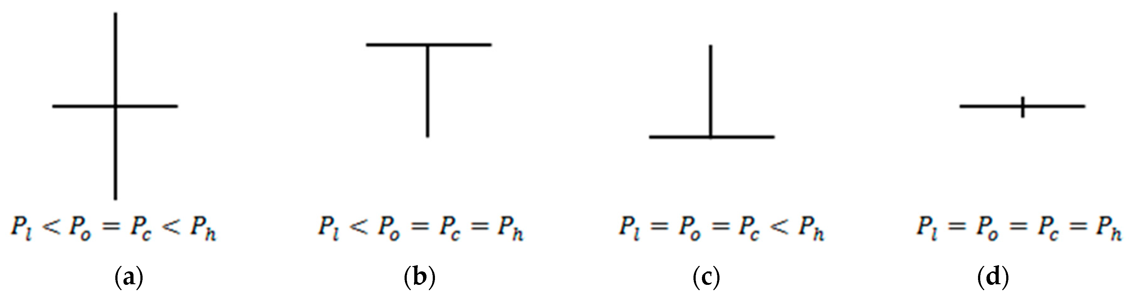
The body illustrates the opening and closing trades. We can note the following cases here:

$$P_o<P_c,$$

(23)

$$P_o>P_c,$$

(24)

$$P_o=P_c,$$

(25)

If the condition (23) is met, then the candle body is white. Then, the JC is called White Candle or White Spinning. Any Black Candle may be considered as a bullish signal, i.e., a forecast of an increase in quotations. If the condition (24) is satisfied, then the candle body is black. Then, the JC is called Black Candle or Black Spinning. Any Black Candle may be considered as a bearish signal, i.e., a forecast of a decline in quotations. The general case of a White Candle and a Black Candle are presented in the Figure 4.

Any JC need not have either a body or a wick. If a JC fulfills the condition (25) then it does not have a body. Such a JC is called a Doji. We distinguish the following main kinds of Doji:

• Doji Star is a JC fulfilling the condition:

  $$P_l<P_o=P_c<P_h,$$

  (26)
• Dragonfly Doji is a JC fulfilling the condition:

  $$P_l<P_o=P_c=P_h,$$

  (27)
• Gravestone Doji is a JC fulfilling the condition:

  $$P_l=P_o=P_c<P_h,$$

  (28)
• Four Price Doji is a JC fulfilling the condition:

  $$P_l=P_o=P_c=P_h,$$

  (29)

These kinds of Doji are presented in Figure 5.

Example 1.

During the session on the Warsaw Stock Exchange (WSE) on July 23, 2019, we observed quotations of the following companies: Assecopol (ACP), CYFRPLSAT (CPS), ENERGA (ENG), JSW (JSW), KGHM (KGH), LOTOS (LTS), ORANGEPL (OPL), PGE(PGE), PKOBP (PKO). For each observed company, the results of our observations are recorded in

Table 1. Selected quotations on the Warsaw Stock Exchange (WSE) on 23 July, 2019. Source: (Bankier.pl n.d.) and own elaboration.

Company	$\mathbf{Open}\mathbf{Price}{\mathit{P}}_{\mathit{o}}$	$\mathbf{Close}\mathbf{Price}{\mathit{P}}_{\mathit{c}}$	$\mathbf{Low}\mathbf{Price}{\mathit{P}}_{\mathit{l}}$	$\mathbf{High}\mathbf{Price}{\mathit{P}}_{\mathit{h}}$	Kind of JC
ACP	56.00	56.55	56.00	57.15	White Candle
CPS	30.14	30.00	29.74	30.24	Black Candle
ENG	7.60	7.60	7.58 *	7.71 **	Doji Star
JSW	42.60	41.92	41.80	42.68	Black Candle
KGH	97.50	96.62	95.94	97.96	Black Candle
LTS	88.70	87.48	86.82	88.70	Black Candle
OPL	6.18	6.38	6.17	6.47	White Candle
PGE	9.48	9.32	9.25	9.57	Black Candle
PKO	42.60	42.60	42.49 **	42.79 *	Doji Star

* Earlier extreme price $P_{xe}$ ** later extreme price $P_{xl}$.

as reported price sets.

Each reported price set may be graphically presented by the JC mentioned in the last column of Table 1. Furthermore, we see that the quotations of ACP are assigned with a White Candle without a lover wick. In addition, all extreme prices are marked here with stars. The notions of earlier and later extreme prices are explained in Section 5.

4. Modeling of Japanese Candlesticks by Kosiński’s Numbers

Let us take into account two facts:

• Any OFN may be interpreted as an imprecise approximation of a real number, which may change in direction determined by orientation.
• Each JC may be used as such an approximation of market price that it is additionally equipped with information about this price trend.

For this reason, any JC may be represented by means of OFN. In this section, we focus our attention on the use of KN for modeling candles. In the literature we find two such models.

4.1. The Marszałek’s Approach

Let fixed security be given as $\mathcal{Y}$ quoted in the assumed time period $\left[0,T\right]$, Marszałek and Burczyński (2013a, 2013b, 2014) consider the observed quotation trend $Q:\left[0,T\right]\to {ℝ}^{+}$ as a realization of random variable. Considered security, $\mathcal{Y}$, can be represented by the following parameters: the open price $P_o$, the close price $P_c$, the high price $P_h$, and the low price $P_l$.

At the beginning, the authors select two real numbers, $S_1,S_2\in ℝ$, fulfilling the condition:

$$P_l<S_1\le S_2<P_h.$$

(30)

Then, they calculate conditional probabilities:

$$f_q\left(x\right)=P\left(Q\left(t\right)>x|Q\left(t\right)>S_2\right),$$

(31)

$$g_q\left(x\right)=P\left(Q\left(t\right)<x|Q\left(t\right)<S_1\right).$$

(32)

The above probabilities determine the functions $f_q:\left[S_2,P_h\right]\to \left[0,1\right]$ and $g_q:\left[P_l,S_1\right]\to \left[0,1\right]$. Different methods of determining numbers $S_1,S_2$ and estimating the probabilities (31) and (32) are discussed in (Marszałek and Burczyński 2013a, 2013b, 2014). However, in all the examples given there we observe that:

$$P_o<S_1\le S_2<P_c.$$

(33)

This restriction results from the requirements of probability estimation methods. Finally, authors save the observed quotation trend $Q:\left[0,T\right]\to {ℝ}^{+}$ as KN $\overleftrightarrow{\mathcal{Q}}\in \check{\mathbb{K}},$ determined in the following way:

$$\overleftrightarrow{\mathcal{Q}}=\overleftrightarrow{S}\left(a,b,c,d,\langle f_s\rangle {}^{⊲},\langle g_s\rangle {}^{⊲}\right)=\{\begin{array}{c}\overleftrightarrow{S}\left(P_l,S_1,S_2,P_h,\langle g_q\rangle {}^{⊲},\langle f_q\rangle {}^{⊲}\right)P_o<P_c\\ \overleftrightarrow{S}\left(P_h,S_2,S_1,P_l,\langle f_q\rangle {}^{⊲},\langle g_q\rangle {}^{⊲}\right)P_o>P_c\end{array}.$$

(34)

It is easy to see that the essence of the above KN is similar to the JC essence. For this reason, we agree with Marszałek and Burczyński that the above KN $\overleftrightarrow{\mathcal{Q}}$ may be called oriented fuzzy candlestick (OFC). In our opinion, OFCs are an excellent short record of quotation volatility. In (Marszałek and Burczyński 2013a, 2013b, 2014), it is shown that OFC is very useful for financial decision making. Unfortunately, OFC does not save information about the low price $P_l$ and high price $P_h$. Therefore, any OFC is not a quantitative model of JC.

4.2. The Kacprzak’s Approach

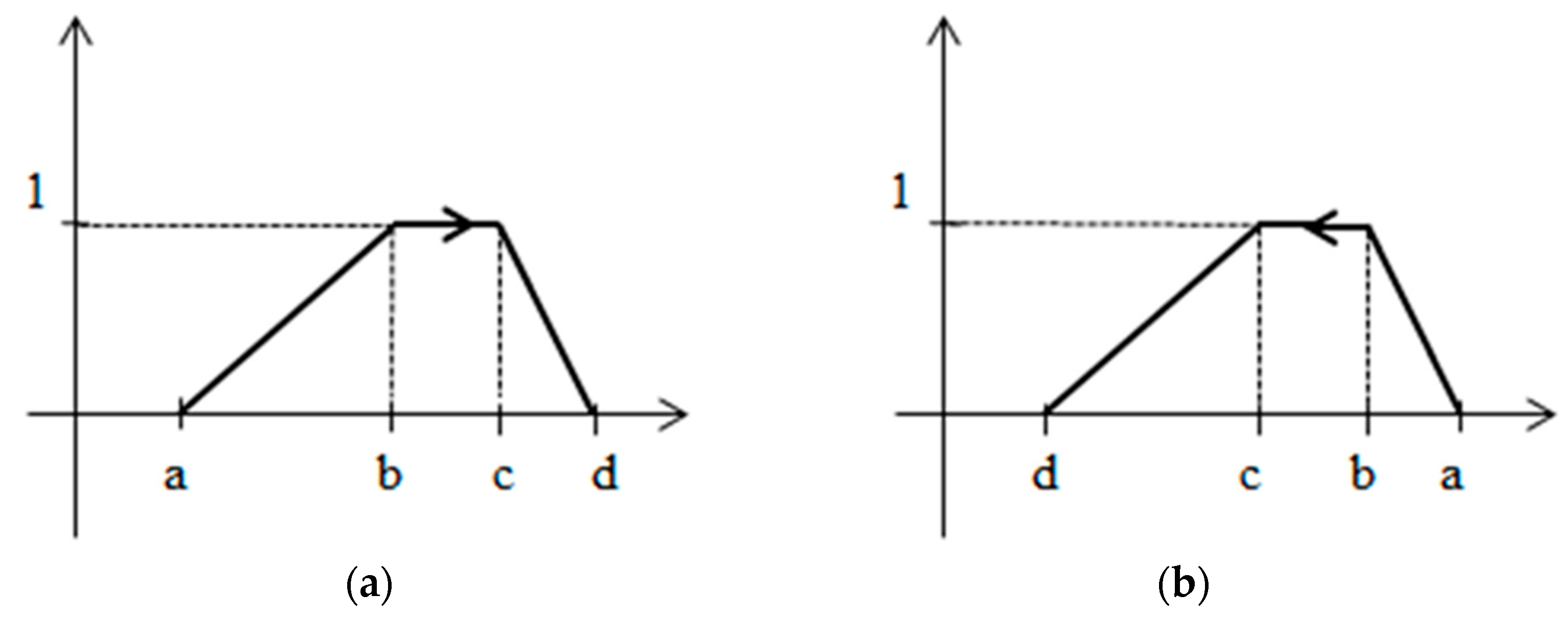
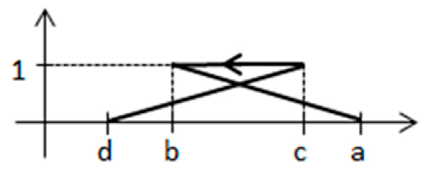
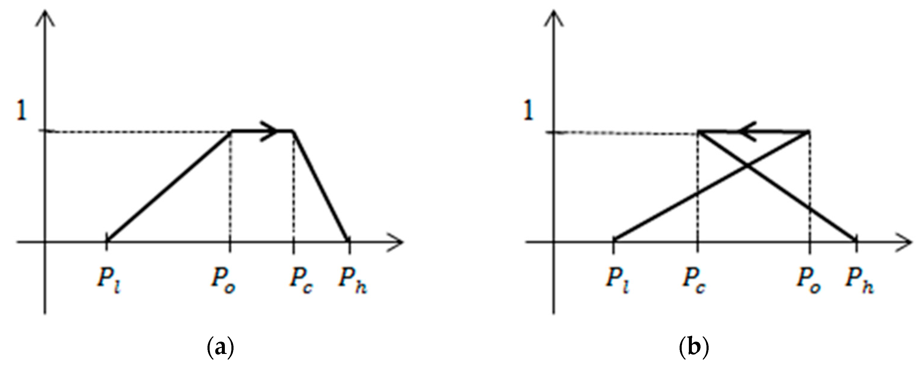
Kacprzak et al. (2013) propose ex cathedra the universal way of presenting JC as TrKN $\overleftrightarrow{Tr}\left(P_l,P_o,P_c,P_h\right)$. Then, any White Candle is represented by positively oriented TrKN, which is a proper one. The membership function of this White Candle is presented in Figure 6a. In line with the Kacprzak’s approach, any Black Candle is described by negatively oriented TrKN, which is an improper one. In Figure 6b, we can see the graph of a membership relation describing a Black Candle. Any Doji is represented by proper TrKN.

Example 2.

We describe each Japanese candle observed in Example 1 by TrKN determined by means of the Kacprzak’ method. Obtained representations are presented in

Table 2. Representation of Japanese candles observed in Example 1 in the WSE on 23 July, 2019. Black: proper KN; Red: improper KN; Green: positively oriented FN; Blue: negatively oriented FN.

Company	Kacprzak’s Method of Representation by TrKN	Proposed Method of Representation by TrOFN
ACP	$\overleftrightarrow{Tr}\left(56.00,56.00,56.55,57.15\right)$	${\overleftrightarrow{\mathcal{J}\mathcal{C}}}_{ACP}=\overleftrightarrow{Tr}\left(56.00,56.00,56.55,57.15\right)$
CPS	$\overleftrightarrow{Tr}\left(29.74,30.14,30.00,30.24\right)$	${\overleftrightarrow{\mathcal{J}\mathcal{C}}}_{CPS}=\overleftrightarrow{Tr}\left(30.24,30.14,30.00,29.74\right)$
ENG	$\overleftrightarrow{Tr}\left(7.58,7.60,7.60,7.71\right)$	${\overleftrightarrow{\mathcal{J}\mathcal{C}}}_{ENG}=\overleftrightarrow{Tr}\left(7.58,7.60,7.60,7.71\right)$
JSW	$\overleftrightarrow{Tr}\left(41.80,42.60,41.92,42.68\right)$	${\overleftrightarrow{\mathcal{J}\mathcal{C}}}_{JSW}=\overleftrightarrow{Tr}\left(42.68,42.60,41.92,41.80\right)$
KGH	$\overleftrightarrow{Tr}\left(95.94,97.50,96.62,97.96\right)$	${\overleftrightarrow{\mathcal{J}\mathcal{C}}}_{KGH}=\overleftrightarrow{Tr}\left(97.96,97.50,96.62,95.94\right)$
LTS	$\overleftrightarrow{Tr}\left(86.82,88.70,87.48,88.70\right)$	${\overleftrightarrow{\mathcal{J}\mathcal{C}}}_{LTS}=\overleftrightarrow{Tr}\left(88.70,88.70,87.48,86.82\right)$
OPL	$\overleftrightarrow{Tr}\left(6.17,6.18,6.38,6.47\right)$	${\overleftrightarrow{\mathcal{J}\mathcal{C}}}_{OPL}=\overleftrightarrow{Tr}\left(6.17,6.18,6.38,6.47\right)$
PGE	$\overleftrightarrow{Tr}\left(9.25,9.48,9.32,9.57\right)$	${\overleftrightarrow{\mathcal{J}\mathcal{C}}}_{PGE}=\overleftrightarrow{Tr}\left(9.57,9.48,9.32,9.25\right)$
PKO	$\overleftrightarrow{Tr}\left(42.49,42.60,42.60,42.79\right)$	${\overleftrightarrow{\mathcal{J}\mathcal{C}}}_{PKO}=\overleftrightarrow{Tr}\left(42.79,42.60,42.60,42.42\right)$

. All improper TrKNs are indicated in red.

To our best knowledge, for the moment, the described Kacprzak’s representation of JCs have not found an application in finance theory or practice. We suppose that it results from the fact that Kacprzak’s approach to JCs’ modeling is not coherent with the postulate restricting applications to the use of TrOFNs. Thus, in the next section, we will propose a universal model of representing JCs by TrOFN.

5. Representation of Japanese Candlesticks by Trapezoidal Oriented Fuzzy Numbers (TrOFN)

In above section, we conclude that any JC should be represented by TrOFN. That is why we are reconsidering the fixed JC, $\widetilde{\mathcal{J}\mathcal{C}}$. Let $\widetilde{\mathcal{J}\mathcal{C}}$ be reported by the data set $\left\{P_o,P_c,P_l,P_h\right\}$ of reported prices. Then, $\widetilde{\mathcal{J}\mathcal{C}}$ may be represented by a TrOFN $\overleftrightarrow{Tr}\left(\alpha ,\beta ,\gamma ,\delta \right),$ where a sequence $\left(\alpha ,\beta ,\gamma ,\delta \right)$ is a monotonic permutation of all reported prices. Moreover, it is obvious that the TrOFN $\overleftrightarrow{Tr}\left(\alpha ,\beta ,\gamma ,\delta \right)$ should be oriented from open price $P_o$ to close price $P_c$. It means that in a general case, any sequence $\left(\alpha ,\beta ,\gamma ,\delta \right)$ contains the subsequence $\left(P_o,P_c\right)$. From dependences (19)–(22), we get:

$$P_l\le \min \left\{P_o,P_c\right\}\le \max \left\{P_o,P_c\right\}\le P_h.$$

(35)

We see that in a general case, the starting point and ending point are extreme prices. Therefore, any $\widetilde{\mathcal{J}\mathcal{C}}$ may be be represented only by a TrOFN $\overleftrightarrow{Tr}\left(\alpha ,P_o,P_c,\delta \right)$ where the sequence $\left(\alpha ,\delta \right)$ is such a permutation of extreme prices that the sequence $\left(\alpha ,P_o,P_c,\delta \right)$ is monotonic. Looking for a universal method for determining the permutation $\left(\alpha ,\delta \right)$, in the first step, we will change the identification of extreme prices.

The orientation from open price, $P_o$, to close price, $P_c,$ may be determined unambiguously only for the case when $\widetilde{\mathcal{J}\mathcal{C}}$ has a body. It is equivalent to the condition:

$$P_o\ne P_c.$$

(36)

If the extreme price, $P_b\in \left\{P_l,Ph\right\},$ is closer to the open price, $P_o,$ than to the close price, $P_c,$ then the price, $P_b,$ is called the back price. In other words, the extreme price, $P_b\in \left\{P_l,Ph\right\},$ is called the back price if it fulfills the condition:

$$\left|P_b-P_o\right|\le \left|P_b-P_c\right|.$$

(37)

In this way, for the White Candle, the back price, $P_b,$ is equal to the low price, $P_l,$ and for the Black Candle, the back price, $P_b,$ is equal to the high price, $P_h$. If the extreme price, $P_f\in \left\{P_l,P_h\right\},$ is closer to the close price, $P_c,$ than to the open price, $P_o,$ then the price, $P_f,$ is called face price. In other words, the extreme price, $Pb\in \left\{P_l,P_h\right\},$ is called the face price if it fulfills the condition:

$$\left|P_f-P_c\right|\le \left|P_f-P_o\right|.$$

(38)

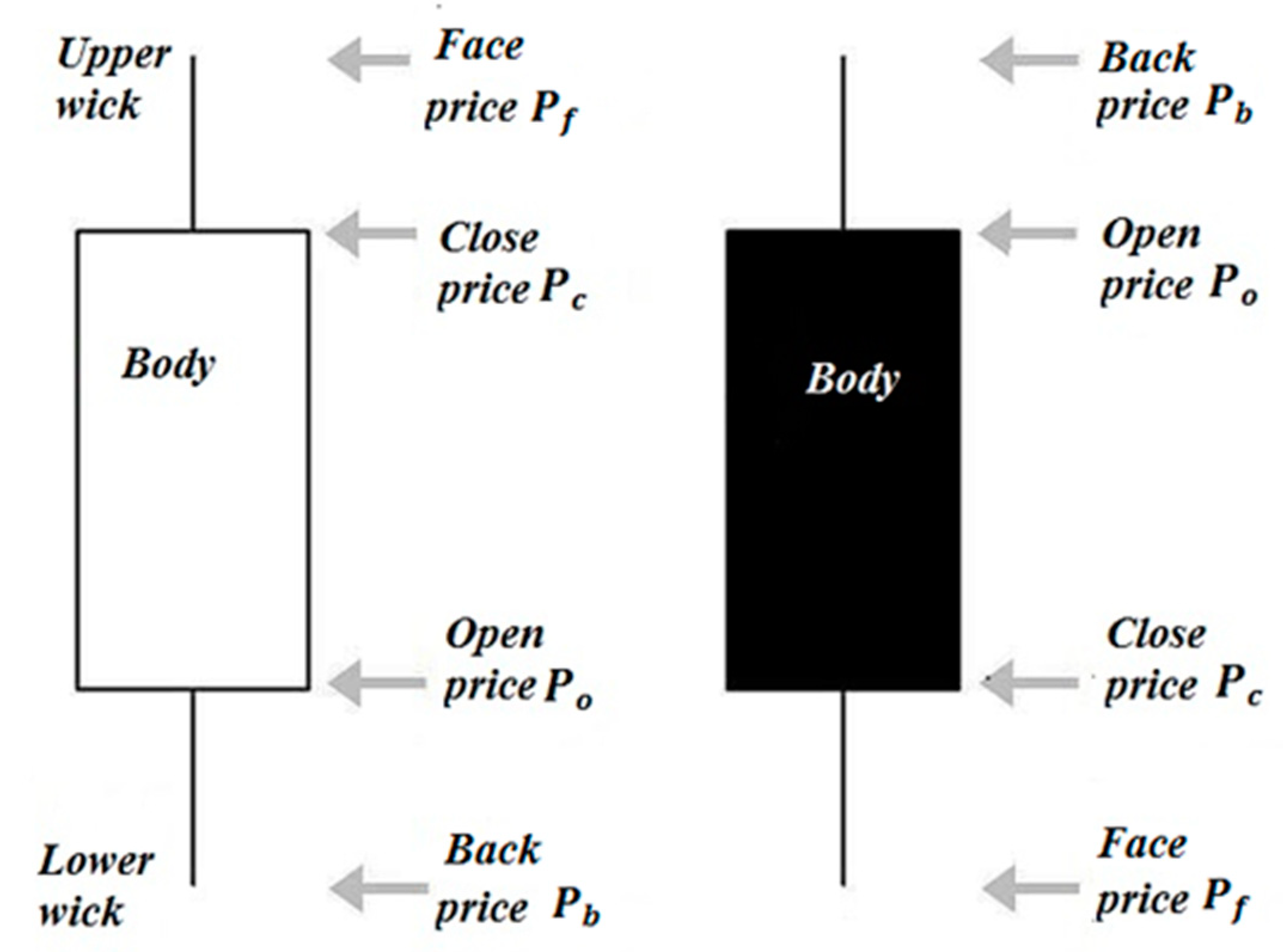
In this way, for the White Candle, the face price, $P_f,$ is equal to the high price, $P_h,$ and for the Black Candle, the face price, $P_f,$ is equal to the low price, $P_l$. Thanks to condition (36), the back price, $P_b,$ and the face price, $P_f,$ are determined explicitly. With this reinterpretation of extreme prices, we get a modernized model of JCs which have a body. The general cases of a White Candle and a Black candle are presented in Figure 7.

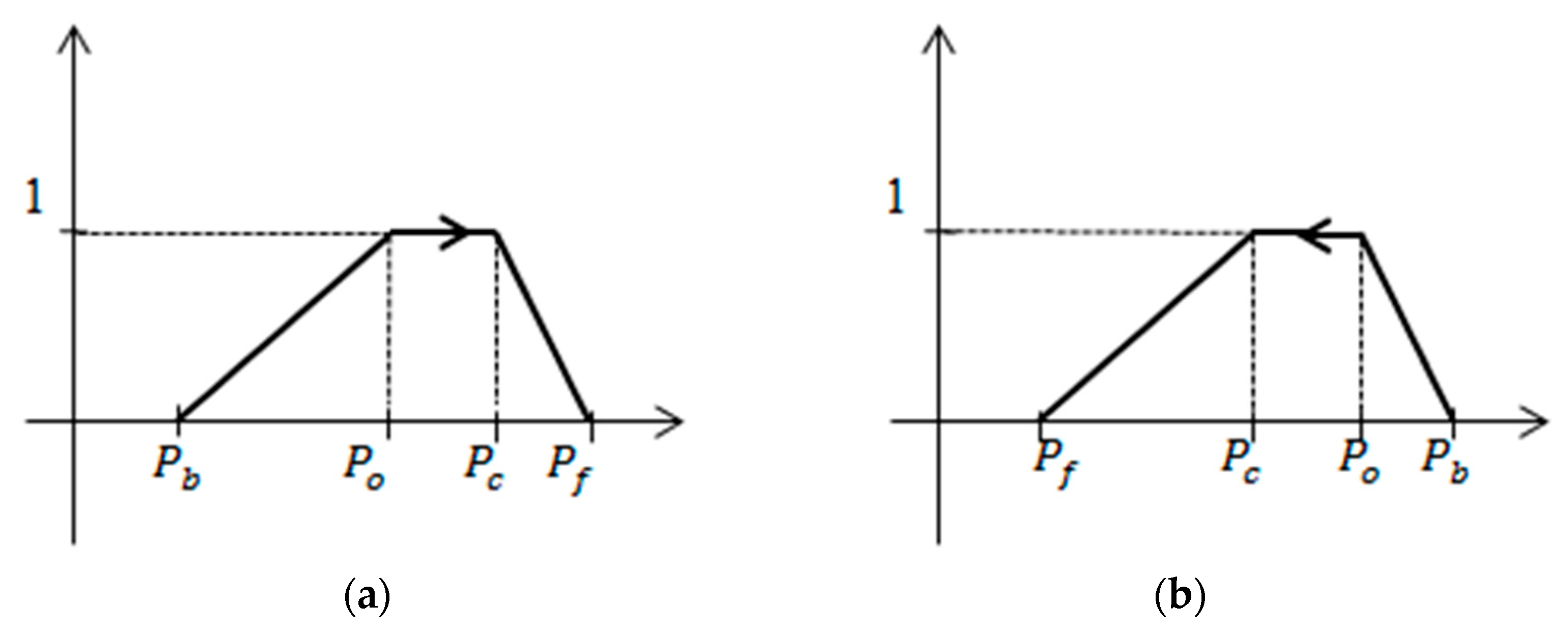
The sequence $\left(P_b,P_o,P_c,P_f\right)$ is the unique monotonic permutation of reported prices which contains the subsequence $\left(P_o,P_c\right)$. For this reason, we propose to describe the Japanese Candle, $\widetilde{\mathcal{J}\mathcal{C},}$ by the TrOFN, $\overleftrightarrow{Tr}\left(P_b,P_o,P_c,P_f\right)$. Then, any White Candle is represented by positively oriented TrOFN determined by the membership function presented in Figure 8a. In this representation, any Black Candle is described by negatively oriented TrOFN determined by the membership function presented in Figure 8b.

Now, we consider the case (25) when the considered $\widetilde{\mathcal{J}\mathcal{C}}$ is a Doji. Then, the inequality (35) implies that for any permutation $\left(\alpha ,\delta \right)$ of extreme prices, the sequence $\left(\alpha ,P_o,P_c,\delta \right)=\left(\alpha ,P_c,P_c,\delta \right)$ is monotonic. Then Doji $\widetilde{\mathcal{J}\mathcal{C}}$ may be represented by a TrOFN, $\overleftrightarrow{Tr}\left(\alpha ,P_c,P_c,\delta \right),$ where the subsequence $\left(\alpha ,\delta \right)$ is any permutation of extreme prices. On the other hand, in line with (5) and (6), the orientation of $\overleftrightarrow{Tr}\left(\alpha ,P_c,P_c,\delta \right)$ can only be determined as orientation from the starting point to the ending point. Furthermore, for any Doji, the back price, $P_b,$ and the face price, $P_f,$ are not explicitly determined. Thus, the orientation of TrOFN representing any Doji cannot be defined as the direction from a back price, $P_b,$ to a face price, $P_f$. For these reasons, we propose to present any Doji by TrOFN with orientation from the earlier extreme price, $P_{xe},$ to the later extreme price, $P_{xl}$.

The kinds of extreme prices mentioned above are determined in the following way. At the beginning, we assign each quotation $\widehat{Q}\in Q\left(\left[0,T\right]\right)$ the last moment $\tau \left(\widehat{Q}\right)$ of its observation defined by the identity:

$$\tau \left(\widehat{Q}\right)=\max \left\{t\in \left[0,T\right]:Q\left(t\right)=\widehat{Q}\right\}.$$

(39)

Let us consider now the case when:

$$P_l\ne P_h.$$

(40)

Then, we get:

$$\tau \left(P_l\right)\ne \tau \left(P_h\right)$$

(41)

Then, the earlier extreme price, $P_{xe},$ and later extreme price, $P_{xl},$ we define as follows:

$$P_{xe}=\{\begin{array}{c}{P}_l,\tau \left(P_l\right)<\tau \left(P_h\right),\\ P_h,\tau \left(P_l\right)>\tau \left(P_h\right),\end{array}$$

(42)

$$P_{xl}=\{\begin{array}{c}{P}_h,\tau \left(P_l\right)<\tau \left(P_h\right),\\ P_l,\tau \left(P_l\right)>\tau \left(P_h\right).\end{array}$$

(43)

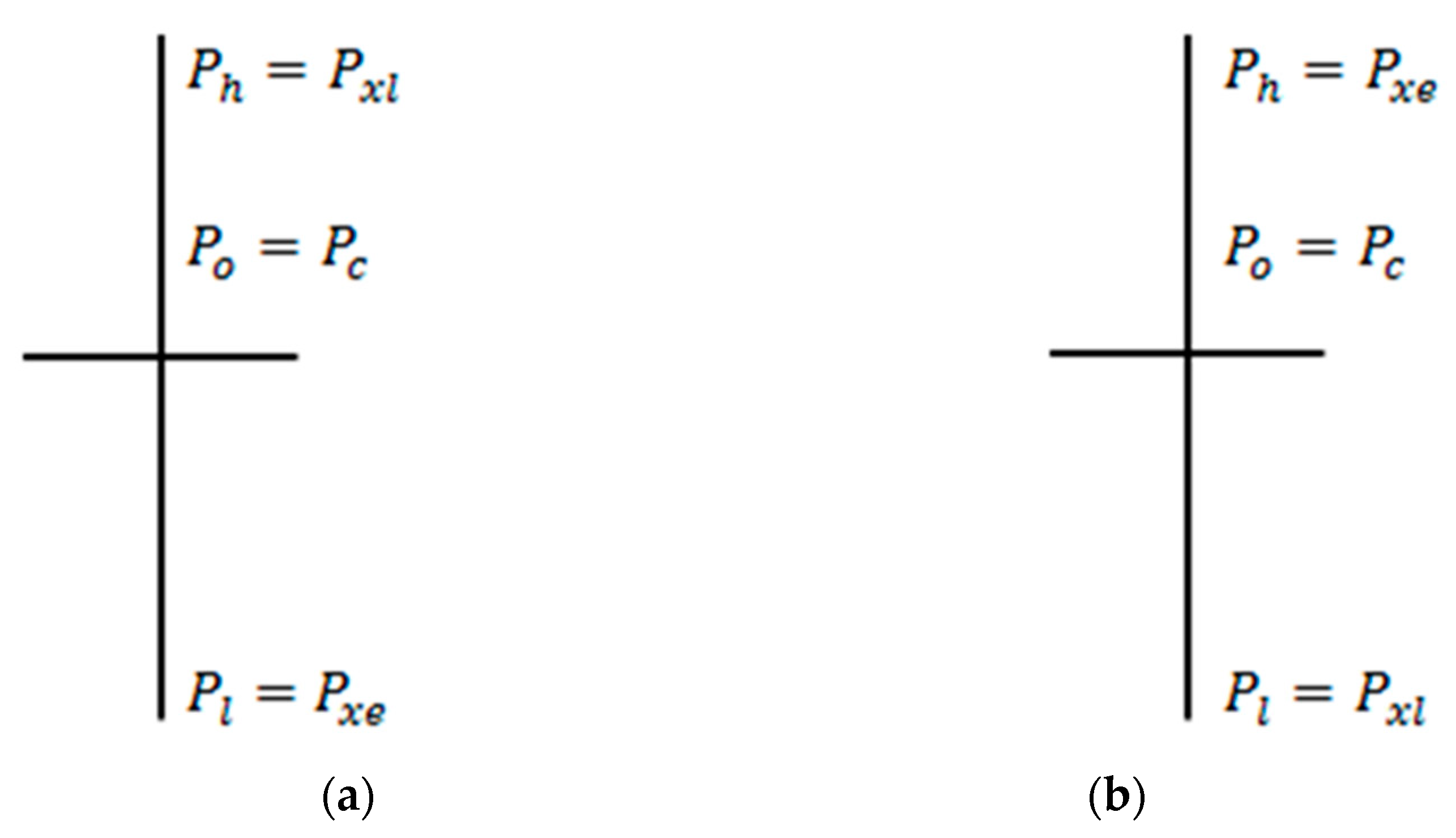
In this way, we interpret extreme prices as an earlier or later one. With this reinterpretation of extreme prices, we get a modernized model of Doji. The general cases Doji Stars are presented in Figure 9.

We propose to describe any Doji by TrOFN, $\overleftrightarrow{Tr}\left(P_{xe},P_c,P_c,P_{xl}\right)$. Then, the Doji Star presented in Figure 9a is described by the positively oriented TrOFN, $\overleftrightarrow{Tr}\left(P_l,P_c,P_c,P_h\right)$. The Doji Star presented in Figure 9b is described by the negatively oriented TrOFN, $\overleftrightarrow{Tr}\left(P_h,P_c,P_c,P_l\right)$. These representations of Doji are determined by their membership functions presented in Figure 10.

For any Dragonfly Doji we have:

$$\tau \left(P_h\right)=\tau \left(P_c\right)=T>\tau \left(P_l\right).$$

(44)

Thus, any Dragonfly Doji is represented by positively oriented TrOFN, $\overleftrightarrow{Tr}\left(P_l,P_c,P_c,P_c\right)$. This positive orientation is consistent with the common belief that any Dragonfly Doji could signal a potential bullish reversal of market quotations. The Dragonfly Doji modernized model is shown in Figure 11a.

For any Gravestone Doji we have:

$$\tau \left(P_l\right)=\tau \left(P_c\right)=T>\tau \left(P_h\right).$$

(45)

Therefore, any Gravestone Doji is represented by negatively oriented TrOFN, $\overleftrightarrow{Tr}\left(P_h,P_c,P_c,P_c\right)$. This negative orientation is consistent with the common belief that any Gravestone Doji could signal a potential bearish reversal of market quotations. The Gravestone Doji modernized model is shown in Figure 11b.

If the condition (40) is not satisfied, then we get:

$$P_l=P_o=P_c=P_h.$$

(46)

This case corresponds to the Four Price Doji, the modernized model of which is presented in Figure 11c. Any Four Price Doji is described by the TrOFN, $\overleftrightarrow{Tr}\left(P_c,P_c,P_c,P_c\right)=⟦P_c⟧,$ which is not oriented.

It is very easy to check that all types of Japanese candles omitted in the above specification are only special cases of the discussed candles.

Example 3.

We describe each Japanese candle observed in Example 1 by TrOFN determined by means of the method proposed by us. The quotations ACP and OPL are assigned with White Candles represented by TrOFNs in the form$\overleftrightarrow{Tr}\left(P_l,P_o,P_c,P_h\right)$. The quotations of CPS, JSW, KGH, LTS, and PGE OPL are assigned with Black Candles represented by TrOFNs in the form$\overleftrightarrow{Tr}\left(P_h,P_o,P_c,P_l\right)$. The quotations ENG and PKO are assigned with Doji Star. Therefore, we should determine an earlier extreme price$P_{xe}$and a later one$P_{xl}$for both companies.$Wearelookingforthesepricesbystudyingtick-data.$The results of this search are shown in Table 1. For ENG, we get$P_{xe}=P_l$and$P_{xl}=P_h$. Therefore, the quotations of ENG are assigned to Doji Star represented by TrOFN in the form$\overleftrightarrow{Tr}\left(P_l,P_c,P_c,P_h\right)$. For PKO, we obtain$P_{xe}=P_h$and$P_{xl}=P_l$. Therefore, the quotations of PKO are assigned to Doji Star represented by TrOFN in the form$\overleftrightarrow{Tr}\left(P_h,P_c,P_c,P_l\right)$. Obtained representations are presented in Table 2. All positively oriented TrOFNs are indicated in green. All negatively oriented TrOFNs are indicated in blue.

In summary, any JC can be represented by TrOFN:

$$\overleftrightarrow{JC}=\overleftrightarrow{Tr}\left(\alpha ,P_o,P_c,\delta \right)$$

(47)

where the sequence $\left(\alpha ,\delta \right)$ is such a permutation of extreme prices $\left\{P_l,P_h\right\}$ that it is determined by conditions (37) and (38) or by (42) and (43), or by (46).

Any security may be evaluated by a present value (PV) generally defined as a current equivalent value of payments at a fixed point in time (Piasecki 2012). It is commonly accepted that the PV of a future cash flow can be imprecise. The natural consequence of this approach is estimating PV with FNs. A detailed description of the evolution of this particular model can be found, for example in (Łyczkowska-Hanćkowiak and Piasecki 2018a). If an imprecisely estimated PV is additionally equipped with a forecast of its closest changes, then it is called oriented PV (OPV). It is obvious that any OPV should be represented by an OFN $\overleftrightarrow{PV}$.

Let us take into account the fixed security $\mathcal{Y}$. If the volatility of its quotations is characterized by JC (47) then we can determine its OPV as follows:

$$\overleftrightarrow{PV}\left(\mathcal{Y}\right)=\overleftrightarrow{JC}=\overleftrightarrow{Tr}\left(\alpha ,P_o,P_c,\delta \right).$$

(48)

Then, the OPV membership function ${\mu }_{Tr}\left(·|\alpha ,P_o,P_c,\delta \right)$ is determined by condition (9). Some applications of such an approximated OPV are given in Section 6 and Section 7.

6. Oriented Expected Return Determined by Japanese Candlestick

Let us assume that the time horizon $t>0$ of an investment is fixed. Then, the security $\mathcal{Y}$ considered here is determined by two values:

• Anticipated FV $V_t$ and
• Assessed PV $V_0$.

The basic characteristic of benefits from owning this security is a return rate $r_t$ given by the identity:

$$r_t=r\left(V_0,V_t\right)$$

(49)

In the general case, if $\left(V_0,V_t\right)\in {ℝ}^{+}\times {ℝ}^{+}$, then the function: $r:{ℝ}^{+}\times {ℝ}^{+}\to ℝ$ is a decreasing function of PV and an increasing function of FV. Moreover, in the special case, we have here:

• Simple return rate:

  $$r_t=\frac{V_t-V_0}{V_0}=\frac{V_t}{V_0}-1$$

  (50)
• Logarithmic return rate:

  $$r_t=\ln \frac{V_t}{V_0}.$$

  (51)

In this section, we restrict our considerations to the case of any simple return rate given by condition (50). Thanks to this, our considerations will be more clear. However, the results obtained can be easily generalized to the case of generalized return rate given by condition (49).

The security $\mathcal{Y}$ is an authorization to receive future financial revenue, payable to a certain maturity. The value of this revenue is interpreted as the anticipated FV of the security. According to the uncertainty theory introduced by Von Mises (1962) and Kaplan and Barish (1967), for anyone unknown to us, the future state of affairs is uncertain. The Mises–Kaplan uncertainty is a result of our lack of knowledge about the future state of affairs. Yet, in the researched case, we can point out this particular time in the future, in which the considered state of affairs will already be known to the observer. Behind (Kolmogorov 1933, 1956; Von Mises 1957; Von Lambalgen 1996; Caplan 2001), we will accept that this is a sufficient condition for modeling the uncertainty with probability.

Above is justified in detail that FV is a random variable ${\tilde{V}}_t:\mathsf{\Omega }\to {ℝ}^{+}$. The set, $\mathsf{\Omega }$, is a set of elementary states, $\omega ,$ of the financial market. In a classical approach to the problem of return rate estimation, a security PV is identified with the observed market price, $\check{C}$. Thus, the return rate is a random variable determined by identity:

$$r_t\left(\omega \right)=\frac{{\tilde{V}}_t\left(\omega \right)-\check{C}}{\check{C}}.$$

(52)

In practice of financial markets analysis, the uncertainty risk is usually described by probability distribution of return rate determined by condition (52). Nowadays, we have an extensive knowledge about this subject. Let us assume that the mentioned probability distribution is given by cumulative distribution function $F_r\left(·|\overline{r}\right):ℝ\to \left[0;1\right]$. We assume that the expected value, $\overline{r,}$ of this distribution exists. Moreover, let us note that we have:

$${\tilde{V}}_t\left(\omega \right)=\check{C}·\left(1+r_t\left(\omega \right)\right).$$

(53)

Let us now consider the case when PV is imprecisely estimated by OPV $\overleftrightarrow{PV}\left(\mathcal{Y}\right),$ determined by conditions (47) and (48). Then, it is represented by its membership function ${\mu }_{Pv}\in {\left[0,1\right]}^{ℝ}$ given by identities:

$${\mu }_{Pv}\left(x\right)={\mu }_{Tr}\left(x|\alpha ,P_o,P_c,\delta \right)$$

(54)

and (9). Then, the Zadeh’s extension principle, (50) and (52), imply that a return rate is a fuzzy probabilistic set (Hirota 1981) represented by its membership function $\tilde{\rho }\in {\left[0;1\right]}^{ℝ\times \mathsf{\Omega }}$ as follows:

$$\tilde{\rho }\left(r,\omega \right)={\mu }_{\mathcal{P}\mathcal{V}}\left(\frac{V_t\left(\omega \right)}{1+r}\right)={\mu }_{\mathcal{P}\mathcal{V}}\left(\frac{\check{C}·\left(1+r_t\left(\omega \right)\right)}{1+r}\right).$$

(55)

The membership function, $\rho \in {\left[0;1\right]}^{ℝ},$ of an expected return rate, $\overleftrightarrow{ℛ}\in \mathbb{K},$ is calculated as:

$$\rho \left(r\right)={{\displaystyle \int }}_{-\infty }^{+\infty }{\mu }_{\mathcal{P}\mathcal{V}}\left(\frac{\check{C}·\left(1+y\right)}{1+r}\right)d{F}_r\left(y|\overline{r}\right)={\mu }_{\mathcal{P}\mathcal{V}}\left(\frac{\check{C}·\left(1+\overline{r}\right)}{1+r}\right).$$

(56)

According to conditions (9) and (54), the Formula (56) can be transformed into:

$$\rho \left(r\right)=\{\begin{array}{l}\frac{\check{C}·\frac{1+\overline{r}}{1+r}-\alpha }{P_o-\alpha },\mathrm{for}\alpha \le \check{C}·\frac{1+\overline{r}}{1+r}<P_o,\\ 1,\mathrm{for}{P}_o\le \check{C}·\frac{1+\overline{r}}{1+r}<P_c,\\ \frac{\check{C}·\frac{1+\overline{r}}{1+r}-\delta }{P_c-\delta },\mathrm{for}{P}_c<\check{C}·\frac{1+\overline{r}}{1+r}\le \delta ,\\ 0,\mathrm{for}\check{C}·\frac{1+\overline{r}}{1+r}>\delta \parallel \check{C}·\frac{1+\overline{r}}{1+r}<\alpha .\end{array}$$

(57)

Finally, we get that expected return rate is equal to OFN $\overleftrightarrow{ℛ}\in \mathbb{K}$, given as follows:

$$\overleftrightarrow{ℛ}=\overleftrightarrow{L}\left(\frac{\check{C}·\left(1+\overline{r}\right)}{\alpha }-1,\frac{\check{C}·\left(1+\overline{r}\right)}{P_o}-1,\frac{\check{C}·\left(1+\overline{r}\right)}{P_c}-1,\frac{\check{C}·\left(1+\overline{r}\right)}{\delta }-1,S_L,E_L\right),$$

(58)

where,

$$S_L\left(x\right)=\frac{\check{C}·\frac{1+\overline{r}}{1+x}-\alpha }{P_o-\alpha },$$

(59)

$$E_L\left(x\right)=\frac{\check{C}·\frac{1+\overline{r}}{1+x}-\delta }{P_c-\delta }.$$

(60)

The above determined expected return rate, $\overleftrightarrow{ℛ},$ is an example of the oriented expected return rate (Piasecki 2017). We see that the expected return rate is not TrOFN. Moreover, the identities (48) and (58) show that JC and the expected return rate determined by it always have opposite orientations. Therefore, we can say:

• Rise in quotations predicted by JC allows us to anticipate a decline in the expected return rate.
• Fall in quotations predicted by JC allows us to anticipate an upturn in the expected return rate.

In theory and practice of finance, both of these facts are well known. This observation proves that the extension of the fuzzy models of imprecise PV and return rate to the case of oriented fuzzy models is the appropriate direction for the development of fuzzy finance theory.

Using the disorientation map (34), we can convert any oriented expected rate to fuzzy return rate. Then, JCs may be applied in fuzzy portfolio analysis (Fang et al. 2008; Gupta et al. 2014) or in (Piasecki 2014).

Example 4.

During the session on the Warsaw Stock Exchange on 23 July, 2019, we observed quotations of ORANGEPL. The volatility of these quotations is characterized by JC ${\overleftrightarrow{\mathcal{J}\mathcal{C}}}_{OPL}=\overleftrightarrow{Tr}\left(6.17,6.18,6.38,6.47\right)$. Then, in agreement with condition (48), the ORANGEPL OPV is equal to positively oriented:

$$\overleftrightarrow{PV}\left(OPL\right)=\overleftrightarrow{Tr}\left(6.17,6.18,6.38,6.47\right).$$

The expected quarterly return rate from ORANGEPL is determined by the broker’s office as follows:$\overline{r}=0.025$. We determined the ORANGEPL market price$\widehat{C}=6.20$as open price on 24 July, 2019. From conditions (58)–(60), we get that expected return rate is equal to the negatively oriented OFN$\overleftrightarrow{ℛ}\in \mathbb{K},$given as follows:

$$\overleftrightarrow{ℛ}=\overleftrightarrow{L}\left(0.0300,0.0283,-0.0039,-0.0178,S_L,E_L\right),$$

where,

$$S_L\left(x\right)=\frac{18.5-617.0·x}{1+x},$$

$$E_L\left(x\right)=\frac{1.278+71.68·x}{1+x}.$$

Finally, using the disorientation map (34), we calculate fuzzy expected return rate,$ℛ\in \mathbb{F},$in the following way:

$$\begin{array}{cc}\hfill ℛ=L(-0.0178,& -0.0039,0.0283,0.3000,E_L,S_L)\hfill \\ & =\mathsf{\Psi }\left(\overleftrightarrow{L}\left(0.0300,0.0283,-0.0039,-0.0178,S_L,E_L\right)\right)\hfill \end{array}$$

7. Case Study

In this section, we present some simple applications of JCs for financial portfolio analysis. The main aim of this section is to show that the proposed JC representation is applicable in quantified analyses of the financial market. Such presentation requires a prior explanation of the theoretical foundations of this case study.

7.1. Theoretical Background

From a financial portfolio, we will understand an arbitrary, finite set of financial assets. In this section, we restrict our considerations to the case of assets given as securities quoted in an assumed time period.

We consider a multi-assets portfolio, $\pi ,$ consisting of assets, ${\mathcal{Y}}_i\left(i=1,2,\dots ,n\right)$. Each of the assets ${\mathcal{Y}}_i\in \pi$ are characterized by OPV:

$$\overleftrightarrow{PV}\left({\mathcal{Y}}_i\right)=\overleftrightarrow{Tr}\left({\alpha }^{\left(i\right)},P_o^{\left(i\right)},P_c^{\left(i\right)},{\delta }^{\left(i\right)}\right).$$

(61)

We distinguish the rising securities’ portfolio, ${\pi }^{+}\subset \pi ,$ and the falling securities’ portfolio, ${\pi }^{-}\subset \pi ,$ as follows:

$${\pi }^{+}=\left\{{\mathcal{Y}}_i\in \pi :\overleftrightarrow{PV}\left({\mathcal{Y}}_i\right)\in {\mathbb{K}}^{+}{{\displaystyle \cup }}^{}ℝ\right\},$$

(62)

$${\pi }^{-}=\left\{{\mathcal{Y}}_i\in \pi :\overleftrightarrow{PV}\left({\mathcal{Y}}_i\right)\in {\mathbb{K}}^{-}\right\}.$$

(63)

The portfolio PV is always equal to the sum of its components’ PV. For the OPV case, the addition should be modeled by sum $⊞$. In (Piasecki 2018), it is shown that a result of multiple additions $⊞$ depends on summands permutation. It implies that the portfolio’s OPV given as any multiple sum of components’ OPV is not explicitly determined. Therefore, in (Łyczkowska-Hanćkowiak and Piasecki 2018a), some reasonable method of calculating a portfolio’s OPV is proposed.

At first we calculate OPV of the rising securities’ portfolio ${\pi }^{+}:$

$$\overleftrightarrow{PV}\left({\pi }^{+}\right)={\boxed{+}}_{{\mathcal{Y}}_i\in {\pi }^{+}}\overleftrightarrow{PV}\left({\mathcal{Y}}_i\right)$$

(64)

and OPV of the falling securities’ portfolio ${\pi }^{-}$:

$$\overleftrightarrow{PV}\left({\pi }^{-}\right)={\boxed{+}}_{{\mathcal{Y}}_i\in {\pi }^{-}}\overleftrightarrow{PV}\left({\mathcal{Y}}_i\right).$$

(65)

In (Piasecki 2018), it is proven that both sums (64) and (65) do not depend on permutation of the summand. Therefore, these sums are determined explicitly. Moreover, single addition $⊞$ is commutative. Therefore, we can to determine OPV of total portfolio, $\pi ,$ in an explicit manner as the sum:

$$\overleftrightarrow{PV}\left(\pi \right)=\overleftrightarrow{PV}\left({\pi }^{+}\right)⊞\overleftrightarrow{PV}\left({\pi }^{-}\right).$$

(66)

The above approach is sufficient to manage portfolio risk, because only rising securities can get BUY or ACCUMULATE recommendations and only falling securities can get SELL or REDUCE recommendations. The complex form of the addition definition (16) allows us to use OPV only for the evaluation of an already constructed portfolio. Such an evaluation may be carried out using the analytical tools described in Section 5 and by (Łyczkowska-Hanćkowiak 2019a, 2019b; Łyczkowska-Hanćkowiak and Piasecki 2018b, 2019a, 2019b).

7.2. Empirical Study

We analyzed the portfolio of shares listed in Example 1. After closing the session on the WSE on July 23, 2019, we evaluated the portfolio, $\mathsf{\pi },$ of:

• The block $B_1$ of 10 shares of ACP,
• The block $B_2$ of 29 shares of CPS,
• The block $B_3$ of 30 shares of ENG,
• The block $B_4$ of 5 shares of the JSW,
• The block $B_5$ of 5 shares of KGH,
• The block $B_6$ of 10 shares of LTS,
• The block $B_7$ of 100 shares of OPL,
• The block $B_8$ of 50 shares of PGE,
• The block $B_9$ of 10 shares of PKO.

For each security $\mathcal{Y}\in \pi$, its OPV $\overleftrightarrow{PV}\left(\mathcal{Y}\right)$ is estimated by current JC ${\overleftrightarrow{\mathcal{J}\mathcal{C}}}_{\mathcal{Y}},\mathrm{as}$ presented in Example 3 and Table 2. Using the identity (10), for each considered block $B_i\left(i=1,2,\dots ,9\right)$ of shares, we calculate their OPV $\overleftrightarrow{PV}\left(B_i\right)$ as follows:

$$\overleftrightarrow{PV}\left(B_1\right)=10⊡{\overleftrightarrow{\mathcal{J}\mathcal{C}}}_{ACP}=\overleftrightarrow{Tr}\left(560.00,560.00,565.50,571.50\right),$$

(67)

$$\overleftrightarrow{PV}\left(B_2\right)=29⊡{\overleftrightarrow{\mathcal{J}\mathcal{C}}}_{CPS}=\overleftrightarrow{Tr}\left(876.96,874.06,870.00,862.46\right),$$

(68)

$$\overleftrightarrow{PV}\left(B_3\right)=30⊡{\overleftrightarrow{\mathcal{J}\mathcal{C}}}_{ENG}=\overleftrightarrow{Tr}\left(227.40,228.00,228.00,231.30\right),$$

(69)

$$\overleftrightarrow{PV}\left(B_4\right)=5⊡{\overleftrightarrow{\mathcal{J}\mathcal{C}}}_{JSW}=\overleftrightarrow{Tr}\left(213.40,213.00,209.60,209.00\right),$$

(70)

$$\overleftrightarrow{PV}\left(B_5\right)=5⊡{\overleftrightarrow{\mathcal{J}\mathcal{C}}}_{KGH}=\overleftrightarrow{Tr}\left(489.80,487.50,483.10,479.70\right),$$

(71)

$$\overleftrightarrow{PV}\left(B_6\right)=10⊡{\overleftrightarrow{\mathcal{J}\mathcal{C}}}_{LTS}=\overleftrightarrow{Tr}\left(887.00,887.00,874.80,868.20\right),$$

(72)

$$\overleftrightarrow{PV}\left(B_7\right)=100⊡{\overleftrightarrow{\mathcal{J}\mathcal{C}}}_{OPL}=\overleftrightarrow{Tr}\left(617.00,618.00,638.00,647.00\right),$$

(73)

$$\overleftrightarrow{PV}\left(B_8\right)=100⊡{\overleftrightarrow{\mathcal{J}\mathcal{C}}}_{PGE}=\overleftrightarrow{Tr}\left(957.00,948.00,932.00,925.00\right),$$

(74)

$$\overleftrightarrow{PV}\left(B_9\right)=10⊡{\overleftrightarrow{\mathcal{J}\mathcal{C}}}_{PKO}=\overleftrightarrow{Tr}\left(427.90,426.00,426.00,424.20\right).$$

(75)

In the next step, we distinguish the rising securities’ portfolio ${\pi }^{+}$ and the falling securities’ portfolio ${\pi }^{-}$ as follows:

$${\pi }^{+}=\left\{ACP,ENG,OPL,\right\},$$

(76)

$${\pi }^{-}=\left\{CPS,JSW,KGH,LTS,PGE,PKO\right\}.$$

(77)

Then, we calculate OPVs of the rising securities’ portfolio ${\pi }^{+}\subset \pi$ and the falling securities’ portfolio ${\pi }^{-}\subset \pi$. Due to conditions (64) and (65), we obtain:

$$\overleftrightarrow{PV}\left({\pi }^{+}\right)=\overleftrightarrow{PV}\left(B_1\right)⊞\overleftrightarrow{PV}\left(B_3\right)⊞\overleftrightarrow{PV}\left(B_7\right)=\overleftrightarrow{Tr}\left(1404.40,1406.00,1431.50,1449.80\right),$$

(78)

$$\begin{gathered} \overleftrightarrow{PV}\left({\pi }^{-}\right)=\overleftrightarrow{PV}\left(B_2\right)⊞\overleftrightarrow{PV}\left(B_4\right)⊞\overleftrightarrow{PV}\left(B_5\right)⊞\overleftrightarrow{PV}\left(B_6\right)⊞\overleftrightarrow{PV}\left(B_8\right)⊞\overleftrightarrow{PV}\left(B_9\right) \\ =\overleftrightarrow{Tr}\left(3852.06,3835.56,3795.50,3768.56\right). \end{gathered}$$

(79)

The membership functions of $\overleftrightarrow{PV}\left({\pi }^{+}\right)$ and $\overleftrightarrow{PV}\left({\pi }^{-}\right)$ are presented in Figure 12.

In the last step, due to condition (66), we determine OPV of portfolio $\pi$ as the sum:

$$\overleftrightarrow{PV}\left(\pi \right)=\overleftrightarrow{PV}\left({\pi }^{+}\right)⊞\overleftrightarrow{PV}\left({\pi }^{-}\right)=\overleftrightarrow{Tr}\left(5256.46,5241.56,5227.00,5218.38\right).$$

(80)

The membership function of $\overleftrightarrow{PV}\left(\pi \right)$ is presented in Figure 12. We notice that the portfolio $\pi$ is evaluated by a Black Candle, which is a bearish signal. Moreover, the above result may be applied for determining the imprecise expected return from portfolio $\pi$. This return rate should be calculated in such a way as that presented in Example 4.

After Klir (1993), we distinguish the ambiguity as a component of imprecision. Ambiguity is understood as a lack of a clear recommendation between one alternative among various others. Ambiguity increases with the amount of the recommended alternatives. With the increase in ambiguity, imprecision is growing too. Comparing the membership function charts, we see that OPV ambiguity of total portfolio, $\pi$, is less than OPV ambiguity of the rising securities’ portfolio, ${\pi }^{+}\subset \pi ,$ and the falling securities’ portfolio, ${\pi }^{-}\subset \pi$. In (Piasecki et al. 2019), the mathematical theorem showing that the analogous result we get for any total portfolio containing simultaneously rising securities and falling securities was proven. In addition, it was proven that this effect is not revealed when we use FNs to determine imprecise PV. Thanks to this, we can conclude that the replacement of FN by OFN reduces the imprecision of the determined PV. This is another benefit of using OFNs.

8. Summary

It is a well-known fact that JCs are a very convenient tool for synthetic recording of high-frequency time series of financial data. We have shown that each JC may be explicitly represented by such a TrOFN that its orientation is always consistent with the closest quotations’ changes predicted by the represented JC. The positive orientation of JC representation always means a bullish signal. The negative orientation of JC representation is always a bearish signal. The proposed JC numerical model distinguishes all JC types. In addition, the use of this model does not cause a loss of information about the represented JC. Therefore, the JC representation described here can be recommended as a numerical tool for analyzing high-frequency financial data.

The proposed JC numerical model highlights the imprecision of capital market assessments. In the case of economics and finance, this imprecision is a natural state of affairs. Therefore, we can conclude that the proposed model reflects the essence of information about the observed capital market well. On the other hand, a fuzzy set is a commonly used imprecise information model. The replacement of Kacprzak’s model by our model means that we can apply the whole fuzzy sets theory to the analysis of JCs. To our best knowledge, the JC fuzzy numerical model proposed by us is a unique one which is coherent with fuzzy set theory. Some possibilities of application of the usual fuzzy set theory are shown. In a special case, we can use methods dedicated to OFNs.

We showed a simple application of our JC model for financial portfolio analysis. The results obtained have the possibility of further application in any financial analysis. It proves that the JC model proposed by us is applicable for financial analysis.

Each JC chart is a finite sequence of JCs describing the volatility of fixed security quotation in an assumed period of time. Financial practitioners distinguish JC patterns defined as such families of short JC sequences similar to a given reference pattern, which they believe can predict a particular quotations’ movement. Using the results obtained in this work, we can recognize any JC chart as a sequence of TrOFNs. Therefore, our model can be used for recognition of JC patterns on a current JC chart. The above remark well justifies the need for further research into determining known reference patterns.

Moreover, our JC model should be used to test high-frequency financial data systems to determine the optimal time horizon described by a single JC. We recommend this research field as a very promising area of scientific considerations and discussion.

The directions of future research described above are very general. We can also suggest more detailed directions of future research. An interesting problem here is the use of the JC numerical model to determine the orientation of behavioral present value (Piasecki 2011; Piasecki and Siwek 2015; Łyczkowska-Hanćkowiak 2017). Another interesting problem is the use of our numerical JC model as a premise in the models described in (Marszałek and Burczyński 2013a, 2013b, 2014). Then, we can compare the effects of the application of our numerical JC model with the effects of the application of Marszałek’s fuzzy candles.

References

- Bankier.pl. n.d. Available online: https://www.bankier.pl/inwestowanie/profile/quote.html?symbol=WIG20 (accessed on 5 August 2019).
- Caplan, Bryan. 2001. Probability, common sense, and realism: A reply to Hulsmann and Block. The Quarterly Journal of Austrian Economics 4: 69–86. [Google Scholar]
- Delgado, Miguel, Maria Amparo Vila, and Wiliam Voxman. 1998. On a canonical representation of fuzzy numbers. Fuzzy Sets and Systems 93: 125–35. [Google Scholar] [CrossRef]
- Detollenaere, Benoit, and Pablo Mazza. 2014. Do Japanese candlesticks help solve the trader’s dilemma? Journal of Banking and Finance 48: 386–95. [Google Scholar] [CrossRef]
- Dubois, Didier, and Henri Prade. 1978. Operations on fuzzy numbers. International Journal of Systems Science 9: 613–29. [Google Scholar] [CrossRef]
- Dubois, Didier, and Henri Prade. 1979. Fuzzy real algebra: Some results. Fuzzy Sets and Systems 2: 327–48. [Google Scholar] [CrossRef]
- Fang, Young, King Keung Lai, and Shouyaung Wang. 2008. Fuzzy Portfolio Optimization. Theory and Methods. Lecture Notes in Economics and Mathematical Systems 609. Berlin: Springer. [Google Scholar]
- Fock, J. Henning, Christian Klein, and Bernhard Zwergel. 2005. Performance of Candlestick Analysis on Intraday Futures Data. Journal of Futures Markets 13: 28–40. [Google Scholar] [CrossRef]
- Goetschel, Roy, and Wiliam Voxman. 1986. Elementary fuzzy calculus. Fuzzy Sets and Systems 18: 31–43. [Google Scholar] [CrossRef]
- Gupta, Pankaj, Mukesh Kumar Mehlawat, Masahiro Inuiguchi, and Suresh Chandra. 2014. Fuzzy Portfolio Optimization. Advances in Hybrid Multi-Criteria Methodologies. Studies in Fuzziness. Berlin: Springer. [Google Scholar]
- Herrera, Francisco, and Enrique Herrera-Viedma. 2000. Linguistic decision analysis: Steps for solving decision problems under linguistic information. Fuzzy Sets and Systems 115: 67–82. [Google Scholar] [CrossRef]
- Hirota, Karou. 1981. Concepts of probabilistic sets. Fuzzy Sets and Systems 5: 31–46. [Google Scholar]
- Jasemi, Milad, Ali Mohammad Kimigiari, and Azizollah Memariani. 2011. A modern neural network model to do stock market timing on the basis of the ancient investment technique of Japanese Candlestick. Expert Systems with Applications 38: 3884–90. [Google Scholar] [CrossRef]
- Kacprzak, Dariusz, Witold Kosiński, and Witold Konrad Kosiński. 2013. Financial Stock Data and Ordered Fuzzy Numbers. In Artificial Intelligence and Soft Computing. ICAISC 2013. Edited by Leszek Rutkowski, Marcin Korytkowski, Rafał Scherer, Ryszard Tadeusiewicz, Lofti A. Zadeh and Jacek M. Zurada. Lecture Notes in Computer Science. Berlin and Heidelberg: Springer, vol. 7894, pp. 1–12. [Google Scholar] [CrossRef]
- Kamo, Takemori, and Cihan Dagli. 2009. Hybrid approach to the Japanese candlestick method for financial forecasting. Expert Systems with Applications 36: 5023–30. [Google Scholar] [CrossRef]
- Kaplan, Seymour, and Norman N. Barish. 1967. Decision-Making Allowing Uncertainty of Future Investment Opportunities. Management Science 13: 569–77. [Google Scholar] [CrossRef]
- Klir, George J. 1993. Developments in uncertainty-based information. Advances in Computers 36: 255–332. [Google Scholar] [CrossRef]
- Kolmogorov, Andrey Nikolaevich. 1933. Grundbegriffe der Wahrscheinlichkeitsrechnung. Berlin: Julius Springer. [Google Scholar]
- Kolmogorov, Andrey Nikolaevich. 1956. Foundations of the Theory of Probability. New York: Chelsea Publishing Company. [Google Scholar]
- Kosiński, Witold. 2006. On fuzzy number calculus. International Journal of Applied Mathematics and Computer Science 16: 51–57. [Google Scholar]
- Kosiński, Witold, and Piotr Słysz. 1993. Fuzzy numbers and their quotient space with algebraic operations. Bulletin of the Polish Academy of Sciences 41: 285–95. [Google Scholar]
- Kosiński, Witold, Piotr Prokopowicz, and Dominik Ślęzak. 2002. Fuzzy numbers with algebraic operations: Algorithmic approach. In Proc.IIS’2002 Sopot. Edited by Mieczysław Klopotek, Sławomir T. Wierzchoń and Maciej Michalewicz. Heidelberg: Poland Physica Verlag, pp. 311–20. [Google Scholar]
- Kosiński, Witold, Piotr Prokopowicz, and Dominik Ślęzak. 2003. Ordered fuzzy numbers. Bulletin of the Polish Academy of Sciences 51: 327–39. [Google Scholar]
- Von Lambalgen, Michiel. 1996. Randomness and foundations of probability: Von Mises’ axiomatization of random sequences. In Probability, Statistics and Game Theory, Papers in Honor of David Blackwell. Edited by Thomas S. Ferguson, Lloyd Stowell Shapley and Jim B. MacQueen. Harward: Institute for Mathematical Statistics, pp. 347–68. [Google Scholar]
- Lee, Chiung-Hon Leon, Alan Liu, and Wen-Sung Chen. 2006. Pattern discovery of fuzzy time series for financial prediction. IEEE Transactions on Knowledge and Data Engineering 18: 613–25. [Google Scholar]
- Łyczkowska-Hanćkowiak, Anna. 2017. Behavioural Present Value determined by ordered fuzzy number. SSRN Electronic Journal. [Google Scholar] [CrossRef]
- Łyczkowska-Hanćkowiak, Anna. 2019a. Sharpe’s Ratio for Oriented Fuzzy Discount Factor. Mathematics 7: 272. [Google Scholar]
- Łyczkowska-Hanćkowiak, Anna. 2019b. Jensen Alpha for Oriented Fuzzy Discount Factor. Paper presented at the 37th International Conference on Mathematical Methods in Economics 2019, České Budějovice, Czech Republic, September 11–13; pp. 79–84. [Google Scholar]
- Łyczkowska-Hanćkowiak, Anna, and Krzysztof Piasecki. 2018a. The present value of a portfolio of assets with present values determined by trapezoidal ordered fuzzy numbers. Operations Research and Decisions 28: 41–56. [Google Scholar] [CrossRef]
- Łyczkowska-Hanćkowiak, Anna, and Krzysztof Piasecki. 2018b. The expected discount factor determined for present value given as ordered fuzzy number. In 9th International Scientific Conference “Analysis of International Relations 2018. Methods and Models of Regional Development. Winter Edition” Conference Proceedings. Edited by Włodzimierz Szkutnik, Anna Sączewska-Piotrowska, Monika Hadaś-Dyduch and Jan Acedański. Katowice: University of Economics in Katowice Publishing, pp. 69–75. [Google Scholar]
- Łyczkowska-Hanćkowiak, Anna, and Krzysztof Piasecki. 2019a. Treynor’s ratio for Oriented Fuzzy Discount Factor. In 11th International Scientific Conference “Analysis of International Relations 2019. Methods and Models of Regional Development. Winter Edition” Conference Proceedings. Edited by Włodzimierz Szkutnik, Anna Sączewska-Piotrowska, Monika Hadaś-Dyduch and Jan Acedański. Katowice: University of Economics in Katowice Publishing, pp. 31–44. [Google Scholar]
- Łyczkowska-Hanćkowiak, Anna, and Krzysztof Piasecki. 2019b. Roy’s criterion for Oriented Fuzzy Discount Factor. In 12th International Scientific Conference “Analysis of International Relations 2019. Methods and Models of Regional Development. Summer Edition” Conference Proceedings. Edited by Włodzimierz Szkutnik, Anna Sączewska-Piotrowska, Monika Hadaś-Dyduch and Jan Acedański. Katowice: University of Economics in Katowice Publishing, pp. 31–43. [Google Scholar]
- Marshall, Ben R., Martin R. Young, and Lawrence C. Rose. 2006. Candlestick technical trading strategies: Can they create value for investors? Journal of Banking and Finance 30: 2303–23. [Google Scholar] [CrossRef]
- Marszałek, Adam, and Tadeusz Burczyński. 2013a. Modelling Financial High Frequency Data Using Ordered Fuzzy Numbers. In Artificial Intelligence and Soft Computing. ICAISC 2013. Edited by Leszek Rutkowski, Marcin Korytkowski, Rafał Scherer, Ryszard Tadeusiewicz, Lofti A. Zadeh and Jacek M. Zurada. Lecture Notes in Computer Science. Berlin and Heidelberg: Springer, vol. 7894. [Google Scholar] [CrossRef]
- Marszałek, Adam, and Tadeusz Burczyński. 2013b. Financial Fuzzy Time Series Models Based on Ordered Fuzzy Numbers. In Time Series Analysis, Modeling and Applications. Edited by Witold Pedrycz and Shyi-Ming Chen. Intelligent Systems Reference Library. Berlin and Heidelberg: Springer, vol. 47. [Google Scholar] [CrossRef]
- Marszałek, Adam, and Tadeusz Burczyński. 2014. Modelling and forecasting financial time series with ordered fuzzy candlesticks. Information Sciences 273: 144–55. [Google Scholar] [CrossRef]
- Von Mises, Richard. 1957. Probability, Statistics and Truth. New York: The Macmillan Company. [Google Scholar]
- Mises, Ludwig. 1962. The Ultimate Foundation of Economic Science an Essay on Method. Princeton: D. Van Nostrand Company, Inc. [Google Scholar]
- Morris, Gregory L. 2006. Candlestick Charting Explained: Timeless Techniques for Trading Stocks and Futures. New York: McGraw-Hill. [Google Scholar]
- Naranjo, Rodrigo, and Matilde Santos. 2019. A fuzzy decision system for money investment in stock markets based on fuzzy candlesticks pattern recognition. Expert Systems with Applications 133: 34–48. [Google Scholar] [CrossRef]
- Naranjo, Rodrigo, Javier Arroyo, and Matilde Santos. 2018. Fuzzy modeling of stock trading with fuzzy candlesticks. Expert Systems with Applications 93: 15–27. [Google Scholar] [CrossRef]
- Nison, Steve. 1991. Japanese Candlestick Charting Techniques. New York: New York Institute of Finance. [Google Scholar]
- Piasecki, Krzysztof. 2011. Behavioural present value. SSRN Electronic Journal 1: 1–17. [Google Scholar] [CrossRef] [Green Version]
- Piasecki, Krzysztof. 2012. Basis of financial arithmetic from the viewpoint of the utility theory. Operations Research and Decisions 3: 37–53. [Google Scholar]
- Piasecki, Krzysztof. 2014. On Imprecise Investment Recommendations. Studies in Logic, Grammar and Rhetoric 37: 179–94. [Google Scholar] [CrossRef] [Green Version]
- Piasecki, Krzysztof. 2017. Expected return rate determined as oriented fuzzy number. Paper presented at the 35th International Conference Mathematical Methods in Economics, Hradec Králové, Czech Republic, September 13–15; pp. 561–65. [Google Scholar]
- Piasecki, Krzysztof. 2018. Revision of the Kosiński’s Theory of Ordered Fuzzy Numbers. Axioms 7: 16. [Google Scholar] [CrossRef] [Green Version]
- Piasecki, Krzysztof. 2019. Relation “Greater than or Equal to” between Ordered Fuzzy Numbers. Applied System Innovation 2: 26. [Google Scholar] [CrossRef] [Green Version]
- Piasecki, Krzysztof, and Joanna Siwek. 2015. Behavioural Present Value Defined as Fuzzy Number—A New Approach. Folia Oeconomica Stetinensia 15: 27–41. [Google Scholar] [CrossRef] [Green Version]
- Piasecki, Krzysztof, Ewa Roszkowska, and Anna Łyczkowska-Hanćkowiak. 2019. Impact of the Orientation of the Ordered Fuzzy Assessment on the Simple Additive Weighted Method. Symmetry 11. [Google Scholar] [CrossRef] [Green Version]
- Prokopowicz, Piotr. 2016. The Directed Inference for the Kosinski’s Fuzzy Number Model. In Proceedings of the Second International Afro-European Conference for Industrial Advancement AECIA 2015. Edited by Ajith Abraham, Katarzyna Wegrzyn-Wolska, Aboul Ella Hassanien, Vaclav Snasel and Adel M. Alimi. Advances in Intelligent Systems and Computing. Cham: Springer, vol. 427. [Google Scholar] [CrossRef]
- Prokopowicz, Piotr, Jacek Czerniak, Dariusz Mikołajewski, Łukasz Apiecionok, and Dominik Ślezak. 2017. Theory and Applications of Ordered Fuzzy Number. Tribute to Professor Witold Kosiński. Studies in Fuzziness and Soft Computing 356. Berlin: Springer. [Google Scholar]
- Prokopowicz, Piotr, and Witold Pedrycz. 2015. The Directed Compatibility Between Ordered Fuzzy Numbers—A Base Tool for a Direction Sensitive Fuzzy Information Processing. Artificial Intelligence and Soft Computing 119: 249–59. [Google Scholar] [CrossRef]
- Tsung-Hsun, Lu, Yung-Ming Shiu, and Tsung-Chi Liu. 2012. Profitable candlestick trading strategies—The evidence from a new perspective. Review of Financial Economics 21: 63–68. [Google Scholar] [CrossRef]
- Tsung-Hsun, Lu, Yi-Chi Chen, and Yu-Chin Hsu. 2015. Trend definition or holding strategy: What determines the profitability of candlestick charting? Journal of Banking and Finance 61: 172–83. [Google Scholar] [CrossRef]
- Zadeh, Lofti A. 1975a. The concept of a linguistic variable and its application to approximate reasoning. Part I. Information linguistic variable. Expert Systems with Applications 36: 3483–88. [Google Scholar]
- Zadeh, Lofti A. 1975b. The concept of a linguistic variable and its application to approximate reasoning. Part II. Information Sciences 8: 301–57. [Google Scholar] [CrossRef]
- Zadeh, Lofti A. 1975c. The concept of a linguistic variable and its application to approximate reasoning. Part III. Information Sciences 9: 43–80. [Google Scholar] [CrossRef]
Figure 1.
(a) Positively oriented Kosiński’s pair, (b) membership function of FN determined by positive oriented KN, (c) arrow denotes the positive orientation of KN. Source: (Kosiński et al. 2002).
Figure 2.
The membership relation of trapezoidal KN (TrKN) with: (a) positive orientation and (b) negative orientation. Source: Own elaboration.
Figure 3.
Membership relation of negatively oriented improper TrKN . Source: Own elaboration.
Figure 4.
Japanese candlesticks. Source: Own elaboration.
Figure 5.
The main kinds of Doji: (a) Doji Star, (b)Dragonfly Doji, (c) Gravestone Doji, and (d) Four Price Doji. Source: Own elaboration
Figure 6.
Membership relation representing Japanese Candlesticks (JCs): (a) White Candle, (b) Black Candle. Source: Own elaboration.
Figure 7.
Japanese candles—modernized model. Source: Own elaboration.
Figure 8.
Membership function representing modernized JCs: (a) White Candle, (b) Black Candle. Source: Own elaboration.
Figure 9.
Doji—modernized model: (a) positively oriented Doji Star, (b) negatively oriented Doji Star. Source: Own elaboration.
Figure 10.
Membership function representing the modernized Doji: (a) positively oriented Doji Star, (b) negatively oriented Doji Star. Source: Own elaboration.
Figure 11.
Doji—modernized model: (a) Dragonfly Doji, (b) Gravestone Doji, (c) Four Price Doji. Source: Own elaboration.
Figure 12.
Membership function of OPV (a) for the rising securities’ portfolio , (b) for the falling securities’ portfolio , and (c) for total portfolio . Source: Own elaboration.