Forecast Accuracy Matters for Hurricane Damage

Abstract

I analyze damage from hurricane strikes on the United States since 1955. Using machine learning methods to select the most important drivers for damage, I show that large errors in a hurricane’s predicted landfall location result in higher damage. This relationship holds across a wide range of model specifications and when controlling for ex-ante uncertainty and potential endogeneity. Using a counterfactual exercise I find that the cumulative reduction in damage from forecast improvements since 1970 is about $82 billion, which exceeds the U.S. government’s spending on the forecasts and private willingness to pay for them.

1. Introduction

Damage from natural disasters in the United States, driven in large part by Hurricane Harvey and Hurricane Irma, reached a record high of $313 billion in 2017 (NOAA NCEI 2018). Hurricanes now account for seven of the top ten costliest disasters in the United States since 1980. They can have substantial impacts on local economic growth (Strobl 2011), fiscal outlays (Deryugina 2017), lending and borrowing patterns (Gallagher and Hartley 2017), and on where people live and work (Deryugina et al. 2018). Given the severity of these impacts, it is important to understand what drives the destructiveness of these events.

While there are many determinants of damage, hurricanes are local events whose impacts are affected by individuals’ and businesses’ adaptation choices. Decisions about how and when to protect property or evacuate are made in advance and rely on forecasts of the storm; see Shrader (2018); Kruttli et al. (2019) and Beatty et al. (2019). However, hurricane forecasts, despite dramatic improvements, are far from perfect and can exhibit large and unexpected errors. These errors, even up to just a few hours ahead, can lead individuals in a disaster area to protect their property less than they would have otherwise and lead to higher damage.

In this paper, I evaluate whether hurricane forecast accuracy matters for aggregate hurricane damage. I start by formulating an empirical model of damage with many determinants and then use model selection methods to determine the best damage model specification. Next, I exploit the natural variation in the forecast errors to quantify the impact of forecast accuracy on hurricane damage. Short-term forecast errors together with a handful of other variables, explain most of the variation in aggregate hurricane damage over the past sixty years. I find that a one standard deviation increase in the hurricane strike location forecast error is associated with up to $9000 in additional damage per household affected by a hurricane. This is about 18 percent of the typical post-hurricane flood insurance claim.

Little attention has been paid to the role that forecasts of natural disasters can play in reducing their destructiveness. For example Deryugina et al. (2018, p. 202) ignores the role of forecasts by claiming that Hurricane Katrina “struck with essentially no warning”. Others focus only on potential long-term impacts by arguing that improved forecasts can increase damage in the longer-term as people perceive declining risks and relocate to more hurricane-prone areas; Sadowski and Sutter (2005) and Letson et al. (2007). I take a different approach by using a semi-structural partial-equilibrium framework to show that the cumulative damage prevented due to improvements in forecast accuracy since 1970 is about $82 billion. Furthermore, the cumulative net benefit is between $30–71 billion after subtracting estimates of what the U.S. federal government has spent on hurricane operations and research. This illustrates that improvements in the forecasts produce benefits beyond the well-documented reduction in fatalities and have outweighed the associated costs.

I also assess the importance of forecast uncertainty by adapting Rossi and Sekhposyan (2015)’s measure of uncertainty to allow for time-varying forecast-error densities. I decompose this measure into the ex-post forecast errors and its ex-ante standard deviation. This allows me to test whether errors in ex-ante beliefs about the storm or the strength of those beliefs play greater roles in altering damage from natural disasters. I find that the errors in ex-ante beliefs matter most for hurricane damage.

The rest of the paper is structured as follows: Section 2 describes the modeling framework and Section 3 describes the forecasts. The model selection methods are described in Section 4 and Section 5 presents the results and predictive performance. Section 6 considers alternative approaches for measuring the impact of forecast accuracy on damage and its implications while Section 7 concludes.

2. Modeling Framework

There are many potential determinants of hurricane damage. Natural hazards or forces such as the maximum wind speed of the hurricane, its minimum central pressure, the resulting storm surge and rainfall are all considered to be among the most important; see Nordhaus (2010), Murnane and Elsner (2012) and Chavas et al. (2017). Damage is also determined by the vulnerabilities associated with the population at a given location as measured by income, housing or capital stock; see Pielke and Landsea (1998) and Pielke et al. (2008). At the same time, damage can be mitigated through longer-term adaptation efforts associated with higher incomes, stricter building codes, levees and government spending on damage mitigation programs; see Bakkensen and Mendelsohn (2016), Geiger et al. (2016), Dehring and Halek (2013) and Davlasheridze et al. (2017).

I model hurricane damage using a Cobb-Douglas power function composed of natural forces ${\mathit{F}}_i$, vulnerabilities ${\mathit{V}}_i$, and adaptation ${\mathit{A}}_i$. Taking logarithms gives an expression for hurricane damage

$$ln\left(d_i\right)=c+\mathit{\alpha }ln\left({\mathit{V}}_i\right)+\mathit{\beta }ln\left({\mathit{F}}_i\right)-\mathit{\delta }ln(A_i({\mathit{V}}_i,{\widehat{\mathit{F}}}_i)),$$

(1)

where bold terms are vectors. This is an extension of Bakkensen and Mendelsohn (2016) to allow for adaptation under imperfect information. If adaptation is described by the relationship in Bakkensen and Mendelsohn (2016): $ln\left(A_i\left({\mathit{V}}_i,{\mathit{F}}_i\right)\right)={\mathit{\gamma }}_{1}ln\left({\mathit{V}}_i\right)+{\mathit{\gamma }}_{2}ln\left({\mathit{F}}_i\right)$, where ${\mathit{\gamma }}_j$ are matrices, then (1) can be re-parameterized by adding and subtracting adaptation under perfect information to get

$$\begin{array}{cc}\hfill ln\left(d_i\right)& =c+(\mathit{\alpha }-\mathit{\delta }{\mathit{\gamma }}_1)ln\left({\mathit{V}}_i\right)+(\mathit{\beta }-\mathit{\delta }{\mathit{\gamma }}_2)ln\left({\mathit{F}}_i\right)+\mathit{\delta }{\mathit{\gamma }}_2[ln\left({\mathit{F}}_i\right)-ln({\widehat{\mathit{F}}}_i)],\hfill \end{array}$$

(2)

where the final term captures the distance between the actual and predicted natural forces. This allows me to study the implications of short-term accuracy for damage, which is the focus here, as well as longer-term accuracy from seasonal and climate predictions.

The formulation can be extended to capture the joint impact of forecast accuracy and uncertainty around the forecast. The final term in (2) can be replaced with a general measure of forecast uncertainty:

$$ln\left(d_i\right)=c+(\mathit{\alpha }-\mathit{\eta }{\mathit{\gamma }}_2^{-1}{\mathit{\gamma }}_1)ln\left({\mathit{V}}_i\right)+(\mathit{\beta }-\mathit{\eta })ln\left({\mathit{F}}_i\right)+\mathit{\eta }ln(U_i({\mathit{F}}_i,{\widehat{\mathit{F}}}_i))+{\mathit{ϵ}}_i,$$

(3)

where $\mathit{\eta }=\mathit{\delta }{\mathit{\gamma }}_2$, $U_i\left(·\right)$ jointly captures accuracy and uncertainty for the forecast, and ${\mathit{ϵ}}_i$ indicates the residual or approximation error when going from (2) to (3).

This equation embeds many existing models of hurricane damage. Emanuel (2005), Nordhaus (2010) and Strobl (2011) implicitly set $\mathit{\eta }\equiv \mathit{0}$ and $\mathit{\alpha }\equiv \mathit{1}$ to examine the relationship between damage and natural hazards. Others set $\mathit{\eta }\equiv \mathit{0}$ to investigate the relationship between damage and vulnerabilities; see Kellenberg and Mobarak (2008) and Geiger et al. (2016). Bakkensen and Mendelsohn (2016) allow for $\mathit{\eta }\ne \mathit{0}$ but implicitly assume $U_i\equiv \mathit{1}$. This means that they are unable to identify $\mathit{\eta }$ directly but do so indirectly through the coefficient on income.

There are many ways to measure forecast uncertainty. A popular measure is the mean square forecast error (MSE); see Ericsson (2001). Jurado et al. (2015) propose a time-varying MSE measure across variables using a dynamic factor model with stochastic volatility. Alternatively, the log score (see Mitchell and Wallis 2011) evaluates the predicted density, ${\widehat{g}}_i\left(·\right)$, at ${\mathit{F}}_i$ conditional on the prediction ${\widehat{\mathit{F}}}_i$. When ${\mathit{F}}_i$ falls in the tail of ${\widehat{g}}_i\left(·\right)$, it has a lower probability and so is associated with higher uncertainty. Another measure is the continuously ranked probability score, which compares against the cumulative distribution function.

Rossi and Sekhposyan (2015) propose a measure of forecast uncertainty based on the unconditional likelihood of the observed outcome. Their measure, in the context of a single variable, is computed by evaluating the predicted cumulative distribution function at $F_{1i}$

$$U_{1,i}\left(F_{1i},{\widehat{F}}_{1i}\right)={\int }_{-\infty }^{F_{1i}}{\tilde{g}}_i\left(x_1|{\widehat{F}}_{1i}\right)d{x}_1,$$

(4)

which captures how likely it is to observe $F_{1i}$ given the predicted distribution. Their innovation is that ${\tilde{g}}_i\left(·\right)$ is computed using historical forecast errors. While Rossi and Sekhposyan (2015) focused on the full-sample distribution, it is possible to allow ${\tilde{g}}_i\left(·\right)$ to change across events (or time) so as to capture any changes in the predicted distribution; see Hendry and Mizon (2014). This measures the forecast accuracy in the context of the ex-ante uncertainty when the forecast was produced.

When ${\tilde{g}}_i\left(·\right)$ roughly follows a normal distribution then for small distances between $F_{1i}$ and ${\widehat{F}}_{1i}$, (4) can be approximated as

$$U_{1,i}(F_{1i},{\widehat{F}}_{1i})\approx \frac{F_{1i}-{\widehat{F}}_{1i}}{{\widehat{\sigma }}_{i,(F_1\_,{\widehat{F}}_1\_)}},$$

(5)

where ${\widehat{\sigma }}_{i,(F_1\_,{\widehat{F}}_1\_)}$ is the time-varying standard deviation of the predicted distribution based on historical forecast errors. It represents the ex-ante risk (in a Knightian sense) ascribed to the forecast at the time of the forecast. If (5) has an absolute value greater than one, then the forecast error falls outside of its expected mid-range and is associated with greater uncertainty. An absolute value less than one indicates there is less uncertainty since the forecast error is within the expected range. This is related to other comparisons of ex-post and ex-ante uncertainty; see Clements (2014) and Rossi et al. (2017).

The measure is generalized further by taking logs and relaxing the fixed 1-to-1 relationship between forecast accuracy and ex-ante risk

$$ln(U_{1,i}(F_{1i},{\widehat{F}}_{1i}))\approx \frac{{\eta }_1}{\eta }ln(\left|F_{1i}-{\widehat{F}}_{1i}\right|)+\frac{{\eta }_2}{\eta }ln({\widehat{\sigma }}_{i,(F_{1\_},{\widehat{F}}_{1\_})}).$$

(6)

Plugging (6) back into the model for damage in (3) allows me to evaluate which aspect of forecast accuracy or uncertainty matters the most for hurricane damage.

3. Hurricane Forecast Errors, Uncertainty and Damage

The National Hurricane Center (NHC) maintains all hurricane forecasts produced since it was established in 1954. The NHC’s ‘official’ forecasts form the basis for hurricane watches, warnings and evacuation orders and are widely distributed to and used by news outlets. The forecasts are not produced by a single model but are a combination of different models and forecaster judgment which changes over time; see Broad et al. (2007).

Forecasts of the track and intensity are generated every 6 h for the entire history of a storm. While forecasts can extend out over 120-h in advance, I focus on the 12-h-ahead track forecasts. This is motivated by the fact that individuals typically wait until the last minute for their adaptation efforts and often focus on the forecast track; see U.S. Army Corps of Engineers (2004) and Milch et al. (2018). The track is also an integral part of the NHC’s forecasts of intensity including rainfall (Kidder et al. 2005), wind speed (DeMaria et al. 2009), and storm surge (Resio et al. 2017). The 12-h-ahead forecasts are available for virtually every U.S. hurricane going back to 1955.1

I start by computing the 12-h-ahead forecast errors from every tropical storm in the North Atlantic since 1954. This includes 14,641 forecast errors from 744 storms. Forecast errors are calculated as the distance between the actual track of the storm using Vincenty (1975)’s formula for the surface of a spheroid. Next, I estimate the time-varying forecast error densities for every year since 1955 using a rolling window of the past five years.2

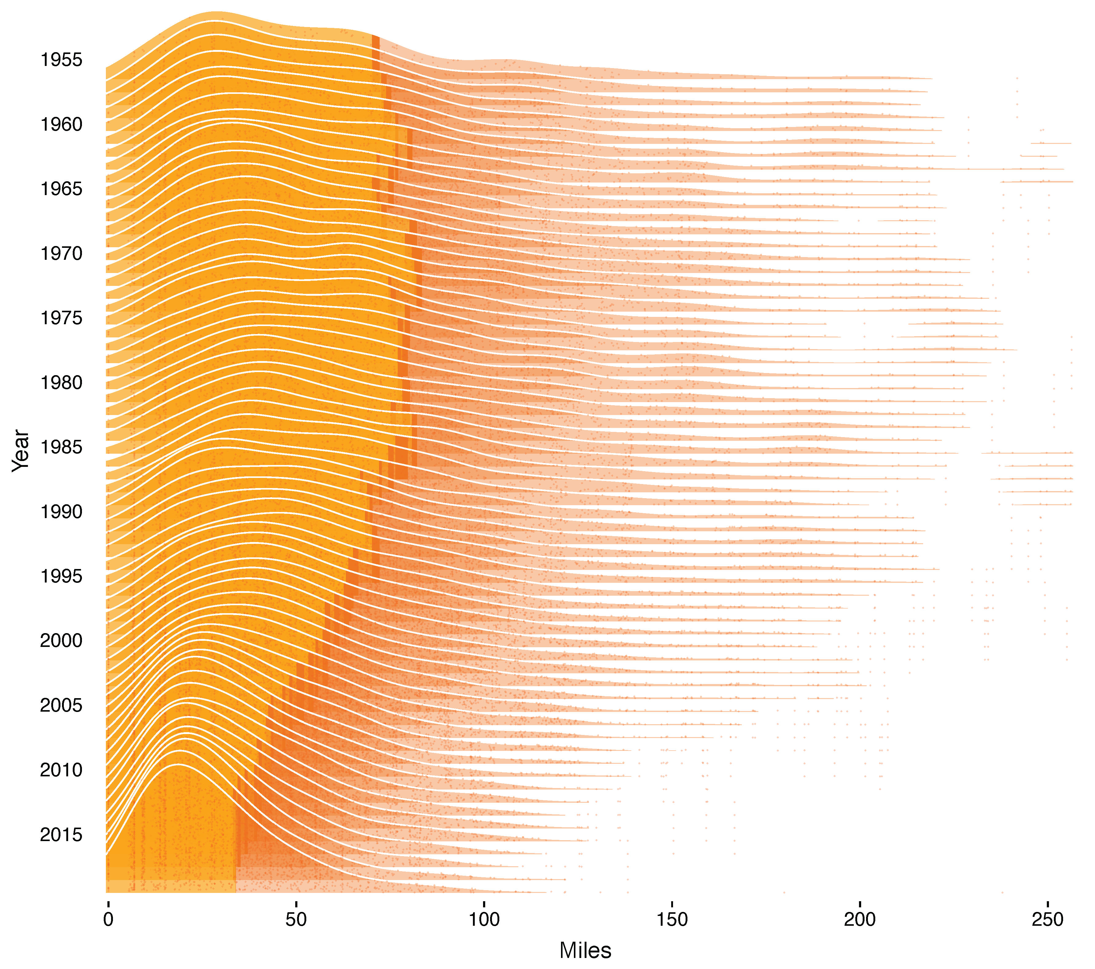
Figure 1 shows how the densities changed over time. Historically they were skewed to the right with long fat tails due to large outliers. Skewness declined dramatically after 1985 and a truncated normal distribution now appears to be a good approximation. Improved accuracy was driven by the use of satellites and supercomputers; see Rappaport et al. (2009).

The 67th percentile of each density is similar to how the NHC measures the radius of the ‘cone of uncertainty’. The radius is measured as the distance that captures 2/3 of all forecast errors in the past five years and denotes the uncertainty associated with the forecast location.3 Thus, I refer to this as the time-varying ex-ante uncertainty.

The most relevant forecasts for hurricane damage are those that are made just before landfall. In total, 88 hurricanes made landfall between 1955 and 2015. Accounting for the fact that some hurricanes struck multiple locations, i.e., Katrina [2005] first crossed the Florida panhandle and then moved into the Gulf and struck Louisiana several days later, there were 101 strikes. I focus on the 98 strikes for which forecasts are available.

Since the forecast and location of the hurricane is only updated at six-hour intervals, I round the timing of each landfall to the closest point in that interval. Therefore, a hurricane landfall at 16:00 Universal Time (UTC) is rounded to 18:00 UTC. I subtract the length of the forecast horizon from the landfall time to get the time at which the 12-hour-ahead ‘landfall forecast’ was generated. So the 12-hour-ahead landfall forecast of a storm that made landfall at 18:00 UTC was generated at 6:00 UTC.

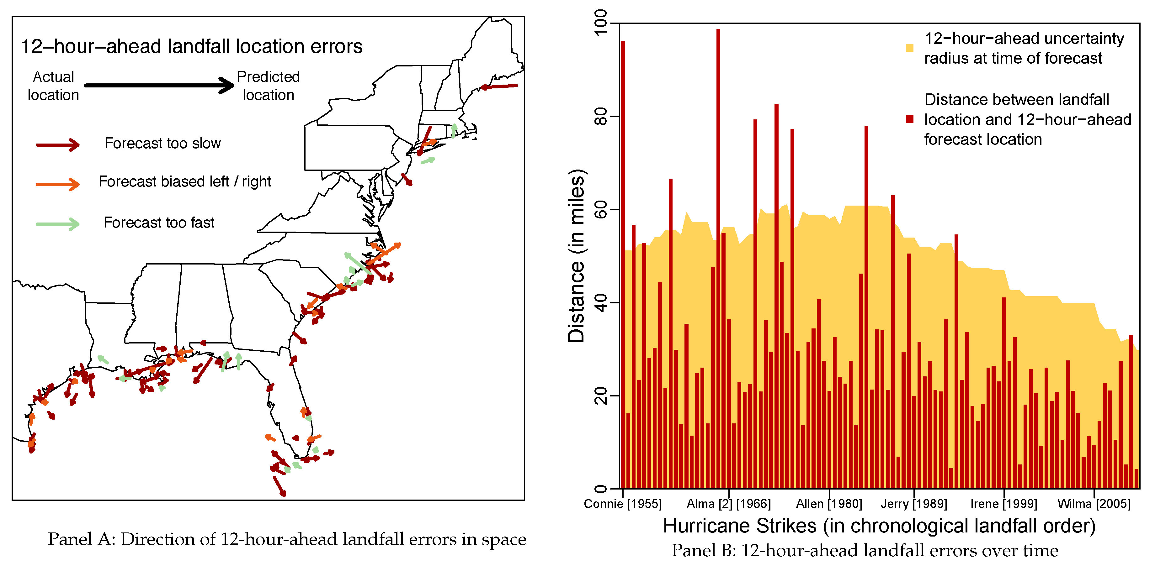
I then compute the landfall forecast error by calculating the distance between the forecast made 12 hours before landfall and the location at landfall. Although the forecast errors are purely distance measures, it is possible to derive forecast error directions based on the location of the hurricane when the forecast was generated. Panel A of Figure 2 plots the spatial distribution of the landfall locations and forecast error directions for most hurricane strikes since 1955. It shows that there is a wide geographic distribution along the Gulf and Atlantic coasts with landfalls ranging from southern Texas to eastern Maine. There also does not appear to be any systematic pattern in the error directions.

Panel B of Figure 2 plots the 12-h-ahead landfall forecast errors for all hurricane strikes along with the estimated ex-ante uncertainty from 1955–2015. The large variation in the forecast errors over time will allow me to identify if they have any impact on damage. Although ex-ante uncertainty has declined gradually since the 1990s, the forecast errors themselves do not have a clear trend despite the fact that larger errors do occur somewhat more often earlier on in the sample. Forecast errors exceed the ex-ante uncertainty in about 12 percent of all strikes; most recently for Sandy [2012].

I collate hurricane strike damage from multiple sources. I primarily rely on annual Atlantic Hurricane Season reports following Pielke and Landsea (1998)4. I supplement and update these numbers using the latest tropical cyclone report for each storm and Blake et al. (2011). The resulting dataset is similar to Pielke et al. (2008). However, it is higher than NOAA’s ‘Storm Events’ database (which suffers from under-reporting; see Smith and Katz 2013) and is somewhat lower than NOAA’s ‘Billion-Dollar’ database, which uses a broader definition of damage; see Weinkle et al. (2018)5.

4. Model Selection Methods

While the relationship between hurricane damage and forecast accuracy is the primary interest of the analysis, there are many other potential determinants of damage. I use model selection to focus the analysis on those variables which are most important for damage. The approach I follow is broadly defined as an automatic general-to-specific (Gets) modeling framework, which is described in detail by Hendry and Doornik (2014). Developments by Hendry et al. (2008), Castle et al. (2012), Castle et al. (2015), Hendry and Johansen (2015) and Pretis et al. (2016), illustrate its usefulness across a range of applications.

The approach starts with the formulation of a general unrestricted model (GUM) that includes all potentially relevant explanatory variables. It is assumed that the residuals of the GUM are iid normal but this can be relaxed in extensions of the framework

$$y_i=\sum _{s=1}^S{\beta }_s{x}_{s,i}+\sum _{n=1}^N{\gamma }_n{z}_{n,i}+{ϵ}_i{ϵ}_i\sim \mathrm{IN}\left[0,{\sigma }_{ϵ}^2\right]\left\{i=1\dots J\right\}.$$

(7)

Theory-driven variables that are not selected over are denoted by $x_s$ and all variables that will be selected over are denoted by $z_n$. It is also assumed that the GUM is potentially sparse and nests the underlying local data generating process (LDGP). This ensures that Gets consistently recovers the same model as if selection began from the LDGP. Thus, formulation of the GUM is an integral part of the modeling process.

The properties of Gets model selection are easily illustrated when each $z_n$ is orthogonal. In this case, selection can be performed by computing the sample of t-statistics under the null hypothesis that $H_0:{\gamma }_n=0\forall n\in N$. The squared t-statistics are then ordered from largest to smallest

$$t_{\left(N\right)}^2\ge \dots \ge t_{\left(m\right)}^2\ge c_a^2\ge t_{(m-1)}^2\ge \dots \ge t_{\left(1\right)}^2,$$

(8)

where $\alpha$ determines the critical value above which variables are retained. In this setup the decision to select is only made once, i.e., ‘one-cut’. Under the null hypothesis, the average number of irrelevant variables retained is

$$k=\sum _{i=0}^{N}i\frac{N!}{i!\left(N-i\right)!}{\alpha }^i{\left(1-\alpha \right)}^{N-i}=N\alpha ,$$

(9)

which shows that $\alpha$ determines the false-retention rate of variables in expectation, i.e., the ‘gauge’ (Castle et al. 2011; Johansen and Nielsen 2016). The gauge plays the same role as regularization does in other machine learning or model selection procedures in that it controls the loss of information in the selection procedure; see Mullainathan and Spiess (2017). However, unlike other regularization parameters which are determined based on in-sample model performance, the gauge has a theoretical interpretation and is typically chosen based on the size of the GUM, $\alpha =1/N$, so that on average one irrelevant variable is kept.

If the variables are correlated then ‘one-cut’ selection is no longer appropriate. However, the approach can be extended by sampling different blocks of variables at a time and ensuring that any reduction satisfies the ‘encompassing principle’ as determined by the gauge; see Doornik (2008). This can be augmented with a multi-path tree search and diagnostic tests so as to minimize potential path dependencies and to ensure a statistically well-specified model; see Hendry and Doornik (2014).

The final model provides a parsimonious explanation of the GUM conditional on the acceptable amount of information loss as determined by the gauge. When multiple models are retained then information criteria are used to select between otherwise equally valid models. Alternatively, ‘thick modeling’, as proposed by Granger and Jeon (2004) and discussed in a Gets framework by Castle (2017), can be used to pool selected models.

There are many different model selection algorithms available. I use the multi-path block search algorithm known as ‘Autometrics’ available in PcGive; see Doornik (2009) and Doornik and Hendry (2013). An alternative multi-path search algorithm is implemented using the ‘gets’ package in R; see Pretis et al. (2018). I also compare the results by performing model selection using regularized regression methods (i.e., Lasso) as implemented in the ‘glmnet’ package in R; see Friedman et al. (2010).

5. Selecting a Model of Damage

The GUM that I estimate includes most potential determinants of hurricane damage and several controls for spatial and temporal heterogeneity. It contains 37 explanatory variables and is estimated over a sample of 98 observations. Lower case variables are in logs:

$$\begin{array}{ccc}{\mathrm{damage}}_i\hfill & =& \begin{array}{c}\hfill c\end{array}+\begin{array}{c}\hfill {\alpha }_1\end{array}{\mathrm{hd}}_i+\begin{array}{c}\hfill {\alpha }_2\end{array}{\mathrm{ih}}_i+\begin{array}{c}\hfill {\alpha }_3\end{array}{\mathrm{FREQ}}_i+\begin{array}{c}\hfill {\beta }_1\end{array}{\mathrm{rain}}_i+\begin{array}{c}\hfill {\beta }_2\end{array}{\mathrm{surge}}_i+\begin{array}{c}\hfill {\beta }_3\end{array}{\mathrm{press}}_i\hfill \\ & +& \begin{array}{c}\hfill {\beta }_4\end{array}{\mathrm{wind}}_i+\begin{array}{c}\hfill {\beta }_5\end{array}{\mathrm{MOIST}}_i+\begin{array}{c}\hfill {\beta }_6\end{array}{\mathrm{ace}}_i+\begin{array}{c}\hfill {\beta }_7\end{array}{\mathrm{GST}}_i+\begin{array}{c}\hfill {\eta }_1\end{array}{\mathrm{forc}12}_i+\begin{array}{c}\hfill {\eta }_2\end{array}{\mathrm{radii}12}_i\hfill \\ & +& \begin{array}{c}\hfill {\delta }_1\end{array}{\mathrm{STREND}}_i+\begin{array}{c}\hfill {\delta }_2\end{array}{\mathrm{YTREND}}_i+\begin{array}{c}\hfill \psi \end{array}{\mathrm{MONTH}}_i+\begin{array}{c}\hfill \kappa \end{array}{\mathrm{HOUR}}_i+\begin{array}{c}\hfill \lambda \end{array}{\mathrm{STATE}}_i+{ϵ}_i.\hfill \end{array}$$

(10)

The first line includes the vulnerabilities (V): housing unit density (hd), income per housing unit (ih) and ‘real-time’ hurricane strike location frequency (FREQ). The first two lines list the natural hazards (F): maximum rainfall (rain), storm surge (surge), negative minimum central pressure (press), maximum wind speed (wind), soil moisture relative to trend (MOIST), accumulated cyclone energy (ace) and global surface temperature (GST).6 The second line captures forecast accuracy and uncertainty (U): 12-hour-ahead forecast track errors (forc12) and the ex-ante uncertainty (radii12). The last line lists additional spatial and temporal controls: strike and annual trends, month dummies, hour dummies (to control for the six-hour period in which the landfall occurred), and U.S. state dummy variables. See Appendix B for further details on how the additional variables were constructed.

I use Gets model selection to discover the most important drivers of hurricane damage without selecting over forecast accuracy and uncertainty. Since the GUM has 35 variables to select over, I set the target gauge equal to $\frac{1}{35}\approx 0.03$. There are $2^{35}$ (>34 billion) possible model combinations when allowing for every variable to be selected over. For a target gauge of 3 percent, the selection algorithm narrows the search space to $2^{17}$ (<200 thousand). It eliminates entire branches of models and ultimately only estimates 304 candidate models. The algorithm finds 8 terminal models as acceptable reductions of the GUM; see Appendix A

Table A1. Estimated Terminal Models for a Gauge of 3%.

Terminal Model:	Final GUM	(1)	(2)	(3)	(4)	(5)	(6)	(7)	(8)
Housing density	0.50 **	0.58 ***	0.49 ***	0.59 ***	0.56 ***	0.64 ***	0.40 ***	0.70 ***	0.55 ***
	(0.19)	(0.14)	(0.15)	(0.14)	(0.14)	(0.18)	(0.15)	(0.18)	(0.14)
Income per household	0.85					1.17 ***	1.30 ***	1.10 ***
	(0.62)					(0.20)	(0.20)	(0.21)
Historical fequency	−5.64 **		−4.85 *	−5.18 **		−6.47 ***		−5.49 **	−5.05 **
	(2.55)		(2.47)	(2.26)		(2.28)		(2.44)	(2.23)
Max rainfall	0.62 *	1.12 ***			1.15 ***		1.15 ***
	(0.37)	(0.32)			(0.32)		(0.31)
Max storm surge	1.15 ***	1.44 ***		1.45 ***	1.42 ***	1.40 ***	1.34 ***	1.35 ***	1.24 ***
	(0.41)	(0.38)		(0.39)	(0.38)	(0.38)	(0.38)	(0.38)	(0.40)
Min central pressure (-)	60.2 ***	53.9 ***	80.4 ***	53.2 ***	67.2 ***	50.8 ***	52.2 ***	65.5 ***	54.2 ***
	(14.0)	(8.66)	(13.3)	(8.90)	(13.5)	(8.59)	(8.58)	(14.1)	(8.79)
Max wind speed	−1.02		−0.92		−1.50			−1.32
	(1.16)		(1.22)		(1.12)			(1.20)
Seasonal cyclone energy	0.43 *			0.60 **		0.58 **			0.64 **
	(0.25)			(0.26)		(0.25)			(0.25)
Soil Moisture	0.67		2.27 **
	(1.00)		(0.93)
Year trend	0.12		−0.07 ***		−0.08 ***				−0.07 ***
	(0.10)		(0.01)		(0.01)				(0.01)
Strike trend	0.09	0.05 ***		0.05 ***
	(0.06)	(0.01)		(0.01)
AUG	0.48		0.47
	(0.36)		(0.39)
SEP	0.22		0.48
	(0.33)		(0.35)
NY	-0.96					−1.79 **		−2.23 ***
	(0.85)					(0.74)		(0.77)
VA	1.66 **		2.09 **						2.14 **
	(0.81)		(0.86)						(0.82)
NC	−0.43		−1.39 ***						−0.80 **
	(0.45)		(0.38)						(0.36)
FL	0.48				0.55 *
	(0.34)				(0.29)
12-h forecast error	0.55 **	0.44 *	0.25	0.33	0.47 *	0.46 *	0.47 *	0.42 *	0.39
	(0.24)	(0.24)	(0.25)	(0.24)	(0.24)	(0.24)	(0.24)	(0.25)	(0.24)
12-h radius	2.34	2.35 *	0.76	2.52 **	1.62	0.44	0.17	−0.04	1.57
	(1.57)	(1.19)	(1.19)	(1.25)	(1.12)	(1.02)	(0.98)	(1.01)	(1.15)
k	17	5	10	6	7	7	5	8	8
Log-likelihood (-)	145.2	157.6	158.4	158.8	156.1	155.0	157.0	157.3	155.1
AIC	3.41	3.42	3.54	3.46	3.43	3.41	3.41	3.48	3.43
HQ	3.65	3.53	3.70	3.58	3.56	3.54	3.52	3.61	3.57
BIC	3.99	3.68	3.93	3.75	3.75	3.73	3.67	3.82	3.77
$\widehat{\sigma }$	1.21	1.27	1.32	1.30	1.27	1.26	1.27	1.29	1.26
$R^2$	0.86	0.82	0.82	0.81	0.82	0.83	0.82	0.82	0.83

Notes: Estimated using 98 observations and include a constant and dummy variables for Gerda [1969] and Floyd [1987]. Each terminal model is selected from the Final GUM using a gauge of 3%. Bolded values indicate terminal models with the lowest information criteria. The standard errors are in parentheses. k is the number of selected regressors. * p < 0.1, ** p < 0.05, *** p < 0.01.

. The final model is selected from the terminal models using the Bayesian information criterion (BIC).

Column (1) of

Table 1. Selected Models of Hurricane Damage.

	(1) Gets	(2) Lasso	(3) Robust Gets
Selection Target:	3%	BIC (9%)	1%
Housing density	0.40 ***	0.40 ***	0.24 **
	(0.15)	(0.15)	(0.09)
Income per housing unit	1.30 ***	1.30 ***	1.76 ***
	(0.20)	(0.20)	(0.19)
Historical frequency		−3.38
		(2.20)
Max rainfall	1.15 ***	0.96 ***	0.56 ***
	(0.31)	(0.32)	(0.20)
Max storm surge	1.34***	1.36***	0.98***
	(0.38)	(0.37)	(0.24)
Min central pressure (-)	52.2 ***	50.2 ***	57.8 ***
	(8.58)	(8.45)	(5.41)
Seasonal cyclone energy		0.57 **
		(0.24)
Forecast errors	0.47 *	0.48 **	0.27 *
	(0.24)	(0.24)	(0.15)
Ex-ante uncertainty	0.17	0.78	2.10 **
	(0.98)	(1.00)	(0.96)
Outliers:	No	No	Yes
Nonlinear terms:	No	No	Yes
$\widehat{\sigma }$	1.268	1.233	0.795
$R^2$	0.821	0.834	0.930
BIC	3.673	3.688	2.774

Notes: 98 observations. Includes a constant and dummy variables for Gerda [1969] and Floyd [1987]. Standard errors are in parentheses. * p < 0.1, ** p < 0.05, *** p < 0.01.

illustrates the most important drivers of damage using Gets. Wind speed does not appear. Instead, minimum central pressure is included. Even when wind speed is included in the model with central pressure, see Appendix A Table A1, the estimated coefficient is the wrong sign. This is consistent with Bakkensen and Mendelsohn (2016), who find that central pressure provides a more reliable explanation of damage. I find more disaggregated measures of hazards with rainfall and storm surges: rainfall causes inland flooding whereas storm surges damage the coast. I also find that greater housing density and higher incomes are associated with more damage.

The results change with other selection methods. Lasso shrinks the estimated coefficients using a penalty, which is chosen here using BIC. The post-selection OLS coefficients (and standard errors) are shown in column (2). All of the variables retained by Gets are also retained by Lasso. However, an additional hazard and a proxy for long-term adaptation are both kept, which is consistent with the fact that BIC corresponds to a looser target gauge of 9 percent for the given sample size and number of variables; see Campos et al. (2003).

To account for possible model misspecification and to assess the robustness of the selected model, I extend the Gets model by selecting over strike fixed effects to capture outliers relative to the model using impulse indicator saturation (IIS; see Hendry et al. 2008; Johansen and Nielsen 2016) and over squares of the explanatory variables to capture potential non-linearities. I find a non-linear relationship between income and damage; which is consistent with Geiger et al. (2016). I also find multiple outlying strikes which capture measurement issues in the 1950s as well as glancing landfalls; see Appendix A

Table A2. A Robust Model of Hurricane Damage.

	(1) Gets (3%)	(3) Extension (1%)	(4) Robust
Housing density	0.40 ***	0.26 **	0.24 **
	(0.15)	(0.10)	(0.09)
Income per housing unit	1.30 ***	1.71 ***	1.76 ***
	(0.20)	(0.21)	(0.19)
Max rainfall	1.15 ***	0.54 **	0.56 ***
	(0.31)	(0.21)	(0.20)
Max storm surge	1.34 ***	0.95 ***	0.98 ***
	(0.38)	(0.25)	(0.24)
Min central pressure (-)	52.2 ***	56.4 ***	57.8 ***
	(8.58)	(5.61)	(5.41)
Forecast errors	0.47 *	0.26	0.27 *
	(0.24)	(0.16)	(0.15)
Ex-ante Uncertainty	0.17	1.94 *	2.10 **
	(0.98)	(1.06)	(0.96)
Income per housing unit sq.		0.65 ***	0.44 ***
		(0.14)	(0.09)
Outlying storms:			-3.19 ***
			(0.35)
Helene [1958]		−2.59 ***
		(0.85)
Cindy [1959]		−4.09 ***
		(0.85)
Gracie [1959]		−2.61 ***
		(0.83)
Alma [1] [1966]		−4.28 ***
		(0.83)
Bret [1999]		−2.45 ***
		(0.85)
Alex [2004]		−3.20 ***
		(0.84)
Arthur [2014]		−3.36 ***
		(0.98)
$\widehat{\sigma }$	1.267	0.804	0.795
$R^2$	0.821	0.934	0.930
${\chi }_{nd}^2\left(2\right)$	7.93 **	0.43	0.65
	[0.019]	[0.806]	[0.722]
$F_{Het}$	2.00 **	1.27	0.87
	[0.028]	[0.237]	[0.617]
$F_{Het-X}$	1.37	0.92	0.81
	[0.139]	[0.615]	[0.769]
$F_{RESET23}$	1.40	1.40	1.51
	[0.253]	[0.253]	[0.226]

Notes: All equations are estimated using 98 observations and include a constant and dummy variables for Gerda [1969] and Floyd [1987]. The standard errors are in parentheses. The diagnostic tests are the ${\chi }_{nd}^2\left(2\right)$ test for non-Normality (Doornik and Hansen 2008), the $F_{Het}$ / $F_{Het-X}$ test for residual heteroskedasticity (with and without cross products; White 1980), and the $F_{RESET23}$ test for incorrect model specification (Ramsey 1969). The tail probability associated with the null hypothesis of each diagnostic test statistic is in square brackets. Income per housing unit is demeaned to facilitate interpretability of the coefficients. * p < 0.1, ** p < 0.05, *** p < 0.01.

. Since the outliers are all negative and roughly the same magnitude, I combine them into a single dummy variable to obtain a more parsimonious model presented in column (3).

Forecast accuracy is significant across the different models. In each case an increase in the errors is associated with an increase in damage even after controlling for ex-ante uncertainty. To put their relative importance into context, the standardized coefficients from the Robust Gets model indicate that it takes roughly a 5 standard deviation shock for forecast errors to have the same impact on hurricane damage as a 1 standard deviation shock to central pressure. This is roughly the same size that is required for rainfall. A simple back of the envelope calculation indicates that, on average, a one standard deviation reduction in the distance between where a hurricane is expected to strike and where it actually strikes is associated with a decline in damage by up to $9000 in per affected household. This represents about 18 percent of the typical insurance claim or about 4 percent of the total replacement value of a typical at risk home in 20187.

Next I consider how sensitive the results are to alternative measures of forecast accuracy and uncertainty.

Table 2. Sensitivity to Measures of Accuracy and Uncertainty.

	(1) Errors	(2) Errors/Radius	(3) R&S (2015)	(4) RMSE
Housing density	0.27 ***	0.28 ***	0.28 ***	0.26 ***
	(0.10)	(0.10)	(0.10)	(0.10)
Income per housing unit	1.43 ***	1.36 ***	1.36 ***	1.44 ***
	(0.12)	(0.12)	(0.12)	(0.13)
Min central pressure (-)	56.6 ***	56.8 ***	56.9 ***	57.3 ***
	(5.49)	(5.55)	(5.58)	(5.51)
Max rainfall	0.57 ***	0.55 ***	0.54 **	0.56 ***
	(0.21)	(0.21)	(0.21)	(0.21)
Max storm surge	0.99 ***	0.97 ***	0.97 ***	0.95 ***
	(0.24)	(0.25)	(0.25)	(0.24)
Forecast errors	0.34 **
	(0.15)
Errors/ex-ante		0.29 *
		(0.16)
Uncertainty			0.23 *
			(0.14)
Weighted RMSE				0.37 *
				(0.19)
Outliers:	Yes	Yes	Yes	Yes
Nonlinear terms:	Yes	Yes	Yes	Yes
$\widehat{\sigma }$	0.812	0.819	0.822	0.817
$R^2$	0.927	0.925	0.925	0.926
BIC	2.781	2.799	2.806	2.795

Notes: All equations are estimated using 98 observations and include a constant and a dummy variable for Gerda [1969] and Floyd [1987]. Standard errors are in parentheses. R&S(2015): Rossi and Sekhposyan (2015). RMSE is weighted using an AR(1) coefficient of 0.3 on forecast errors after the initial strike. * p < 0.1, ** p < 0.05, *** p < 0.01.

presents the results. Column (1) presents a restricted robust gets model which excludes ex-ante uncertainty. Column (2) presents a theory consistent restriction of the robust gets model by imposing a fixed relationship between the forecast errors and the radius of uncertainty; see (5). In both cases these restrictions are strongly rejected. Column (3) uses Rossi and Sekhposyan (2015)’s measure of uncertainty in (4) with a non-parametric time-varying forecast-error distribution based on rolling window of the past five years of forecast errors. Column (4) considers a weighted RMSE measure which quickly decays after landfall.

The results in Table 2 indicate that there is a positive and statistically significant link between alternative measures of forecast accuracy or uncertainty and damage. The size of this relationship is fairly stable regardless of which measure of accuracy or uncertainty is considered. Columns (3) and (4) indicate that imposing a normal distribution on the historical forecast errors does not substantially alter the parameter estimate or increase the noise.

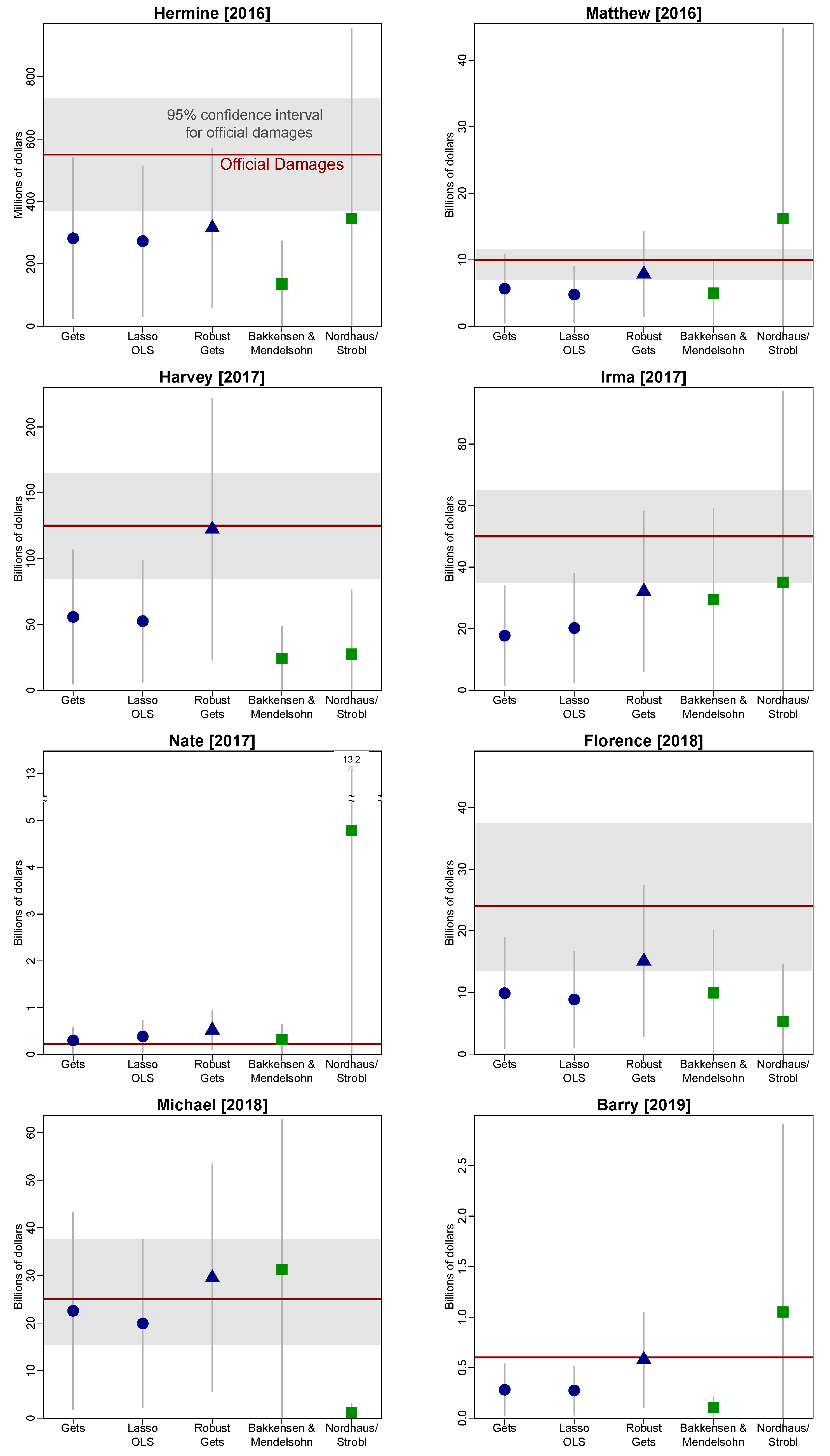
To assess the stability of the models and to ensure that they are not overfitting the data, I evaluate the out-of-sample performance for hurricane strikes between 2016 and 2019. I assess performance relative to two theory-driven models; see Nordhaus (2010) and Strobl (2011) and Bakkensen and Mendelsohn (2016). These models are much simpler in that they only include one natural hazard (central pressure) and one vulnerability (income). To ensure that outliers do not bias the results, I estimate each of these models with a glancing strike dummy variable and without ex-ante uncertainty due to its general insignificance. This ensures that no model has an undue advantage. Thus, the only difference between the Gets and Robust Gets model in this exercise is that the latter includes a non-linear term for income.

Table 3. Relative Out-of-Sample Performance.

	(1) Bias	(2) RMSE	(3) MAPE
Gets	0.91	0.75	0.80
Lasso OLS	0.95	0.77	0.94
Robust Gets	$\mathit{0}.\mathit{20}$	$\mathit{0}.\mathit{20}$	$\mathit{0}.\mathit{64}$
Nordhaus (2010)	1.07	0.99	5.46

Notes: RMSE: Root mean square error. MAPE: Mean absolute percent error. Metrics are computed relative to the performance of the Bakkensen and Mendelsohn (2016) model. Values smaller than 1 indicate better performance.

shows that each of the selected models outperforms the theory-driven models across each of the accuracy metrics. However, the robust model does substantially better than any other model. This is driven by Harvey [2017] where the robust model almost perfectly predicts official damage. However, as Appendix A Figure A1 shows, the robust model consistently outperforms the other models. This suggests that performance is substantially improved when accounting for the non-linear effect of income. It also shows that the models are robust without overfitting the data.

6. Measuring the Impact of Forecast Accuracy

I now consider three different approaches for identifying the impact of forecast accuracy on hurricane damage. The first considers inference in the context of model selection and confirms the above findings. The second treats the selected model as a possibly misspecified structural equation and uses instruments to address concerns of omitted variable bias and endogeneity. The third approach tests for the existence of a causal relationship using model invariance and allows me to perform counterfactual exercises. Together these approaches provide a holistic view of the impact of forecast accuracy on hurricane damage.

6.1. Post-Selection Inference

While model selection is typically used for prediction, it can also be used for inference. However, when conducting inference on selected variables it is important to account for uncertainty in the selection procedure by adjusting the standard errors or critical values; see Berk et al. (2013) and Van de Geer et al. (2014). Alternatively, it is possible to restrict selection such that the variables of interest for inference are always retained and so does not require other adjustments; see Chernozhukov et al. (2018). The results in Table 1 implicitly follow this latter approach since neither forecast errors nor ex-ante uncertainty were selected over. However, the results do not account for correlation between the variables forced in the model and those that were selected over. Therefore, I consider two procedures that control for these correlations and allow for valid inference.

The first approach is to orthogonalize the variables that will be selected over by the variables that will not. This procedure was proposed by Hendry and Johansen (2015) to test the significance of theory relevant variables after performing model selection. I orthogonalize all other variables by forecast accuracy, ex-ante uncertainty and income, which ensures that the relationship between income and damage is not falsely attributed to the relationship between forecast accuracy and damage.

The results are presented in column (1) of

Table 4. The Impact of Forecast Accuracy on Damage.

	(1) Orthogonal Gets	(2) Double Lasso	(3) IV
Selection Target:	3%	BIC (9%)
Forecast errors	0.39 *	0.50 **	0.49 ***
	(0.23)	(0.21)	(0.17)
Ex-ante Uncertainty	−1.58	0.98	2.95 **
	(1.13)	(1.01)	(1.25)
Obs.	98	98	65

Notes: HAC standard errors are in parentheses: * p < 0.1, ** p < 0.05, *** p < 0.01.

. The selected variables are identical to the previous Gets result in Table 1; however the coefficients on forecast errors and ex-ante uncertainty are different. The coefficient for forecast errors is slightly smaller but remains statistically significant at the 10% level. On the other hand, the coefficient on ex-ante uncertainty is now negative but is not statistically significant from zero. This illustrates that the correlations between variables play an important role when interpreting the results for ex-ante uncertainty.

The second approach is a double Lasso procedure whereby variables that explain forecast accuracy or uncertainty are retained regardless of whether they matter for damage. This was proposed by Belloni et al. (2014) in the context of treatment variables in order to protect against omitted variable bias due to selection. The procedure is described as follows: Run a Lasso regression on the full model of damage excluding forecast accuracy and ex-ante uncertainty. Next, run a Lasso regression for the models of forecast accuracy and ex-ante uncertainty using all other explanatory variables. Finally, combine the variables selected in the first two stages along with forecast errors and ex-ante uncertainty into an OLS regression on damage. This allows for valid inference on the forecast errors and ex-ante uncertainty when they are conditionally exogenous.

The results for these two coefficients are shown in column (2) of Table 4. The coefficient for forecast errors is different from zero at a 5% significance level and is broadly consistent with the results in column (1) and those in Table 1. On the other hand, the coefficient on ex-ante uncertainty is positive and statistically insignificant.

6.2. Exogenous Instruments

The post-selection inference approaches assume that forecast errors and ex-ante uncertainty are exogenous conditional on the other explanatory variables in the GUM. However, if this assumption does not hold, then these procedures will produce biased estimates of the true parameters. Therefore, it is important to include additional variables in the model or to use of an exogenous instrument to ensure that this assumption is not violated.

There are several reasons why the forecast errors may not be exogenous. Errors may be correlated with storm dynamics where a volatile storm that is more difficult to forecast causes more damage. For example, the rapid intensification of a hurricane prior to landfall is difficult to forecast and is associated with higher damage; see Kaplan et al. (2010). Errors may be correlated with long-term adaptation and technological change. This is especially true when considering that the measure of ex-ante uncertainty is effectively a five-year moving percentile of forecast errors and so is driven more by longer-term trends such as government expenditures and technological change. Both of these effects could bias the estimated relationship between forecast accuracy and damage.

I construct an instrument based on a measure of forecast skill in order to address concerns about storm dynamics. Forecast skill is often used to assess the performance of hurricane and weather forecasts over time; see Cangialosi and Franklin (2016). I calculate forecast skill as the inverse ratio of the official forecast errors to naïve forecast errors from a simple climatology and persistence model (available since 1970). As a result, forecasts for an erratic storm that is more difficult to forecast will not be penalized with lower skill. Assuming that both types of forecast errors are log normal and affected in the same way by the endogenous storm dynamics, then the log forecast skill is a valid instrument by removing the endogeneity.

I also include several additional controls. To control for longer-term adaptation efforts I include the normalized length of protective levees from the US Army Corps of Engineers’ National Levee Database as a measure of how location-specific adaptation efforts changed over time. To control for the role of hurricane evacuations I use hurricane warning lead times. Earlier warnings are given for stronger storms or when they are expected to strike more populated locations. Earlier warning times can also cover larger areas due to the uncertainty associated with the path of the hurricane. I address this by looking at the number of hours in advance a warning was given to the eventual landfall location divided by the length of coastline under warning.

I perform two-stage least squares starting from the robust Gets model with the additional controls. Forecast skill is highly significant in the first stage regression with a t-value of −7.4. Table 4 shows the second stage estimates for the instrumented forecast errors and ex-ante uncertainty. The coefficient on instrumented forecast errors is highly significant at a 1% level and is similar in magnitude to the other estimates despite being based on a smaller sample starting in 1970. Ex-ante uncertainty remains positive and is different from zero at a 5% significance level. Thus, the results from this exercise suggest that the findings are robust to additional controls and accounting for endogeneity concerns.

6.3. Model Invariance and Valuing Improved Forecast Accuracy

Another approach is to identify causal relationships through model invariance; see Engle et al. (1983), Peters et al. (2016), and Arjovsky et al. (2019). The idea behind this is that if historical shocks to forecast errors only impact damage through forecast errors, then the model of damage is invariant to changes in the forecast errors and there is a likely causal relationship between forecast errors and damage; see Hendry (1995, chp. 5). Several tests of model invariance were proposed in the time-series literature by Engle and Hendry (1993), Hendry and Santos (2010), and Castle et al. (2017).

To test the invariance of the robust Gets model with respect to the forecast errors, I follow the approach in Hendry and Santos (2010). First, I run impulse indicator saturation (IIS) on the marginal model of forecast errors regressed on all other explanatory variables. I retain any impulses detected in this model. Next, I estimate the conditional model of damage regressed on the forecast errors, all other explanatory variables, and the retained impulses from the marginal model. Finally, I test the joint significance of these impulses in the conditional model. The null hypothesis is that the model is invariant so that any shocks to the marginal model pass directly through the forecast errors to damage and do not otherwise change the parameters of the conditional model.

Table 5. A Test of Model Invariance.

	(1) Marginal + IIS	(2) Augmented Conditional
Retained Impulses:	Forecast Errors	Damage
Connie [1955]	1.29 (0.57) **	−0.96 (0.96)
Cleo [1964]	−1.21 (0.51) **	1.38 (0.87)
Opal [1995]	−1.48 (0.52) ***	0.24 (0.89)
Isabel [2003]	−1.19 (0.50) **	0.98 (0.85)
Arthur [2014]	−1.73 (0.54) ***	−0.53 (0.94)
F-statistic		1.05
p-value		[0.394]

Notes: Estimated using 98 observations with all regressors from the Robust Gets model. IIS is run using a 1% gauge. Standard errors are in parentheses. The tail probability associated with the null hypothesis of the F-statistic with (5,83) degrees of freedom is in square brackets. * p < 0.1, ** p < 0.05, *** p < 0.01.

shows that five outlying storms are detected in the marginal equation for forecast errors: Connie [1955], Cleo [1964], Opal [1995], Isabel [2003] and Arthur [2014]. However, after adding them to the conditional model and testing for their joint significance, a test statistic of $1.05$ is obtained which when compared against an F-distribution with (5, 83) degrees of freedom indicates that the null hypothesis of model invariance is not rejected with a p-value of $39.4$ percent. This suggests that there is a causal relationship between the forecast errors and hurricane damage in this model.

The robust Gets model can also be used to conduct counterfactual experiments to assess the short-term impact of changes in forecast accuracy on hurricane damage. This requires that the parameter linking forecast accuracy to hurricane damage is identified such that model is semi-structural. The relative stability of the parameter estimate across different approaches and the failure to reject model invariance when there are large shocks to the forecast errors all suggest that the true parameter is identified. Assuming this is true, then the robust Gets model can be used to predict damage conditional on the forecast error for each strike since 1970 being equal to the average landfall-forecast error from 1955–1969. The model can also be used to predict damage conditional on the actual forecast error. The difference between these predictions is a prediction of the damage prevented due to forecast improvements since 1970. Under additional independence and normality assumptions it is possible construct a 95 percent point-wise confidence interval around this prediction8.

Figure 3 shows that the cumulative damage prevented due to forecast improvements since 1970 was around $\$82$ billion in 2015. This is about 14 percent of the total predicted damage from 1970–2015 and is just shy of the total damage caused by Maria [2018]. It is driven both by improvements in forecast accuracy and by more damaging storms. Damage prevented is most pronounced for the 2005 and 2008 hurricane seasons which saw several very destructive hurricanes and above average forecast accuracy. On the other hand, despite the destructiveness of Sandy [2012], there was little damage prevented as the forecasts were not substantially different from the pre-1970 average.

To assess the relative benefits, I compare the prediction against two different estimates of costs. The first is the range of cumulative costs of producing the forecasts and their improvements since 19709. After accounting for these costs, the predicted net savings is around $30–71 billion. The second measure of cost is the cumulative private willingness to pay for forecast improvements since 1970 as extrapolated from Katz and Lazo (2011). The benefits of forecast improvements are greater than both public spending and private willingness to pay for them. This suggests that both individuals and the U.S. federal government underestimate the value of improving hurricane forecasts. This estimate is a lower bound of the total net benefits from forecast improvements since fatalities prevented (Willoughby et al. 2007) and reduced evacuation and damage mitigation costs (Regnier 2008) are excluded.

7. Conclusions

In this paper I evaluate the relationship between forecast accuracy and hurricane damage using a model of damage for all hurricanes to strike the continental United States in the past 60 years. I start with many possible drivers of damage and use model selection methods to determine the most important ones. I show that a small sub-set of drivers explains most of the historical damage and performs well for the latest hurricane strikes.

Despite specifying a richer model than previous studies, I find that forecast accuracy matters for damage. This relationship is positive, statistically significant and is robust to outliers, alternative measures of accuracy, model specifications, out-of-sample storms, and additional controls. On average, a one standard deviation increase in the distance between the storm’s predicted and actual landfall location translates on average into roughly $\$9000$ additional dollars in damage per affected household. This value is equivalent to about 18 percent of the typical flood insurance claim or four percent of the total replacement value of a typical home at risk of hurricane damage in 2018.

Using a counterfactual exercise, I show that improvements in the forecasts since 1970 resulted in total damage being approximately $\$82$ billion less than it otherwise would have been. Although damage increased due to changes in vulnerabilities and natural hazards, improvements in forecast accuracy along with longer-term adaptation efforts have kept it from rising faster than it otherwise would have. I find that there is a net benefit of around $30–71 billion when compared against the cost of producing the forecasts. This illustrates that improvements in the forecasts produce benefits beyond the well-documented reduction in fatalities and outweighed the associated costs.

This is particularly important since hurricanes are expected to become more difficult to forecast in the future. Knutson et al. (2010) argue that climate change will increase hurricane intensity and there will be more hurricanes, such as Harvey [2017], whose dynamics are hard to predict (Emanuel 2017a, 2017b). In light of this reality, these findings support maintained investment in and further measures to improve hurricane forecasting capabilities along with other longer-term adaptation efforts so that any future loss of life and property is minimal.

References

- Arjovsky, Martin, Léon Bottou, Ishaan Gulrajani, and David Lopez-Paz. 2019. Invariant risk minimization. arXiv arXiv:1907.02893. [Google Scholar]
- Bakkensen, Laura A., and Robert O. Mendelsohn. 2016. Risk and adaptation: Evidence from global hurricane damages and fatalities. Journal of the Association of Environmental and Resource Economists 3: 555–87. [Google Scholar] [CrossRef] [Green Version]
- Beatty, Timothy K. M., Jay P. Shimshack, and Richard J. Volpe. 2019. Disaster preparedness and disaster response: Evidence from sales of emergency supplies before and after hurricanes. Journal of the Association of Environmental and Resource Economists 6: 633–68. [Google Scholar] [CrossRef]
- Belloni, Alexandre, Victor Chernozhukov, and Christian Hansen. 2014. Inference on treatment effects after selection among high-dimensional controls. The Review of Economic Studies 81: 608–50. [Google Scholar] [CrossRef]
- Berk, Richard, Lawrence Brown, Andreas Buja, Kai Zhang, and Linda Zhao. 2013. Valid post-selection inference. The Annals of Statistics 41: 802–37. [Google Scholar] [CrossRef] [Green Version]
- Blake, Eric S., Edward N. Rappaport, and Christopher W. Landsea. 2011. The Deadliest, Costliest, and Most Intense United States Tropical Cyclones from 1851 to 2010 (and Other Frequently Requested Hurricane Facts). Silver Spring: NOAA, National Weather Service, National Centers for Environmental Prediction, National Hurricane Center. [Google Scholar]
- Broad, Kenneth, Anthony Leiserowitz, Jessica Weinkle, and Marissa Steketee. 2007. Misinterpretations of the “Cone of Uncertainty” in Florida during the 2004 hurricane season. Bulletin of the American Meteorological Society 88: 651–67. [Google Scholar] [CrossRef]
- Campos, Julia, David F. Hendry, and Hans-Martin Krolzig. 2003. Consistent model selection by an automatic gets approach. Oxford Bulletin of Economics and Statistics 65: 803–19. [Google Scholar] [CrossRef]
- Cangialosi, John P., and James L. Franklin. 2016. 2015 Hurricane Season. In NHC Forecast Verification Report. Silver Spring: NOAA (National Hurricane Center). [Google Scholar]
- Castle, Jennifer L. 2017. Sir Clive WJ Granger Model Selection. European Journal of Pure and Applied Mathematics 10: 133–56. [Google Scholar]
- Castle, Jennifer L., Jurgen A. Doornik, and David F. Hendry. 2011. Evaluating automatic model selection. Journal of Time Series Econometrics 13: 1–31. [Google Scholar] [CrossRef] [Green Version]
- Castle, Jennifer L., Jurgen A. Doornik, and David F. Hendry. 2012. Model selection when there are multiple breaks. Journal of Econometrics 169: 239–46. [Google Scholar] [CrossRef] [Green Version]
- Castle, Jennifer L., Jurgen A. Doornik, David F. Hendry, and Felix Pretis. 2015. Detecting location shifts during model selection by step-indicator saturation. Econometrics 3: 240–64. [Google Scholar] [CrossRef] [Green Version]
- Castle, Jennifer L., David F. Hendry, and Andrew B. Martinez. 2017. Evaluating forecasts, narratives and policy using a test of invariance. Econometrics 5: 39. [Google Scholar] [CrossRef] [Green Version]
- Chavas, Daniel R., Kevin A. Reed, and John A. Knaff. 2017. Physical understanding of the tropical cyclone wind-pressure relationship. Nature Communications 8: 1–11. [Google Scholar] [CrossRef]
- Chernozhukov, Victor, Denis Chetverikov, Mert Demirer, Esther Duflo, Christian Hansen, Whitney Newey, and James Robins. 2018. Double/debiased machine learning for treatment and structural parameters. The Econometrics Journal 21: C1–C68. [Google Scholar] [CrossRef]
- Clements, Michael P. 2014. Forecast uncertainty—Ex Ante and Ex Post: U.S. inflation and output growth. Journal of Business & Economic Statistics 32: 206–16. [Google Scholar]
- Davlasheridze, Meri, Karen Fisher-Vanden, and H. Allen Klaiber. 2017. The effects of adaptation measures on hurricane induced property losses: Which FEMA investments have the highest returns? Journal of Environmental Economics and Management 81: 93–114. [Google Scholar] [CrossRef] [Green Version]
- Dehring, Carolyn A., and Martin Halek. 2013. Coastal Building Codes and Hurricane Damage. Land Economics 89: 597–613. [Google Scholar] [CrossRef]
- DeMaria, Mark, John Knaff, Richard Knabb, Chris Lauer, Charles Sampson, and Robert DeMaria. 2009. A new method for estimating tropical cyclone wind speed probabilities. Weather and Forecasting 24: 1573–91. [Google Scholar] [CrossRef]
- Deryugina, Tatyana. 2017. The Fiscal Cost of Hurricanes: Disaster Aid Versus Social Insurance. American Economic Journal: Economic Policy 9: 168–98. [Google Scholar] [CrossRef] [Green Version]
- Deryugina, Tatyana, Laura Kawano, and Steven Levitt. 2018. The economic impact of hurricane katrina on its victims: Evidence from individual tax returns. American Economic Journal: Applied Economics 10: 202–33. [Google Scholar] [CrossRef] [Green Version]
- Doornik, Jurgen A. 2008. Encompassing and automatic model selection. Oxford Bulletin of Economics and Statistics 70: 915–25. [Google Scholar] [CrossRef]
- Doornik, Jurgen A. 2009. Autometrics. In The Methodology and Practice of Econometrics: A Festschrift in Honour of David F. Hendry. Edited by Neil Shephard and Jennifer L. Castle. Oxford: Oxford University Press, pp. 88–121. [Google Scholar]
- Doornik, Jurgen A., and Henrik Hansen. 2008. An omnibus test for univariate and multivariate normality. Oxford Bulletin of Economics and Statistics 70: 927–39. [Google Scholar] [CrossRef]
- Doornik, Jurgen A., and David F. Hendry. 2013. Empirical Econometric Modelling. Volume I of PcGive 14. Richmond upon Thames: Timberlake Consultants Ltd. [Google Scholar]
- Emanuel, Kerry. 2005. Increasing destructiveness of tropical cyclones over the past 30 years. Nature 436: 686–88. [Google Scholar] [CrossRef]
- Emanuel, Kerry. 2017a. Assessing the present and future probability of hurricane harvey’s rainfall. Proceedings of the National Academy of Sciences 114: 12681–84. [Google Scholar] [CrossRef] [Green Version]
- Emanuel, Kerry. 2017b. Will global warming make hurricane forecasting more difficult? Bulletin of the American Meteorological Society 98: 495–501. [Google Scholar] [CrossRef] [Green Version]
- Engle, Robert F., and David F. Hendry. 1993. Testing superexogeneity and invariance in regression models. Journal of Econometrics 56: 119–39. [Google Scholar] [CrossRef]
- Engle, Robert F., David F. Hendry, and Jean-Francois Richard. 1983. Exogeneity. Econometrica 51: 277–304. [Google Scholar] [CrossRef]
- Ericsson, Neil R. 2001. Forecast uncertainty in economic modeling. In Understanding Economic Forecasts. Edited by David F. Hendry and Neil R. Ericsson. Cambridge: MIT Press chp. 5, pp. 68–92. [Google Scholar]
- Estrada, Francisco, W. J. Wouter Botzen, and Richard S. J. Tol. 2015. Economic losses from US hurricanes consistent with an influence from climate change. Nature Geoscience 8: 880–84. [Google Scholar] [CrossRef]
- Friedman, Jerome, Trevor Hastie, and Rob Tibshirani. 2010. Regularization paths for generalized linear models via coordinate descent. Journal of Satistical Software 33: 1. [Google Scholar] [CrossRef] [Green Version]
- Gallagher, Justin, and Daniel Hartley. 2017. Household finance after a natural disaster: The case of hurricane katrina. American Economic Journal: Economic Policy 9: 199–228. [Google Scholar] [CrossRef] [Green Version]
- Geiger, Tobias, Katja Frieler, and Anders Levermann. 2016. High-income does not protect against hurricane losses. Environmental Research Letters 11: 084012. [Google Scholar] [CrossRef] [Green Version]
- Granger, Clive W. J., and Yongil Jeon. 2004. Thick modeling. Economic Modelling 21: 323–43. [Google Scholar] [CrossRef]
- Hendry, David F. 1995. Dynamic Econometrics. Oxford: Oxford University Press. [Google Scholar]
- Hendry, David F., and Jurgen A. Doornik. 2014. Empirical Model Discovery and Theory Evaluation: Automatic Selection Methods in Econometrics. Cambridge: MIT Press. [Google Scholar]
- Hendry, David F., and Søren Johansen. 2015. Model discovery and Trygve Haavelmo’s legacy. Econometric Theory 31: 93–114. [Google Scholar] [CrossRef] [Green Version]
- Hendry, David F., Søren Johansen, and Carlos Santos. 2008. Automatic selection of indicators in a fully saturated regression. Computational Statistics 23: 337–39. [Google Scholar] [CrossRef] [Green Version]
- Hendry, David F., and Grayham E. Mizon. 2014. Unpredictability in economic analysis, econometric modeling and forecasting. Journal of Econometrics 182: 186–95. [Google Scholar] [CrossRef] [Green Version]
- Hendry, David F., and Carlos Santos. 2010. An Automatic Test of Super Exogeneity. In Volatility and Time Series Econometrics. Edited by Mark W. Watson, Tim Bollerslev and Jeffrey R. Russell. Oxford: Oxford University Press, pp. 164–93. [Google Scholar]
- Hsiang, Solomon M., and Daiju Narita. 2012. Adaptation to cyclone risk: Evidence from the global cross-section. Climate Change Economics 3: 1250011. [Google Scholar] [CrossRef]
- Jarrell, Jerry D., Paul J. Hebert, and Max Mayfield. 1992. Hurricane Experience Levels of Coastal County Populations from Texas to Maine. Silver Spring: US Department of Commerce, National Oceanic and Atmospheric Administration, National Weather Service, National Hurricane Center, vol. 46. [Google Scholar]
- Johansen, Søren, and Bent Nielsen. 2016. Asymptotic theory of outlier detection algorithms for linear time series regression models. Scandinavian Journal of Statistics 43: 321–48. [Google Scholar] [CrossRef] [Green Version]
- Jurado, Kyle, Sydney C. Ludvigson, and Serena Ng. 2015. Measuring uncertainty. The American Economic Review 105: 1177–216. [Google Scholar] [CrossRef]
- Kaplan, John, Mark DeMaria, and John A. Knaff. 2010. A revised tropical cyclone rapid intensification index for the Atlantic and eastern North Pacific basins. Weather and Forecasting 25: 220–41. [Google Scholar] [CrossRef]
- Katz, Richard W., and Jeffrey K. Lazo. 2011. Economic value of weather and climate forecasts. In The Oxford Handbook on Economic Forecasting. Edited by Michael P Clements and David F Hendry. Oxford: Oxford University Press. [Google Scholar]
- Kellenberg, Derek K., and Ahmed Mushfiq Mobarak. 2008. Does rising income increase or decrease damage risk from natural disasters? Journal of Urban Economics 63: 788–802. [Google Scholar] [CrossRef]
- Kidder, Stanley Q., John A. Knaff, Sheldon J. Kusselson, Michael Turk, Ralph R. Ferraro, and Robert J. Kuligowski. 2005. The tropical rainfall potential (TRaP) technique. Part i: Description and examples. Weather and Forecasting 20: 456–64. [Google Scholar] [CrossRef] [Green Version]
- Knutson, Thomas R., John L. McBride, Johnny Chan, Kerry Emanuel, Greg Holland, Chris Landsea, Isaac Held, James P. Kossin, A. K. Srivastava, and Masato Sugi. 2010. Tropical cyclones and climate change. Nature Geoscience 3: 157–63. [Google Scholar] [CrossRef] [Green Version]
- Kruttli, Mathias, Brigitte Roth Tran, and Sumudu W. Watugala. 2019. Pricing Poseidon: Extreme Weather Uncertainty and Firm Return Dynamics. Finance and Economics Discussion Series 2019-054. Washington, DC: Board of Governors of the Federal Reserve System. [Google Scholar]
- Letson, David, Daniel S. Sutter, and Jeffrey K. Lazo. 2007. Economic value of hurricane forecasts: An overview and research needs. Natural Hazards Review 8: 78–86. [Google Scholar] [CrossRef] [Green Version]
- Milch, Kerry, Kenneth Broad, Ben Orlove, and Robert Meyer. 2018. Decision science perspectives on hurricane vulnerability: Evidence from the 2010–2012 atlantic hurricane seasons. Atmosphere 9: 32. [Google Scholar] [CrossRef] [Green Version]
- Mitchell, James, and Kenneth F. Wallis. 2011. Evaluating density forecasts: Forecast combinations, model mixtures, calibration and sharpness. Journal of Applied Econometrics 26: 1023–40. [Google Scholar] [CrossRef] [Green Version]
- Morana, Claudio, and Giacomo Sbrana. 2019. Climate change implications for the catastrophe bonds market: An empirical analysis. Economic Modelling 81: 274–94. [Google Scholar] [CrossRef]
- Mullainathan, Sendhil, and Jann Spiess. 2017. Machine learning: An applied econometric approach. Journal of Economic Perspectives 31: 87–106. [Google Scholar] [CrossRef] [Green Version]
- Murnane, Richard J., and James B. Elsner. 2012. Maximum wind speeds and US hurricane losses. Geophysical Research Letters 39: 1–5. [Google Scholar] [CrossRef] [Green Version]
- National Science Board. 2007. Hurricane Warning: The Critical Need for a National Hurricane Research Initiative; Technical Report NSB-06-115. Alexandria: National Science Foundation.
- NOAA NCEI. 2018. U.S. Billion-Dollar Weather and Climate Disasters. Available online: https://www.ncdc.noaa.gov/billions/ (accessed on 7 September 2018).
- Nordhaus, William D. 2010. The economics of hurricanes and implications of global warming. Climate Change Economics 1: 1–20. [Google Scholar] [CrossRef]
- Peters, Jonas, Peter Bühlmann, and Nicolai Meinshausen. 2016. Causal inference by using invariant prediction: Identification and confidence intervals. Journal of the Royal Statistical Society: Series B (Statistical Methodology) 78: 947–1012. [Google Scholar] [CrossRef]
- Pielke, Roger A., Jr., Joel Gratz, Christopher W. Landsea, Douglas Collins, Mark A. Saunders, and Rade Musulin. 2008. Normalized hurricane damage in the United States: 1900–2005. Natural Hazards Review 9: 29–42. [Google Scholar] [CrossRef]
- Pielke, Roger A., Jr., and Christopher W. Landsea. 1998. Normalized hurricane damages in the United States: 1925-95. Weather and Forecasting 13: 621–31. [Google Scholar] [CrossRef]
- Pretis, Felix, James Reade, and Genaro Sucarrat. 2018. Automated General-to-Specific (GETS) Regression Modeling and Indicator Saturation for Outliers and Structural Breaks. Journal of Statistical Software 86: 1–44. [Google Scholar] [CrossRef]
- Pretis, Felix, Lea Schneider, Jason E. Smerdon, and David F. Hendry. 2016. Detecting Volcanic Eruptions in Temperature Reconstructions by Designed Break-Indicator Saturation. Journal of Economic Surveys 30: 403–29. [Google Scholar] [CrossRef]
- Ramsey, James Bernard. 1969. Tests for specification errors in classical linear least-squares regression analysis. Journal of the Royal Statistical Society. Series B (Methodological) 31: 350–71. [Google Scholar] [CrossRef]
- Rappaport, Edward N., James L. Franklin, Lixion A. Avila, Stephen R. Baig, John L. Beven, Eric S Blake, Christopher A. Burr, Jiann-Gwo Jiing, Christopher A. Juckins, Richard D. Knabb, and et al. 2009. Advances and challenges at the National Hurricane Center. Weather and Forecasting 24: 395–419. [Google Scholar] [CrossRef] [Green Version]
- Ravn, Morten O., and Harald Uhlig. 2002. On adjusting the Hodrick-Prescott filter for the frequency of observations. The Review of Economics and Statistics 84: 371–76. [Google Scholar] [CrossRef] [Green Version]
- Regnier, Eva. 2008. Public evacuation decisions and hurricane track uncertainty. Management Science 54: 16–28. [Google Scholar] [CrossRef]
- Resio, Donald T., Nancy J. Powell, Mary A. Cialone, Himangshu S. Das, and Joannes J. Westerink. 2017. Quantifying impacts of forecast uncertainties on predicted storm surges. Natural Hazards 88: 1423–49. [Google Scholar] [CrossRef]
- Rossi, Barbara, and Tatevik Sekhposyan. 2015. Macroeconomic uncertainty indices based on nowcast and forecast error distributions. American Economic Review: Papers and Proceedings 105: 650–55. [Google Scholar] [CrossRef] [Green Version]
- Rossi, Barbara, Tatevik Sekhposyan, and Matthieu Soupre. 2017. Understanding the Sources of Macroeconomic Uncertainty. Barcelona GSE Working Paper Series No. 920. Barcelona: GSE. [Google Scholar]
- Sadowski, Nicole Cornell, and Daniel Sutter. 2005. Hurricane fatalities and hurricane damages: Are safer hurricanes more damaging? Southern Economic Journal 72: 422–32. [Google Scholar] [CrossRef]
- Shrader, Jeffrey. 2018. Expectations and Adaptation to Environmental Risks. SSRN Working Paper. Available online: https://ssrn.com/abstract=3212073 (accessed on 5 May 2020).
- Smith, Adam B., and Richard W. Katz. 2013. US billion-dollar weather and climate disasters: Data sources, trends, accuracy and biases. Natural Hazards 67: 387–410. [Google Scholar] [CrossRef]
- Strobl, Eric. 2011. The economic growth impact of hurricanes: Evidence from US coastal counties. Review of Economics and Statistics 93: 575–89. [Google Scholar] [CrossRef]
- U.S. Army Corps of Engineers. 2004. Hurricane Assessment Concerns and Recommendations. Available online: https://web.archive.org/web/20090726033748/http://chps.sam.usace.army.mil/USHESdata/Assessments/2004Storms/2004-Recommendations.htm (accessed on 22 December 2017).
- Van de Geer, Sara, Peter Bühlmann, Ya’acov Ritov, and Ruben Dezeure. 2014. On asymptotically optimal confidence regions and tests for high-dimensional models. The Annals of Statistics 42: 1166–202. [Google Scholar] [CrossRef]
- van den Dool, Huug, Jin Huang, and Yun Fan. 2003. Performance and analysis of the constructed analogue method applied to US soil moisture over 1981–2001. Journal of Geophysical Research: Atmospheres 108: 1–16. [Google Scholar] [CrossRef]
- Vincenty, Thaddeus. 1975. Direct and inverse solutions of geodesics on the ellipsoid with application of nested equations. Survey Review 23: 88–93. [Google Scholar] [CrossRef]
- Weinkle, Jessica, Chris Landsea, Douglas Collins, Rade Musulin, Ryan P. Crompton, Philip J. Klotzbach, and Roger Pielke. 2018. Normalized hurricane damage in the continental United States 1900–2017. Nature Sustainability 1: 808. [Google Scholar] [CrossRef]
- White, Halbert. 1980. A heteroskedasticity-consistent covariance matrix estimator and a direct test for heteroskedasticity. Econometrica 48: 817–38. [Google Scholar] [CrossRef]
- Willoughby, Hugh E., E. N. Rappaport, and F. D. Marks. 2007. Hurricane forecasting: The state of the art. Natural Hazards Review 8: 45–49. [Google Scholar] [CrossRef] [Green Version]