Dynamic Panel Modeling of Climate Change

Abstract

We discuss some conceptual and practical issues that arise from the presence of global energy balance effects on station level adjustment mechanisms in dynamic panel regressions with climate data. The paper provides asymptotic analyses, observational data computations, and Monte Carlo simulations to assess the use of various estimation methodologies, including standard dynamic panel regression and cointegration techniques that have been used in earlier research. The findings reveal massive bias in system GMM estimation of the dynamic panel regression parameters, which arise from fixed effect heterogeneity across individual station level observations. Difference GMM and Within Group (WG) estimation have little bias and WG estimation is recommended for practical implementation of dynamic panel regression with highly disaggregated climate data. Intriguingly, from an econometric perspective and importantly for global policy analysis, it is shown that in this model despite the substantial differences between the estimates of the regression model parameters, estimates of global transient climate sensitivity (of temperature to a doubling of atmospheric CO${}_2$) are robust to the estimation method employed and to the specific nature of the trending mechanism in global temperature, radiation, and CO${}_2.$

1. Introduction

A natural and near universal condition in modeling climate is the use of an energy balance relationship that links average global temperature to average global downwelling radiation and greenhouse gas influences. This balance suggests the existence of a long run cointegrating econometric relation among these variables, a relation that is now supported by considerable empirical evidence (Kaufmann et al. 2011, 2013; Storelvmo et al. 2016, 2018). While such global balancing relations are of considerable interest in themselves, they are also useful in the specification of more detailed models that relate to station level behavior and adjustments that must necessarily take global influences into account. Panel models of this type have been used recently in climate studies by Magnus et al. (2011) and Storelvmo et al. (2016). These studies help to assess, inter alia, the impact that atmospheric aerosols have on measurements of greenhouse gas (GHG) effects on global warming and thereby the measurement of transient climate sensitivity (TCS) to CO${}_2,$ which is arguably the ‘holy grail’ of modern climate science. These econometric models are now also being employed as a window through which global climate models can be calibrated against observational data (Phillips et al. 2020).

The present contribution raises some conceptual issues and provides analyses that are useful in understanding the manner in which the Earth’s mechanism of global energy balance (or imbalance) affects the dynamic mechanism of local station level adjustments in temperature. As shown in Phillips et al. (2020) and discussed below, station level dynamic adjustments that are impacted by the time path of the equilibrium energy balance can, under the seemingly natural condition of a stationary error correction formulation, imply a further long run cointegrating relationship between average global temperature and radiation. That relation in turn implies a long run relationship between downwelling radiation and CO${}_2.$

A second objective of this paper is to report simulations that compare the use of standard panel econometric methods for estimating dynamic panel regressions with disaggregated station level data. The methods examined are Within Group (WG) least squares, difference GMM (diff-GMM; Arellano and Bond 1991), and system GMM (sys-GMM; Blundell and Bond 1998). The simulation design is based on the empirical model used in Magnus et al. (2011) and Storelvmo et al. (2016) with observational data on both CO${}_2$ and downwelling radiation employed in the data generating mechanism and with sample sizes that correspondingly match the observed data.

The simulation findings show substantial bias in system GMM estimation, particularly in the panel autoregressive coefficient estimates, which are biased upwards almost sixfold and thereby provide a hugely distorted picture of station level temperature dynamics and the manner in which these are impacted by trends in global averages in radiation and CO${}_2.$ These biases correspond closely to the empirical differences between the estimates using the data of Storelvmo et al. (2016) and Phillips et al. (2020). They are also predicted by earlier simulations and by stationary panel asymptotic theory (Bun and Windmeijer 2010; Hayakawa 2007, 2015), which show how system GMM limit theory is affected by the magnitude of the ratio of the variance of individual station level fixed effects to the equation error variance. Global climate data naturally display substantial heterogeneity across station location, so that fixed effect heterogeneity is a prominent characteristic in modeling this data. As a result, sys-GMM estimation is deemed unreliable in parametric dynamic panel regressions with climate data of this highly disaggregated type. For the cross section and time series sample sizes that are presently available, WG and diff-GMM methods both perform well although diff-GMM manifests some bias and has greater variance than WG estimation. The findings therefore indicate a preference for WG estimation of dynamic panels with substantially disaggregated climate data. The present paper gives a complete asymptotic theory for WG estimation of such models in the presence of potentially cointegrated nonstationary climate data. This limit theory enables inference about individual parameters in the panel regression model and assists in forecasting exercises.

A third objective of the paper is to investigate the estimation of TCS. This parameter measures the effect on temperature of a doubling of atmospheric CO${}_2$ levels from pre-industrial time levels. It is therefore a global parameter that is expressed as a function of both dynamic adjustment parameters in the panel regression and the parameters of the global energy balance relationship. Estimation of TCS may be conducted based on full system estimation of the dynamic panel model. Despite the substantial differences between WG, diff-GMM and sys-GMM estimates of the regression model parameters, estimates of global TCS are shown to be identical, and therefore completely robust to the estimation method employed as well as the specific nature of the trending mechanism that is present in the key variables of the system: global temperature, radiation, and CO${}_2$. The robustness extends to the asymptotic theory of the TCS estimates and therefore provides some measure of assurance of reliability concerning both the TCS estimate and its associated asymptotic confidence intervals for this important parameter. This reassurance is important to policy makers in the consideration of GHG abatement measures designed to control the effects of anthropogenic-driven climate forcing.

A second method of estimation of TCS is to conduct a simple single equation cointegrating regression to capture the long-run impact of atmospheric CO${}_2$ levels on global temperature. This procedure was explored in Phillips et al. (2020) and shown to allow for energy imbalance, so that sustained rises in atmospheric CO${}_2$ may impact station level temperature while continuing to influence rising global temperature, a situation that approximates prevailing climate conditions and accords with earlier empirical studies with aggregate data (Kaufmann et al. 2011, 2013). The cointegration approach allows for the use of standard methods of estimation, such as fully-modified least squares (FM-OLS) and dynamic ordinary least squares, accounts for the presence of both deterministic and stochastic trends in the global variables as well as the cointegrating link, and is convenient to apply in practical work. A further advantage of working with the global time series data is that methods such as FM-OLS allow for endogenous regressors and weakly dependent errors as normal components within potential cointegrating linkages.

The present paper is organized as follows. The dynamic panel model employed and the assumptions on its various components are given in Section 2. Section 3 shows invariance of the estimate of the TCS parameter to the specific method employed in estimation of the panel regression. Asymptotic theory for the panel regression coefficient estimates and the TCS parameter are given in Section 4. Simulations are reported in Section 5 and Section 6 concludes. Proofs are given in Appendix B and additional figures in Appendix A.

2. Model and Assumptions

Throughout the paper we use the following dynamic panel model from Magnus et al. (2011) and Storelvmo et al. (2016), which relates station-level temperature ($T_{it+1}$) at time $t+1$ to local temperature ($T_{it}$), local downwelling surface radiation ($R_{it}$), and global factors (${\lambda }_t$), all at time t. The base model has the following two equations

$$T_{i,t+1}={\alpha }_i+{\beta }_1{T}_{i,t}+{\beta }_2{R}_{i,t}+{\lambda }_t+u_{it+1},i=1,\dots ,N\mathrm{and}t=1,\dots ,n,$$

(1)

where the ${\alpha }_i$ are station-level effects, ${\beta }_1$ and ${\beta }_2$ are parameters, and $u_{it+1}$ is a disturbance. The time specific quantity ${\lambda }_t$ in (1) is specified by the equation

$${\lambda }_t={\gamma }_0+{\gamma }_1{T}_t+{\gamma }_2{R}_t+{\gamma }_3\ln \left(C{O}_{2,t}\right),$$

(2)

which relates the spatial aggregates $\left(T_t,R_t\right)=\left(N^{-1}{\sum }_{i=1}^N{T}_{it},N^{-1}{\sum }_{i=1}^N{R}_{it}\right)$ and the logarithm of the ${\mathrm{CO}}_2$ equivalent series, $\ln \left(C{O}_{2,t}\right)$. Phillips et al. (2020) added the following mechanisms for the generation of local radiation effects $R_{it}$ and global $C{O}_2$

$$\begin{array}{ccc}\hfill R_{it}& =& R_{it}^0+{\delta }_{ri}^{\prime }{G}_t+P_{it},P_{it}=P_{i0}+U_{it}^P,\hfill \end{array}$$

(3)

$$\begin{array}{ccc}\hfill \ln \left(C{O}_{2,t}\right)& =& {\delta }_{c0}+{\delta }_{c1}t+{\delta }_c^{\prime }{G}_t+u_{ct},\hfill \end{array}$$

(4)

$$\begin{array}{ccc}\hfill G_t& =& \sum _{s=1}^t{u}_{gs},U_{it}^P=\sum _{k=1}^t{u}_{ik}^P,\hfill \end{array}$$

(5)

which provide for both global (${\delta }_{ri}^{\prime }{G}_t$) and local ($P_{it}$) stochastic trend determinants of $R_{it}$ and a deterministic drift (${\delta }_{c1}t$) in conjunction with global stochastic trend components (${\delta }_c^{\prime }{G}_t$) as the primary drivers of the logarithm of global $C{O}_2.$

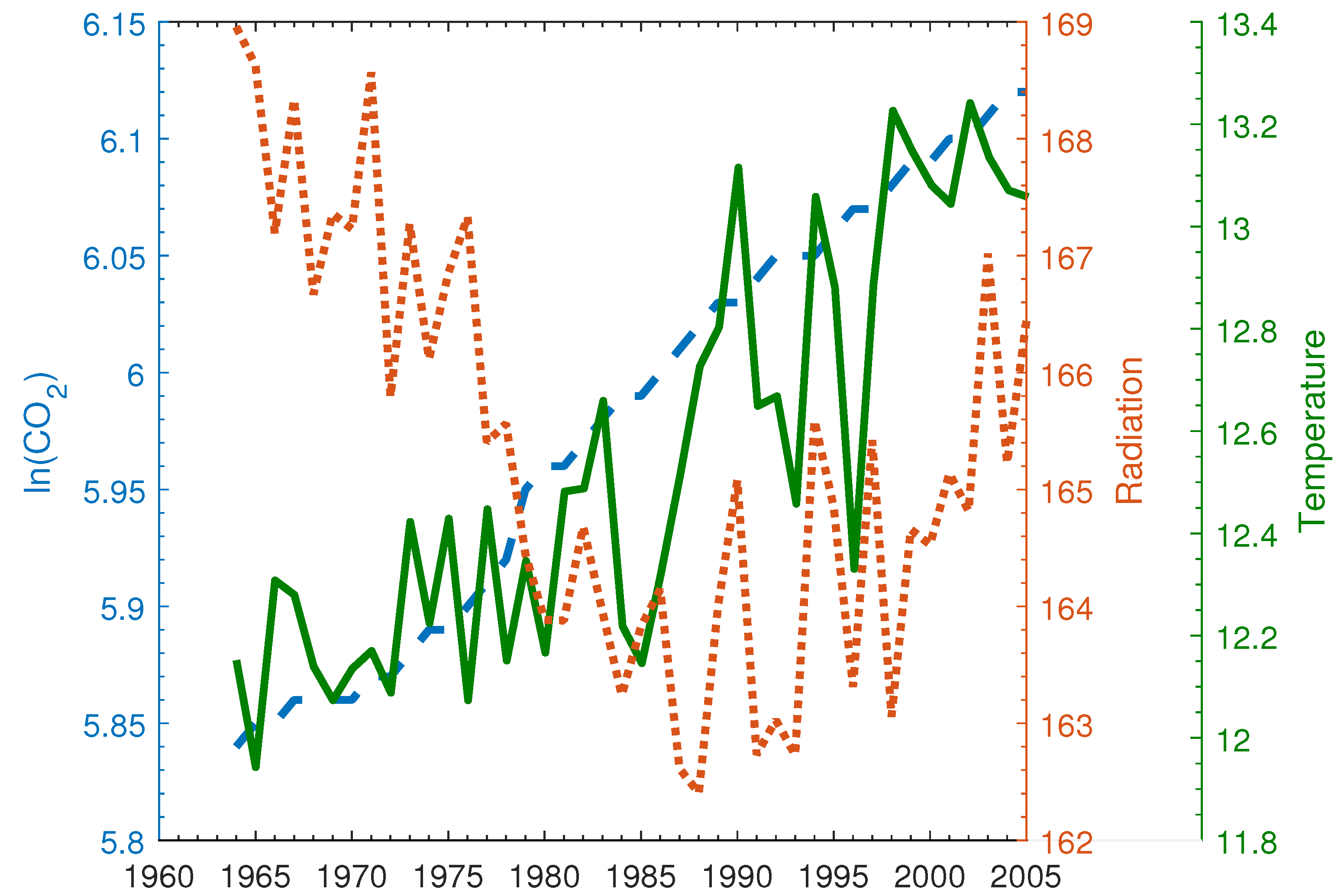
Equation (2) may be interpreted as a form of energy balance relationship that captures the global linkage between temperature, radiation and greenhouse gas atmospheric influences, allowing for the presence of stochastic and deterministic trend effects. The balance in these global elements is measured by ${\lambda }_t$ and is assumed to be one of the drivers impacting local temperature in the subsequent time period. The dynamic panel regression Equation (1) therefore characterizes the dynamic adjustment mechanism of station level temperature $T_{it+1}$ as an autoregression on past temperature $T_{it},$ radiation $R_{it},$ and global energy balancing effects ${\lambda }_t.$ Equation (2) is specified without error, so that the observed aggregate variables $\left(T_t,R_t,\ln \left(C{O}_{2,t}\right)\right)$ are assumed to impact station-level temperature in (1) directly without noise. The possibility of including unobserved noise in the specification of ${\lambda }_t$ and the impact on the asymptotic theory of this inclusion of measurement error in (2) is considered later in the paper. Phillips et al. (2020) provide a detailed discussion of the specification of (1)–(5) and the justification for these equations in terms of relevant atmospheric considerations and empirical assessments using observed data. The global variables are shown in Figure 1 over the time period 1964–2005.

The following Assumptions 1(i)–(vi) concern various components of the panel system (1)–(5). They are related to but stronger than the conditions used in Phillips et al. (2020). More specifically, the assumption of independent and identically distributed ($iid$) equation errors in Assumption 1(i), (iii) and (iv) and the assumption of independence of the errors across equations in Assumption 1(i) are useful and commonly employed to establish limit theory for panel regression estimation procedures such as WG, diff-GMM and sys-GMM for which endogenous regressors and equation error serial dependence typically produce bias and inconsistencies. These stronger conditions are not needed for the aggregate time series approach in Phillips et al. (2020) where estimation by FM-OLS cointegrating regression was used. Readers are referred to that work for a detailed discussion of the more relaxed conditions used with that methodology. Specific implications of the present assumptions on convergence rates and asymptotic bias and efficiency are discussed later in the paper.

Assumption 1.

(i) 

The panel regression errors $\left\{u_{it}\right\}{\sim }_{iid}\left(0,{\sigma }_u^2\right)$ over i and t and are independent of the random sequences $\left\{u_{it}^P\right\},\left\{{\delta }_{ri}\right\},\left\{u_{ct}\right\}$ for all $\left(i,t\right).$ The idiosyncratic loading factors $\left\{{\delta }_{ri}\right\}$ ${\sim }_{iid}\left({\delta }_r,{\Sigma }_r\right)$ and station-level effects ${\alpha }_i{\sim }_{iid}\left(\alpha ,{\sigma }_{\alpha }^2\right)$ are independent and both are independent of $\left\{u_{it}^P\right\},\left\{u_{ct}\right\}$ for all $\left(i,t\right),$ where the $\left\{u_{it}^P\right\}$ are defined in A(iii) and the $\left\{u_{ct}\right\}$ in A(iv).

(ii) 

${\overline{R}}_t^0=N^{-1}{\sum }_{i=1}^N{R}_{it}^0{\to }_{a.s.}{R}^0={\lim }_{N\to \infty }\left\{N^{-1}{\sum }_{i=1}^N\mathbb{E}\left(R_{it}^0\right)\right\}.$

(iii) 

$P_{it}=P_{i0}+{\sum }_{k=1}^t{u}_{ik}^P=:P_{i0}+U_{it}^P$ where $u_{ik}^P{\sim }_{iid}\left(0,{\sigma }_p^2\right)$ with finite fourth moments over i and t,

$${\overline{P}}_0=N^{-1}\sum _{i=1}^N{P}_{i0}{\to }_{a.s.}{P}^0=\underset{N\to \infty }{\lim }\left\{N^{-1}\sum _{i=1}^N\mathbb{E}\left(P_{it}^0\right)\right\},$$

$N^{-1/2}{\sum }_{i=1}^N\left(P_{i0}-\mathbb{E}\left(P_{it}^0\right)\right)=O_p\left(1\right)$ and the partial sums $U_{it}^P$ satisfy the invariance principle $n^{-1/2}{U}_{it}^P\Rightarrow U_i^P\left(r\right)\equiv BM\left({\sigma }_P^2\right)$ for all $i.$

(iv) 

$u_{gt}{\sim }_{iid}\left(0,{\Sigma }_g\right)$ with finite fourth moments has partial sums $U_{gt}={\sum }_{k=1}^t{u}_{gk}$ that satisfy the invariance principle $n^{-1/2}{U}_{g\lfloor nr\rfloor }\Rightarrow U_g\left(r\right)\equiv BM\left({\Sigma }_g\right),$ vector Brownian motion with covariance matrix ${\Sigma }_g>0;$ and $u_{ct}{\sim }_{iid}\left(0,{\sigma }_c^2\right)$ with finite fourth moments has partial sums $U_{ct}={\sum }_{k=1}^t{u}_{ck}$ which satisfy the invariance principle $n^{-1/2}{U}_{c\lfloor nr\rfloor }\Rightarrow U_c\left(r\right)\equiv BM\left({\sigma }_c^2\right),$ with ${\sigma }_c^2>0.$

(v) 

$\left|{\beta }_1\right|<1$, $\left|{\beta }_1+{\gamma }_1\right|<1.$

(vi) 

$\left(n,N\right)\to \infty$ with $\frac{n}{N}+\frac{N}{n^3}\to 0.$

An important feature of the model (1) and (2) is that it can be used to measure transient climate sensitivity (TCS) to $C{O}_2$ emissions. This parameter plays a major role in discussions about the potential impact of greenhouse gas emissions on Earth’s climate. TCS is defined as the expected global temperature after a doubling of $C{O}_2$ and has the following analytic form (Magnus et al. 2011; Storelvmo et al. 2016)

$$TCS=\frac{{\gamma }_3}{1-{\beta }_1-{\gamma }_1}\times \ln \left(2\right).$$

(6)

Phillips et al. (2020) developed a simple and direct cointegration regression approach to the estimation of the parameter $TCS$ using the long run relationship among the variables $\left(T_t,R_t,\ln \left(C{O}_{2,t}\right)\right)$ that is implied by (1) and (2). A different, station-level approach is to estimate the parameters of the dynamic panel regression model (1) combined with the parameters that appear in the aggregate balancing relation (2) and to use these estimates in conjunction with Formula (6) to obtain an estimate of $TCS$ and an associated confidence interval.

The present contribution is concerned primarily with studying this station-level approach to estimation. As expected, the limit theory of $TCS$ estimates obtained in this way from estimates of the complete model differ from those obtained by fitting the long-run relationship alone. Full panel regression estimation of the system (1) and (2) can be performed in various ways, for instance, by WG, diff-GMM, and sys-GMM techniques, with many additional variations depending on the precise selection of instrumental variables in the use of diff-GMM and sys-GMM techniques. Intriguingly, as we show in Theorem 1 below, the resulting estimates of (6) obtained in this way turn out to be invariant to the method employed in the panel regression estimation of (1) and (2). This invariance holds even though the individual parameter estimates of $\left({\beta }_1,{\beta }_2,{\gamma }_1,{\gamma }_2\right)$ obtained by WG, diff-GMM, and sys-GMM differ. In some cases, particularly sys-GMM, the differences are huge—see

Table 1. Dynamic panel regression and transient climate sensitivity estimates.

	Estimation Method
	WG	diff-GMM	sys-GMM
Parameter
${\beta }_1$	0.1346	0.1125	0.8665
${\beta }_2$	−0.0001	−0.0048	0.0098
${\gamma }_1$	−0.0230	−0.0010	−0.7549
${\gamma }_2$	0.0262	0.0309	0.0162
${\gamma }_3$	3.6400	3.6400	3.6400
${\beta }_1+{\gamma }_1$	0.1116	0.1116	0.1116
${\beta }_2+{\gamma }_2$	0.0261	0.0261	0.0260
$r_{\alpha }=\frac{{\sigma }_{\alpha }}{{\sigma }_u}$	15.043	12.825	1.4769
$TCS$	2.8399	2.8399	2.8399

Notes:$r_{\alpha }=\frac{{\sigma }_{\alpha }}{{\sigma }_u}={\left(\frac{\mathbb{V}\left({\alpha }_i\right)}{\mathbb{V}\left(u_{it}\right)}\right)}^{1/2}$.

below and the attendant discussion. These differences arise primarily because of the substantial heterogeneity in the fixed effects ${\alpha }_i$ in the climate panel regression Equation (1), which capture the large local variation in station temperature levels.

3. Estimation by Dynamic Panel Regression

3.1. Common Trends and Global Cointegration

The system (1) and (2) involves the station-level panel adjustment mechanism (1) with global effects imparted by the time specific effects ${\lambda }_t,$ which in turn depend on global averages over stations. To reconcile these two components, aggregation of (1) gives

$$T_{t+1}=\overline{\alpha }+{\beta }_1{T}_t+{\beta }_2{R}_t+{\lambda }_t+\frac{1}{N}\sum _{i=1}^N{u}_{it+1}=\overline{\alpha }+{\beta }_1{T}_t+{\beta }_2{R}_t+{\lambda }_t+{\overline{u}}_{·t+1},$$

where $\overline{\alpha }=N^{-1}{\sum }_{i=1}^N{\alpha }_i$ and ${\overline{u}}_{·t+1}=N^{-1}{\sum }_{i=1}^N{u}_{it+1}.$ Following standard practice for identification purposes in the presence of fixed individual and time effects, we set $\overline{\alpha }=0.$ Substituting (2) gives the global equation

$$T_{t+1}={\gamma }_0+\left({\beta }_1+{\gamma }_1\right)T_t+\left({\beta }_2+{\gamma }_2\right)R_t+{\gamma }_3\ln \left(C{O}_{2,t}\right)+{\overline{u}}_{·t+1}.$$

(7)

Setting ${\theta }_1={\beta }_1+{\gamma }_1$ and ${\theta }_2={\beta }_2+{\gamma }_2,$ it is convenient to write (7) as

$$T_{t+1}={\gamma }_0+{\theta }_1{T}_t+{\theta }_2{R}_t+{\gamma }_3\ln \left(C{O}_{2,t}\right)+{\overline{u}}_{·t+1},$$

(8)

and solving by back substitution gives the stochastic trend representation of $T_t,$ in conjunction that of with $\left(R_t,\ln \left(C{O}_{2,t}\right)\right),$ which is given in Phillips et al. (2020, Theorem 1), viz.,

$$W_t=\left[\begin{array}{c}{T}_t\\ R_t\\ \ln \left(C{O}_{2,t}\right)\end{array}\right]=\left[\begin{array}{c}{\delta }_{T0}+{\delta }_{T1}t+{\delta }_T^{\prime }{U}_{gt}+u_{Tt}^{+}\\ {\delta }_{r0}+{\delta }_r^{\prime }{U}_{gt}+O_p\left(\sqrt{\frac{n}{N}}\right)\\ {\delta }_{c0}+{\delta }_{c1}t+{\delta }_c^{\prime }{U}_{gt}+u_{ct}\end{array}\right]=:{\delta }_{w0}+{\delta }_{w1}t+D_w{U}_{gt}+u_{wt}^{+},$$

(9)

where

$$\begin{array}{ccc}\hfill {\delta }_{T1}& =& \frac{{\gamma }_3{\delta }_{c1}}{1-{\theta }_1},{\delta }_T=\frac{{\theta }_2{\delta }_r+{\gamma }_3{\delta }_c}{1-{\theta }_1},\hfill \end{array}$$

(10)

$$\begin{array}{ccc}\hfill u_{Tt}& =& {\gamma }_3\sum _{j=0}^{\infty }{\theta }_1^j{u}_{ct-1-j}-\frac{{\theta }_1}{1-{\theta }_1}\sum _{k=0}^{\infty }{\theta }_1^k{\left[{\theta }_2{\delta }_r+{\gamma }_3{\delta }_c\right]}^{\prime }{u}_{gt-1-k}-{\delta }_T^{\prime }{u}_{gt},\hfill \end{array}$$

(11)

$$\begin{array}{ccc}\hfill u_{Tt}^{+}& =& u_{Tt}+O_p\left(\frac{1}{\sqrt{N}}+\sqrt{\frac{n}{N}}+t{\left|{\theta }_1\right|}^t\right),\hfill \end{array}$$

(12)

where $D_w^{\prime }=\left[{\delta }_T,{\delta }_r,{\delta }_c\right],$ ${\delta }_{w0}={\left[{\delta }_{T0},{\delta }_{r0},{\delta }_{c0}\right]}^{\prime },{\delta }_{w1}={\left[{\delta }_{T1},0,{\delta }_{c1}\right]}^{\prime },u_{wt}^{+}=u_{wt}+O_p\left(\frac{1}{\sqrt{N}}+\sqrt{\frac{n}{N}}+t{\left|{\theta }_1\right|}^t\right)$ and $u_{wt}={\left[u_{Tt},0,u_{ct}\right]}^{\prime }.$

From the trend representation (9), the following long run cointegrating relationship among the global variables $\left(T_t,R_t,\ln \left(C{O}_{2,t}\right)\right)$ is obtained

$$T_t=\frac{{\theta }_2}{1-{\theta }_1}{R}_t+\frac{{\gamma }_3}{1-{\theta }_1}\ln \left(C{O}_{2,t}\right)+\frac{\mu }{1-{\theta }_1}+\frac{1}{1-{\theta }_1}{\zeta }_t,$$

(13)

using: (i) the fact that ${\delta }_T=\frac{{\theta }_2{\delta }_r+{\gamma }_3{\delta }_c}{1-{\theta }_1},$ which delivers cointegration among the stochastic trend components of $\left(T_t,R_t,\ln \left(C{O}_{2,t}\right)\right)$; and (ii) the linkage ${\delta }_{T1}=\frac{{\gamma }_3{\delta }_{c1}}{1-{\theta }_1},$ which ensures deterministic co-movement of the linear trends in $T_t$ and $\ln \left(C{O}_{2,t}\right).$ The equation error (or equilibrium error correction) in (13) is

$$\frac{1}{1-{\theta }_1}{\zeta }_t=u_{Tt}-\frac{{\gamma }_3}{1-{\theta }_1}{u}_{ct}+O_p\left(\frac{1}{\sqrt{N}}+\sqrt{\frac{n}{N}}+t{\left|{\theta }_1\right|}^t\right),$$

(14)

which is a stationary, weakly dependent time series up to an asymptotically negligible component.

Importantly, the cointegrating relation (13) is distinct from the time specific effect ${\lambda }_t.$ In fact, (13) represents the ultimate global linkage in these variables that results from integrating the time specific effects ${\lambda }_t$ with the station-level adjustment mechanism and the global aggregation process that leads to $\left(T_t,R_t,\ln \left(C{O}_{2,t}\right)\right).$ Moreover, the coefficient of $\ln \left(C{O}_{2,t}\right)$ in the relationship (13) gives the transient climate sensitivity parameter (6) upon scaling by $\ln \left(2\right)$

$$TCS=\frac{{\gamma }_3}{1-{\theta }_1}\times \ln \left(2\right)=\frac{{\gamma }_3}{1-{\beta }_1-{\gamma }_1}\times \ln \left(2\right),$$

(15)

which means that the $TCS$ parameter can be estimated directly from appropriate econometric estimation (such as fully-modified least squares (FM-OLS)) of the long run cointegrating relation (13) without regard to the dynamic adjustment mechanism (1). That approach was followed in Phillips et al. (2020) where an asymptotic theory of inference was developed for the methodology. The present work instead pursues a panel regression approach although we do discuss later a key difference between the asymptotic theory of the resulting FM-OLS of $TCS$ and the asymptotic theory of estimates of $TCS$ based on panel regression estimates such as WG, diff-GMM, and sys-GMM.

3.2. Dynamic Panel Estimation and Invariance Properties

The alternative station-level approach uses panel regression methods to estimate both (1) and (2). This approach was used in Magnus et al. (2011) and Storelvmo et al. (2016). Specifically, sys-GMM methods were employed by Magnus et al. (2011) and Storelvmo et al. (2016) because their estimates of the panel autoregressive coefficient ${\beta }_1$ exceeded $0.9$ and dynamic panel regressions with autoregressive coefficients close to unity are known to lead to weak instrumentation in diff-GMM methods, thereby reducing efficiency but retaining consistency (Kruiniger 2009; Phillips 2018). In the present application, as might be expected given the global coverage of the station-level observations, there is considerable heterogeneity in the fixed effects ${\alpha }_i$ of the dynamic panel regression (1), a feature that is known to produce sys-GMM estimates of the coefficients in dynamic panel regression that can be substantially biased (Hayakawa 2007, 2015). For this reason, we might expect some large differences in the coefficient estimates among these three panel regression procedures.

For the observational data used in Storelvmo et al. (2016) and Phillips et al. (2020), the differences are substantial, particularly between sys-GMM and the other two approaches. Table 1 below provides estimates of the parameters of the system defined in (1) and (2). The massive difference between the sys-GMM estimate of the parameter ${\beta }_1$ ($0.8665)$ and the estimates obtained by diff-GMM ($0.1125$) and WG ($0.1346$) is striking—the sys-GMM estimate is more than six times greater than the WG estimate and nearly eight times greater than the diff-GMM estimate. The implications of these differences for the station-level dynamic adjustment mechanism of temperature are enormous. Similar major differences occur in the estimation of the parameter ${\gamma }_1$ in the aggregate relation for ${\lambda }_t.$ Table 1 also reports the ratio $r_{\alpha }={\widehat{\sigma }}_{\alpha }/{\widehat{\sigma }}_u$ of the estimated standard deviation ${\widehat{\sigma }}_{\alpha }$ of the fitted fixed effects ${\alpha }_i$ to the standard deviation of the fitted equation errors $u_{i,t+1}.$ For the WG estimates, this ratio is 15.043, which is ten times greater than the corresponding value from sys-GMM, showing the major differences in how the two methods capture and represent the observed variation in the data at the local level.

Even more striking is that, in spite of the differences in the estimates of the individual coefficients, estimates of the composite parameters ${\beta }_1+{\gamma }_1,$ ${\beta }_2+{\gamma }_2,$ and the transient climate sensitivity parameter $TCS$ are all invariant to the method of estimation of the dynamic panel regression equation. This equivalence is established analytically in Theorem 1 below. An important implication of this analytic invariance is that the $TCS$ estimate has the same asymptotic theory for the different panel regression methods and thus the same induced asymptotic confidence interval.

To proceed, it is convenient to write the model (1) and (2) in the form:

$$\begin{array}{ccc}\hfill T_{i,t+1}& =& {\alpha }_i+{\beta }_1{T}_{i,t}+{\beta }_2{R}_{i,t}+{\lambda }_t+u_{it+1}=:{\alpha }_i+{\beta }^{\prime }{X}_{it}+{\lambda }_t+u_{it+1}\hfill \end{array}$$

(16)

$$\begin{array}{ccc}\hfill {\lambda }_t& =& {\gamma }_0+{\gamma }_1{T}_t+{\gamma }_2{R}_t+{\gamma }_3\ln \left(C{O}_{2,t}\right)=:{\gamma }_0+{\gamma }^{\prime }{W}_t,\hfill \end{array}$$

(17)

with notation $X_{it}={\left(T_{i,t},R_{i,t}\right)}^{\prime }$ and $W_t={\left(T_t,R_t,\ln \left(C{O}_{2,t}\right)\right)}^{\prime }.$ It follows by aggregation and the normalization condition $\overline{\alpha }=0$ that

$$T_{t+1}={\beta }^{\prime }{X}_t+{\lambda }_t+{\overline{u}}_{·t+1}=\left({\beta }^{\prime },0\right)W_t+{\lambda }_t+{\overline{u}}_{·t+1}.$$

The model (16) and (17) can also be written in the combined factor augmented form

$$T_{i,t+1}={\gamma }_0+{\alpha }_i+{\beta }^{\prime }{X}_{i,t}+{\gamma }^{\prime }{W}_t+u_{it+1},$$

(18)

which is a dynamic panel model with a common factor given by the component ${\gamma }^{\prime }{W}_t$ with observable $W_t.$ The technical complications involved in the analysis of (18) arise because: (i) the common factor aggregate $W_t={\left({\overline{X}}_{·t}^{\prime },\ln \left(C{O}_{2,t}\right)\right)}^{\prime }$ relates to the observable station level variables $X_{it}$ that appear as regressors in (18), as well as the exogenous variable $C{O}_{2,t};$ (ii) the regressors $\left(X_{i,t},W_t\right)$ have deterministic and stochastic trend components; and (iii) there is cointegration (both deterministic and stochastic) among the elements of the global aggregate $W_t.$ Aggregating (18) and using the identification condition $\overline{\alpha }=0$ gives (8). Setting

$$\theta ={\left({\theta }_1,{\theta }_2,{\theta }_3\right)}^{\prime }={\left({\beta }_1+{\gamma }_1,{\beta }_2+{\gamma }_2,{\gamma }_3\right)}^{\prime },$$

the global dynamic regression is

$$T_{t+1}={\gamma }_0+{\theta }_1{T}_t+{\theta }_2{R}_t+{\gamma }_3\ln \left(C{O}_{2t}\right)+{\overline{u}}_{·t+1}={\gamma }_0+{\theta }^{\prime }{W}_t+{\overline{u}}_{·t+1},$$

(19)

which it is convenient to write in observation form as

$$T^{+}={\gamma }_0{\iota }_{n-1}+W\theta +{\overline{U}}^{+}={\left(T_2,T_3,\dots ,T_n\right)}^{\prime }$$

(20)

where $T^{+}={\left(T_2,T_3,\dots ,T_n\right)}^{\prime },$ ${\overline{U}}^{+}={\left[{\overline{u}}_{·2},\dots ,{\overline{u}}_{·n}\right]}^{\prime },$ and ${\iota }_{n-1}$ is an $\left(n-1\right)$ vector of ones.

We now proceed to analyze the estimation of this station-level system and to develop asymptotic theory for the resulting coefficient estimates and the associated TCS parameter. For the purpose of the discussion below it is convenient to work with the WG estimator. However, as will be demonstrated, the results obtained for the $TCS$ parameter estimates (and for certain linear contrasts of the other coefficients, notably ${\beta }_1+{\gamma }_1$ and ${\beta }_2+{\gamma }_2$) apply also to diff-GMM and sys-GMM procedures.

The WG procedure involves the following steps.

Step 1.

Estimate the dynamic panel model by least squares, which involves estimating the time specific effect ${\lambda }_t$ as the time specific intercept in the regression (1). That is, applying least squares with intercept standardized so that $\overline{\alpha }=0,$ we obtain

$${\widehat{\lambda }}_t=T_{t+1}-{\widehat{\beta }}^{\prime }{X}_t=T_{t+1}-{\widehat{\beta }}_1{T}_t-{\widehat{\beta }}_2{R}_t=T_{t+1}-\left({\widehat{\beta }}^{\prime },0\right)W_t,$$

(21)

with

$$\widehat{\beta }={\left(\sum _{t=1}^{n-1}\sum _{i=1}^N{\tilde{X}}_{i,t}{\tilde{X}}_{i,t}^{\prime }\right)}^{-1}\left(\sum _{t=1}^{n-1}\sum _{i=1}^N{\tilde{X}}_{i,t}{\tilde{T}}_{i,t+1}\right),$$

(22)

where we use the notation ${\tilde{A}}_{it}=A_{it}-{\overline{A}}_{i·}-{\overline{A}}_t.+{\overline{A}}_{··}$ with ${\overline{A}}_{i·}={\left(n-1\right)}^{-1}{\sum }_{t=1}^{n-1}{A}_{it},$ ${\overline{A}}_t.=N^{-1}{\sum }_{i=1}^N{A}_{it},$ and ${\overline{A}}_{··}={\left(n-1\right)}^{-1}{N}^{-1}{\sum }_{t=1}^{n-1}{\sum }_{i=1}^N{A}_{it}$. This means that the time specific and station specific effects are estimated by regression elimination and the slope coefficients $\beta$ are estimated using pooled least squares regression after elimination of these effects.

Step 2.

Regress the fitted ${\widehat{\lambda }}_t$ on $\left(1,T_t,R_t,\ln \left(C{O}_{2,t}\right)\right)$ by least squares giving

$${\widehat{\lambda }}_t={\widehat{\gamma }}_0+{\widehat{\gamma }}_1{T}_t+{\widehat{\gamma }}_2{R}_t+{\widehat{\gamma }}_3\ln \left(C{O}_{2,t}\right)={\widehat{\gamma }}_0+{\widehat{\gamma }}^{\prime }{W}_t,$$

(23)

and the corresponding vector of coefficient estimates $\left({\widehat{\gamma }}_0,{\widehat{\gamma }}^{\prime }\right)=\left({\widehat{\gamma }}_0,{\widehat{\gamma }}_1,{\widehat{\gamma }}_2,{\widehat{\gamma }}_3\right).$

Step 3.

Estimate the $TCS$ parameter using the coefficient estimates $\left({\widehat{\beta }}_1,{\widehat{\gamma }}_1,{\widehat{\gamma }}_3\right)$ giving

$$\widehat{TCS}=\frac{{\widehat{\gamma }}_3}{1-{\widehat{\beta }}_1-{\widehat{\gamma }}_1}\times \ln \left(2\right).$$

(24)

Steps 1 and 2 may be amalgamated in a combined least squares regression that minimizes the following objective function with respect to $\left({\alpha }_i,{\beta }^{\prime },{\gamma }_0,{\gamma }^{\prime }\right)$ subject to the identification condition that $\overline{\alpha }={\sum }_{i=1}^N{\alpha }_i=0$

$$\sum _{t=1}^{n-1}\sum _{i=1}^N{\left\{T_{i,t+1}-{\alpha }_i-{\beta }^{\prime }{X}_{i,t}-{\gamma }_0-{\gamma }^{\prime }{W}_t\right\}}^2,$$

(25)

which leads to the same estimates of the coefficients $\left(\widehat{\beta },\widehat{\gamma }\right)$ as those obtained by following Steps 1 and 2 above. Writing the vector of estimated time effects obtained in Step 1 as $\widehat{\lambda }=\left({\widehat{\lambda }}_t\right),$ it is apparent from (23) that the slope coefficient estimates of $\gamma$ in the regression (23) take the form

$$\widehat{\gamma }={\left({\tilde{W}}^{\prime }\tilde{W}\right)}^{-1}\left({\tilde{W}}^{\prime }\widehat{\lambda }\right).$$

(26)

where $\tilde{W}=W-\overline{W}$ is the matrix of deviations from time series means ${\tilde{W}}_t=W_t-\overline{W}$.

The estimates $\left(\widehat{\beta },\widehat{\gamma }\right)$ and implied estimate $\widehat{TCS}$ of the $TCS$ parameter above are all obtained using WG estimation of the panel regression system (16) and (17). Somewhat remarkably, as the following result shows, the resulting estimate $\widehat{TCS}$ as well as the corresponding estimates of the linear contrasts ${\widehat{\theta }}_i={\widehat{\beta }}_i+{\widehat{\gamma }}_i,$ $\left(i=1,2\right),$ are invariant to the method of estimation of the panel regression equation estimates $\left(\widehat{\beta },\widehat{\gamma }\right),$ whether by WG, diff-GMM or sys-GMM.

Theorem 1.

Station-level estimation of the dynamic panel regression model (16) and (17) by the methods WG, diff-GMM, and sys-GMM all lead to the same common estimate $\widehat{\theta }={\left({\tilde{W}}^{\prime }\tilde{W}\right)}^{-1}{\tilde{W}}^{\prime }{T}^{+}$ of the slope coefficient θ in (19) and the common estimate of the $TCS$ parameter

$$\widehat{TCS}=\frac{{\widehat{\gamma }}_3}{1-{\widehat{\theta }}_1}\times \ln \left(2\right).$$

Remark 1.

Given the substantial differences among the methods WG, diff-GMM and sys-GMM, it may seem remarkable that the composite estimates $\left({\widehat{\beta }}_1+{\widehat{\gamma }}_1\right)$ and $\left({\widehat{\beta }}_2+{\widehat{\gamma }}_2\right)$ are invariant to the panel regression method employed. The individual estimates $\left({\widehat{\beta }}_1,{\widehat{\beta }}_2,{\widehat{\gamma }}_1,{\widehat{\gamma }}_2\right)$ obtained by the methods WG, diff-GMM and sys-GMM are not invariant but the estimated coefficients ${\widehat{\beta }}_i$ and ${\widehat{\gamma }}_i$ involve compensatory adjustments that ensure invariance of the contrasts $\left({\widehat{\beta }}_1+{\widehat{\gamma }}_1\right)$ and $\left({\widehat{\beta }}_2+{\widehat{\gamma }}_2\right).$ As shown in the proof of Theorem 1 these adjustments ensure that the estimation error for the composite estimate $\widehat{\theta }$ of θ in (20) satisfy the system

$$\widehat{\theta }-\theta ={\left({\tilde{W}}^{\prime }\tilde{W}\right)}^{-1}{\tilde{W}}^{\prime }{T}^{+}-\theta =\left[\begin{array}{c}\left({\widehat{\beta }}_1+{\widehat{\gamma }}_1\right)-\left({\beta }_1+{\gamma }_1\right)\\ \left({\widehat{\beta }}_2+{\widehat{\gamma }}_2\right)-\left({\beta }_2+{\gamma }_2\right)\\ \left({\widehat{\gamma }}_3-{\gamma }_3\right)\end{array}\right],$$

(27)

which is determined solely by least squares regression of (the aggregate time series matrices) $T^{+}$ on $\tilde{W},$ making the estimation error $\widehat{\theta }-\theta$ of the composite parameters invariant to the method of estimation of the panel regression Equation (16).

Remark 2.

The intuitive explanation for this invariance is that the individual estimated coefficients ${\widehat{\beta }}_i$ in (16) depend on data $\left(T_{i,t+1},X_{i,t}\right)$ that upon aggregation necessarily satisfy the global dynamic relationship (19), which upon time series demeaning is just ${\tilde{T}}_{t+1}={\theta }^{\prime }{\tilde{W}}_t+{\tilde{\overline{u}}}_{·t+1},$ where ${\tilde{T}}_{t+1}=T_{t+1}-\overline{T}$ and ${\tilde{W}}_t=W_t-\overline{W}.$ The temporally demeaned linear time series relationship ${\tilde{T}}_{t+1}={\theta }^{\prime }{\tilde{W}}_t+{\tilde{\overline{u}}}_{·t+1}$ involves only the composite vector θ in its systematic part. Thus, the parameter θ may be interpreted as a global composite parameter and this aggregate relationship may be interpreted as a reduced form dynamic equation for the global variables. The estimates $\left({\widehat{\beta }}_1,{\widehat{\beta }}_2\right)$ of the system parameters $\left({\beta }_1,{\beta }_2\right)$ are used to estimate the time specific effects ${\lambda }_t$ by cross section aggregation giving ${\widehat{\lambda }}_t$ as shown in (21) with ${\widehat{\lambda }}_t=T_{t+1}-\left({\widehat{\beta }}^{\prime },0\right)W_t$. Correspondingly, when the parameter γ is estimated in (23) using these specific fitted values ${\widehat{\lambda }}_t,$ we have $\widehat{\gamma }={\left({\tilde{W}}^{\prime }\tilde{W}\right)}^{-1}\left({\tilde{W}}^{\prime }\widehat{\lambda }\right)$, so that the resulting estimates satisfy

$$\widehat{\gamma }={\left({\tilde{W}}^{\prime }\tilde{W}\right)}^{-1}{\tilde{W}}^{\prime }\left\{T^{+}-W\left[\begin{array}{c}\widehat{\beta }\\ 0\end{array}\right]\right\}={\left({\tilde{W}}^{\prime }\tilde{W}\right)}^{-1}{\tilde{W}}^{\prime }{T}^{+}-\left[\begin{array}{c}\widehat{\beta }\\ 0\end{array}\right]$$

(28)

and transposition gives

$$\widehat{\theta }={\left({\tilde{W}}^{\prime }\tilde{W}\right)}^{-1}\left({\tilde{W}}^{\prime }{T}^{+}\right)=\left[\begin{array}{c}{\widehat{\beta }}_1+{\widehat{\gamma }}_1\\ {\widehat{\beta }}_2+{\widehat{\gamma }}_2\\ {\widehat{\gamma }}_3\end{array}\right],$$

(29)

showing invariance and the manner in which the compensatory adjustments in the composite estimates are automatically embodied by virtue of the cross section aggregation and the regression (23). In effect, the estimate $\widehat{\gamma }$ adjusts to whichever specific fitted values ${\widehat{\lambda }}_t$ are obtained from the particular panel regression method of estimation that produces the estimates $\left({\widehat{\beta }}_1,{\widehat{\beta }}_2\right).$ Thus, the estimates $\left({\widehat{\beta }}_1+{\widehat{\gamma }}_1\right),$ $\left({\widehat{\beta }}_2+{\widehat{\gamma }}_2\right),$ and ${\widehat{\gamma }}_3$ of $\left({\beta }_1+{\gamma }_1\right),$ $\left({\beta }_2+{\gamma }_2\right),$ and ${\gamma }_3$ are each invariant to the choice of estimation procedure for the coefficients β in the panel regression (16). In every case, the estimate $\widehat{\theta }$ of the composite parameter θ ends up taking the same value and is invariant to the panel regression method.

4. Asymptotic Theory

In view of the invariance properties established in Theorem 1, it is convenient to do the analysis with the (invariant) composite parameter estimate $\widehat{\theta }$ and the implied estimate $\widehat{TCS}.$ It is also convenient to fix ideas by working with the WG estimates of the parameters $\left(\beta ,\gamma \right)$ and, hence, $\theta$ and $TCS.$

We start by writing the common trend representation (9) as

$$W_t={\delta }_{w0}+{\delta }_{w}t+V_t+u_{wt}^{+},$$

(30)

where $V_t=D_w{U}_{gt}=:{\left[V_{Tt},V_{rt},V_{ct}\right]}^{\prime },$ and ${\delta }_w={\left({\delta }_{T1},0,{\delta }_{c1}\right)}^{\prime }.$ Subtracting time series means gives ${\tilde{W}}_t={\delta }_w\tilde{t}+{\tilde{V}}_t+{\tilde{u}}_{wt}^{+},$ with ${\tilde{V}}_t=V_t-\overline{V}.$ Then

$$\widehat{\theta }-\theta ={\left({\tilde{W}}^{\prime }\tilde{W}\right)}^{-1}\left({\tilde{W}}^{\prime }{\overline{U}}^{+}\right),$$

(31)

and the limit theory needs to take account of degeneracy in the asymptotic form of the sample moment matrix ${\tilde{W}}^{\prime }\tilde{W}={\sum }_{t=1}^n{\tilde{W}}_t{\tilde{W}}_t^{\prime }$ arising from the presence of both linear and stochastic trends in $W_t.$ We remark also that asymptotics for the second component of (31), ${\tilde{W}}^{\prime }{\overline{U}}^{+}={\sum }_{t=1}^n{\tilde{W}}_t{\overline{u}}_{·t+1},$ depends on the behavior of the cross section averaged elements ${\overline{u}}_{·t+1}=$ $N^{-1}{\sum }_{i=1}^N{u}_{i,t+1}.$ Under Assumption 1(i) and using ⇝ to denote weak convergence, these elements satisfy a CLT $\sqrt{N}{\overline{u}}_{·t+1}⇝{\xi }_{t+1},$ say, and are therefore of order $O_p\left(N^{-1/2}\right).$ Further, in view of Assumptions 1(i)–(iv), we have the functional laws $n^{-1/2}{V}_{\lfloor nr\rfloor }⇝V\left(r\right),$ $n^{-1/2}{\tilde{V}}_{\lfloor nr\rfloor }⇝\tilde{V}\left(r\right)=V\left(r\right)-{\int }_0^{1}V\left(s\right)ds,$ and an implied functional law for partial sums of the limit variates ${\xi }_{t+1},$ viz., $n^{-1/2}{\sum }_{t=1}^{\lfloor nr\rfloor }{\xi }_t⇝B_{\xi }\left(r\right)\equiv BM\left({\sigma }_{\xi }^2\right),$ where ${\sigma }_{\xi }^2=\mathbb{E}\left({\xi }_t^2\right)={\sigma }_u^2.$

To handle the asymptotic degeneracy of the sample moment matrix, we proceed in the usual fashion by rotation of the coordinate system of the regressors to isolate directions of different magnitudes (Park and Phillips 1988, 1989). Define the deterministic trend direction $h={\delta }_w/{\left({\delta }_w^{\prime }{\delta }_w\right)}^{1/2}$ in (30) and let $H_{\perp }$ be an orthogonal complement of h so that the matrix

$$H=[h,H_{\perp }]=\frac{1}{{\left({\delta }_w^{\prime }{\delta }_w\right)}^{1/2}}\left[\begin{array}{ccc}\frac{{\delta }_{c1}{\gamma }_3}{1-{\theta }_1}& 0& -{\delta }_{c1}\\ 0& {\left({\delta }_w^{\prime }{\delta }_w\right)}^{1/2}& 0\\ {\delta }_{c1}& 0& \frac{{\delta }_{c1}{\gamma }_3}{1-{\theta }_1}\end{array}\right],$$

(32)

is orthogonal and ${\delta }_w^{\prime }{\delta }_w={\left(\frac{{\delta }_{c1}}{1-{\theta }_1}\right)}^2\left\{{\left(1-{\theta }_1\right)}^2+{\gamma }_3^2\right\}.$ Rotating the system by H gives

$$H^{\prime }{\tilde{W}}_t=\left\{\begin{array}{c}a\tilde{t}+h^{\prime }{\tilde{V}}_t+O_p\left(1\right)\\ V_{\perp t}+O_p\left(1\right)\end{array}\right.,\mathrm{with}a={\left({\delta }_w^{\prime }{\delta }_w\right)}^{1/2},$$

(33)

which isolates the deterministic trend in the leading coordinate and the stochastic trend in the remaining coordinates, which we have written as $V_{\perp t}=H_{\perp }^{\prime }{V}_t$. Corresponding to these coordinates, define the scaling matrix $D_n=\mathrm{diag}\left(n^{3/2},n{I}_2\right).$

With these preliminaries, we are able to state the following asymptotic result concerning the composite parameter estimate $\widehat{\theta }$ in (31) and its mixed normal ($\mathcal{MN}$) limit theory corresponding to the different directions of deterministic and stochastic trends in the component variables. The presence of mixed normality may appear unusual in panel regression setting where sequential cross section and time series asymptotics commonly lead to standard normal limit theory. In the present case, the key parameters (including the $TCS$ parameter) rely on the coefficient of ${\lambda }_t$ in what is effectively an aggregate time series regression among global variables that have deterministically and stochastically nonstationary characteristics. Thus, in (26) we have $\widehat{\gamma }={\left({\tilde{W}}^{\prime }\tilde{W}\right)}^{-1}\left({\tilde{W}}^{\prime }\widehat{\lambda }\right)$ and in (29) $\widehat{\theta }={\left({\tilde{W}}^{\prime }\tilde{W}\right)}^{-1}\left({\tilde{W}}^{\prime }{T}^{+}\right),$ both involving the nonstationary components of $\tilde{W}.$ These features of the regression leading to the estimate $\widehat{\theta }$ produce mixed normal limit theory in the same way that they do for conventional cointegrating regressions among nonstationary variables. Additional complications arise in the present case because the signal matrix ${\tilde{W}}^{\prime }\tilde{W}$ in this regression is asymptotically degenerate due to the presence of nonstationary components of different orders of magnitude. These complications are discussed in the remarks following Theorem 2.

In addition to $\widehat{\theta }$, Theorem 2 provides limit theory for the estimate of $TCS=\frac{{\theta }_3}{1-{\theta }_1}\times \ln \left(2\right)=:g\left({\theta }_a\right),$ where ${\theta }_a=\left({\theta }_1,{\theta }_3\right),$ based on the panel regression estimate ${\widehat{\theta }}_a.$

Theorem 2.

Under Assumption 1 and as $\left(n,N\right)\to \infty :$

(i) 

$n\sqrt{N}\left(\widehat{\theta }-\theta \right)⇝H_{\perp }{\left({\int }_0^1{\tilde{V}}_{\perp ,\tilde{r}}{\tilde{V}}_{\perp ,\tilde{r}}^{\prime }\right)}^{-1}{\int }_0^1{\tilde{V}}_{\perp ,\tilde{r}}d{B}_{\xi }\equiv \mathcal{MN}\left(0,{\sigma }_{\xi }^2{H}_{\perp }{\left({\int }_0^1{\tilde{V}}_{\perp ,\tilde{r}}{\tilde{V}}_{\perp ,\tilde{r}}^{\prime }\right)}^{-1}{H}_{\perp }^{\prime }\right);$

(ii) 

$n^{3/2}\sqrt{N}{h}^{\prime }\left(\widehat{\theta }-\theta \right)⇝{\left(a{\int }_0^1{\tilde{r}}_{{\tilde{V}}_{\perp }}^2\right)}^{-1}\left({\int }_0^1{\tilde{r}}_{{\tilde{V}}_{\perp }}d{B}_{\xi }\right)\equiv \mathcal{MN}\left(0,\frac{{\sigma }_{\xi }^2}{a^2}{\left({\int }_0^1{\tilde{r}}_{{\tilde{V}}_{\perp }}^2\right)}^{-1}\right);$

(iii) 

$n^{3/2}\sqrt{N}\left(\widehat{TCS}-TCS\right)⇝\frac{1}{{\delta }_{c1}\left(1-{\theta }_1\right)}\frac{{\int }_0^1{\tilde{r}}_{{\tilde{V}}_{\perp }}d{B}_{\xi }}{{\int }_0^1{\tilde{r}}_{{\tilde{V}}_{\perp }}^2}\equiv \mathcal{MN}\left(0,\frac{{\sigma }_{\xi }^2}{{\delta }_{c1}^2{\left(1-{\theta }_1\right)}^2}{\left({\int }_0^1{\tilde{r}}_{{\tilde{V}}_{\perp }}^2\right)}^{-1}\right);$

where $\tilde{r}\left(r\right)=r-{\int }_0^{1}sds,$ ${\tilde{r}}_{{\tilde{V}}_{\perp }}=\tilde{r}-\left({\int }_0^1\tilde{r}{\tilde{V}}_{\perp }\right){\left({\int }_0^1{\tilde{V}}_{\perp }{\tilde{V}}_{\perp }^{\prime }\right)}^{-1}{\tilde{V}}_{\perp },$ $\tilde{V}\left(r\right)=V\left(r\right)-{\int }_0^{1}V\left(s\right)ds,$ and ${\tilde{V}}_{\perp ,r}\left(r\right)={\tilde{V}}_{\perp }\left(r\right)-\left({\int }_0^1{\tilde{V}}_{\perp }\tilde{r}\right){\left({\int }_0^1{\tilde{r}}^2\right)}^{-1}\tilde{r},$ ${\tilde{V}}_{\perp }\left(r\right)=H_{\perp }^{\prime }\tilde{V}\left(r\right)$.

Remark 3.

In (i) and (ii), ${\tilde{V}}_{\perp ,\tilde{r}}\left(r\right)$ is the $L_2$ projection residual of ${\tilde{V}}_{\perp }=H_{\perp }^{\prime }\tilde{V}$ on $\tilde{r},$ and ${\tilde{r}}_{{\tilde{V}}_{\perp }}$ is the $L_2$ projection residual of $\tilde{r}$ on ${\tilde{V}}_{\perp }.$ These projections are simply the equivalent in the limit theory of the projections that take place in finite samples. As is now familiar in nonstationary regression, transformations that occur in finite samples in Euclidean space are commonly reflected in the limit theory by projections in the corresponding $L_2$ space where the limiting stochastic processes lie, such as the projection residuals ${\tilde{V}}_{\perp ,r}\left(r\right)={\tilde{V}}_{\perp }\left(r\right)-\left({\int }_0^1{\tilde{V}}_{\perp }\tilde{r}\right){\left({\int }_0^1{\tilde{r}}^2\right)}^{-1}\tilde{r}$ and ${\tilde{r}}_{{\tilde{V}}_{\perp }}=\tilde{r}-\left({\int }_0^1\tilde{r}{\tilde{V}}_{\perp }\right){\left({\int }_0^1{\tilde{V}}_{\perp }{\tilde{V}}_{\perp }^{\prime }\right)}^{-1}{\tilde{V}}_{\perp }$.

Remark 4.

In the deterministic trend direction $h,$ (ii) shows that $h^{\prime }\widehat{\theta }$ has the faster convergence rate $O\left(n^{3/2}\sqrt{N}\right)$ consonant with both a deterministic linear trend and cross section aggregation effects. In the alternate direction $H_{\perp },$ the stochastic trend dominates and the convergence rate is $O\left(n\sqrt{N}\right),$ combining the influence of the stochastic trend and cross section aggregation, giving

$$\begin{array}{ccc}\hfill n\sqrt{N}{H}_{\perp }^{\prime }\left(\widehat{\theta }-\theta \right)& ⇝& {\left({\int }_0^1{\tilde{V}}_{\perp ,\tilde{r}}{\tilde{V}}_{\perp ,\tilde{r}}^{\prime }\right)}^{-1}{\int }_0^1{\tilde{V}}_{\perp ,\tilde{r}}d{B}_{\xi }\hfill \\ & \equiv & \mathcal{MN}\left(0,{\sigma }_{\xi }^2{\left({\int }_0^1{\tilde{V}}_{\perp ,\tilde{r}}{\tilde{V}}_{\perp ,\tilde{r}}^{\prime }\right)}^{-1}\right).\hfill \end{array}$$

(34)

This slower rate of convergence also dominates the limit distribution theory for the full vector $\widehat{\theta },$ which is a singular mixed normal distribution with support determined by the range space of $H_{\perp },$ as given by (i).

Remark 5.

As shown in Appendix B

$$n^2{\left({\tilde{W}}^{\prime }\tilde{W}\right)}^{-1}⇝H_{\perp }{\left({\int }_0^1{\tilde{V}}_{\perp \tilde{r}}{\tilde{V}}_{\perp \tilde{r}}^{\prime }\right)}^{-1}{H}_{\perp }^{\prime },$$

(35)

so that the usual formula ${\widehat{\sigma }}_u^2{\left({\tilde{W}}^{\prime }\tilde{W}\right)}^{-1},$ employing a consistent estimate ${\widehat{\sigma }}_u^2$ of panel regression equation error variance ${\sigma }_u^2,$ suffices for the asymptotic variance matrix in (i). This formula holds in spite of the degenerate asymptotic rank of the signal matrix ${\tilde{W}}^{\prime }\tilde{W}$ and the scaling by $\sqrt{N}$ of the estimation error in (i). The reason for the latter is that the estimation error $\widehat{\theta }-\theta ={\left({\tilde{W}}^{\prime }\tilde{W}\right)}^{-1}\left({\tilde{W}}^{\prime }{\overline{U}}^{+}\right)$ from (31), and the moment matrix ${\tilde{W}}^{\prime }{\overline{U}}^{+}={\sum }_{t=1}^n{\tilde{W}}_t{\overline{u}}_{·t+1}$ involves the cross section sample mean ${\overline{u}}_{·t+1}=$ $N^{-1}{\sum }_{i=1}^N{u}_{i,t+1}$ in which variance is ${\sigma }_u^2/N,$ so cross section sample size scaling is already implicitly incorporated in $\frac{{\widehat{\sigma }}_u^2}{N}{\left({\tilde{W}}^{\prime }\tilde{W}\right)}^{-1}$ and the estimated variance matrix of $n\sqrt{N}\left(\widehat{\theta }-\theta \right)$ is then ${\widehat{\sigma }}_u^2{n}^2{\left({\tilde{W}}^{\prime }\tilde{W}\right)}^{-1}⇝{\sigma }_{\xi }^2{H}_{\perp }{\left({\int }_0^1{\tilde{V}}_{\perp \tilde{r}}{\tilde{V}}_{\perp \tilde{r}}^{\prime }\right)}^{-1}{H}_{\perp }^{\prime },$ as required.

Remark 6.

The $n\sqrt{N}$ convergence rate of $\widehat{\theta }$ is explained by the use of cross section averaging in conjunction with time series averaging in the presence of nonstationary data with stochastic trends in the direction $H_{\perp }$. As discussed in Remark 2, estimation of θ by panel regression techniques essentially involves, after cross section aggregation, estimation of the global dynamic relationship (19), or $T_{t+1}={\gamma }_0+{\theta }^{\prime }{W}_t+{\overline{u}}_{·t+1}.$ Upon time series demeaning, the global dynamics follow the equation

$${\tilde{T}}_{t+1}={\theta }^{\prime }{\tilde{W}}_t+{\tilde{\overline{u}}}_{·t+1}$$

(36)

which, in turn, depends only on the composite vector $\theta .$ Thus, the parameter θ may be interpreted as a global composite parameter and this aggregate relationship may be interpreted as a reduced form dynamic equation for the global variables. The error in (36) is

$${\tilde{\overline{u}}}_{·t+1}={\overline{u}}_{·t+1}-\frac{1}{n}\sum _{t=1}^{n-1}{u}_{·t+1}=\frac{1}{N}\sum _{i=1}^N{u}_{i,t+1}-\frac{1}{nN}\sum _{t=1}^{n-1}\sum _{i=1}^N{u}_{i,t+1}=O_p\left(\frac{1}{\sqrt{N}}\right),$$

(37)

where the $O_p\left(N^{-1/2}\right)$ order holds under Assumption A(i) in which the dynamic panel regression errors of (1) are assumed to satisfy $\left\{u_{it}\right\}{\sim }_{iid}\left(0,{\sigma }_u^2\right)$ over i and t. WG, diff-GMM, and sys-GMM estimation of the components of θ all lead, as shown by the invariance result of Theorem 1, to least squares regression on (36), the error of which is $O_p\left(N^{-1/2}\right),$ which in turn affects the convergence rate of all the respective coefficient estimates by $\sqrt{N}$ scaling. In consequence, the deterministic and stochastic trends in the global vector variable $W_t$ lead to the dual convergence rates of $n\sqrt{N}$ and $n^{3/2}\sqrt{N}$ for $\widehat{\theta }$ in the respective directions $H_{\perp }$ and h (in (34) and (ii)) where each rate is scaled by the $\sqrt{N}$ factor in view of (37)1.

Remark 7.

When $N\to \infty$ and Assumption 1 holds, the convergence rate $n^{3/2}\sqrt{N}$ of $\widehat{TCS}$ exceeds the convergence rate $n^{3/2}$ of the FM-OLS estimator of $TCS$ studied in Phillips et al. 2020. This divergence is explained as follows. The FM-OLS estimator of $TCS$ is based on a cointegrating regression estimation of Equation (13) among the elements of $W_t$ in which the $TCS$ parameter appears directly as the coefficient of the $\ln \left(C{O}_{2t}\right)$ variable scaled by $\ln \left(2\right)$. Upon time series demeaning, this cointegrating equation has the form

$${\tilde{T}}_t=\frac{{\theta }_2}{1-{\theta }_1}{\tilde{R}}_t+\frac{{\gamma }_3}{1-{\theta }_1}\widetilde{\ln \left(C{O}_{2,t}\right)}+\frac{1}{1-{\theta }_1}{\tilde{\zeta }}_t,$$

(38)

where ${\zeta }_t,$ which is given by (14), is a stationary, weakly dependent equilibrium error term up to an asymptotically negligible residual component. In (38) the panel regression errors $u_{it}$ have been eliminated up to an asymptotically negligible term by cross section averaging. The dominant $O_p\left(1\right)$ component of ${\zeta }_t$ in (14) is the composite stationary error

$$\begin{array}{ccc}\hfill u_{Tt}-\frac{{\gamma }_3}{1-{\theta }_1}{u}_{ct}& =& {\gamma }_3\sum _{j=0}^{\infty }{\theta }_1^j{u}_{ct-1-j}-\frac{{\theta }_1}{1-{\theta }_1}\sum _{k=0}^{\infty }{\theta }_1^k{\left[{\theta }_2{\delta }_r+{\gamma }_3{\delta }_c\right]}^{\prime }{u}_{gt-1-k}\hfill \\ & & -{\delta }_T^{\prime }{u}_{gt}-\frac{{\gamma }_3}{1-{\theta }_1}{u}_{ct},\hfill \end{array}$$

which is a serially dependent linear process of the innovations $\left(u_{ct},u_{gt}\right).$ Thus, (38) is a cointegrating regression equation with asymptotically stationary errors. The use of FM-OLS regression and other efficient methods of cointegrating equation estimation therefore produces asymptotically unbiased and asymptotically efficient estimates of the coefficients in (38) in which the rates of convergence are determined by the trend behavior of the component regressors. Since $\ln \left(C{O}_{2,t}\right)$ has a linear deterministic drift, the coefficient of this variable in (38) and hence the implied estimate of the $TCS$ parameter have a convergence rate of $O\left(n^{3/2}\right),$ as shown in Phillips et al. 2020. By contrast, under Assumption 1(i) and specifically the requirements that: (a) $\left\{u_{it}\right\}{\sim }_{iid}\left(0,{\sigma }_u^2\right)$ over i and $t;$ and (b) that the energy balance (time specific effect) variable ${\lambda }_t$ is not subject to measurement error, the convergence rate of panel dynamic regression estimation of $TCS$ by WG (or the GMM methods) is $O\left(n^{3/2}\sqrt{N}\right)$. Violations of condition (a) that introduce serial dependence in $u_{it}$ lead to endogeneity in the dynamic panel regression with consequent effects (including inconsistency) on the asymptotics of these panel regression estimates. Violations of (b) induce a time series measurement error ($u_{\lambda t},$ say) into the factor augmented form of the global dynamic regression Equation (18). The presence of such time series measurement errors in ${\lambda }_t$ mean that the global dynamic regression Equation (36) now has a residual ${\tilde{u}}_{\lambda t}$ of order $O_p\left(1\right),$ rather than a residual of order $O_p\left(N^{-1/2}\right)$ as in (37). This affects the rate of convergence, which becomes at most $O\left(n^{3/2}\right)$—like that of FM-OLS— and introduces the possibility of endogeneity and serial correlation bias induced by the properties of $u_{\lambda t}$. In consequence, Theorem 2 only holds under the strict environment of Assumption A(i) or analogous stationary and ergodic martingale difference assumptions. Accordingly, the use of the long-run cointegrating regression Equation (38) to estimate the parameter $TCS$ by methods such as FM-OLS that take weak dependence and possible endogeneity of the composite errors into account provides a more robust approach to the estimation of transient climate sensitivity and, as a result, seems preferable to the use of direct panel regression methods such as WG, diff-GMM, and sys-GMM, at least without further modification of those techniques.

Remark 8.

From (iii) the (conditional) variance of the limit distribution of $\widehat{TCS}$ is $\frac{{\sigma }_{\xi }^2}{{\delta }_{c1}^2{\left(1-{\theta }_1\right)}^2}{\left({\int }_0^1{\tilde{r}}_{{\tilde{V}}_{\perp }}^2\right)}^{-1},$ which is seen to diverge when ${\delta }_{c1}\to 0$ or ${\theta }_1={\beta }_1+{\gamma }_1\to 1.$ The reason for divergence is that when ${\delta }_{c1}=0$ there is no deterministic trend in $\ln \left(C{O}_{2t}\right)$ and hence no deterministic trend in $T_t$ or the common trend representation given in Theorem 1. In this case, the rate of convergence is $O\left(n\sqrt{N}\right)$ not $O\left(n^{3/2}\sqrt{N}\right),$ explaining the divergence in the result (iii). When ${\theta }_1=1,$ there is a second unit root in the global dynamic regression Equation (19), implying that $T_t$ now has a quadratic deterministic trend and does not (deterministically) co-move or cointegrate with $\ln \left(C{O}_{2t}\right)$ and $R_t.$ In this case, the joint limit distribution of $\widehat{\theta }$ is again singular but is now dominated by the stochastic trend component (which has the lowest order in the signal moment matrix), so the rate of convergence is again $O\left(n\sqrt{N}\right)$ rather than $O\left(n^{3/2}\sqrt{N}\right),$ explaining the divergence of the limit variance in (iii) when ${\theta }_1\to 1.$

Remark 9.

Under Assumption 1, it follows from Theorem 2 and is shown in Appendix B.3 that, using (iii), we can construct by dynamic panel regression an asymptotically valid $100\left(1-\alpha \right)\%$ confidence interval for the $TCS$ parameter. This interval has the form

$$\widehat{TCS}\pm z_{\alpha }{\left\{{\widehat{\sigma }}_u^2{\widehat{g}}_a^{\prime }{E}_a{\left({\tilde{W}}^{\prime }\tilde{W}\right)}^{-1}{E}_a^{\prime }{\widehat{g}}_a\right\}}^{1/2},$$

(39)

where ${\widehat{\sigma }}_u^2$ is a consistent estimate of ${\sigma }_u^2,$ $E_a$ is the selector matrix

$$E_a=\left[\begin{array}{ccc}1& 0& 0\\ 0& 0& 1\end{array}\right],$$

and

$${\widehat{g}}_a^{\prime }=g_a^{\prime }\left({\widehat{\theta }}_1,{\widehat{\theta }}_3\right)=\ln \left(2\right)\left(\frac{{\widehat{\theta }}_3}{{\left(1-{\widehat{\theta }}_1\right)}^2},\frac{1}{1-{\widehat{\theta }}_1}\right),$$

is the estimated gradient vector of the function $TCS=g\left({\theta }_a\right)=\frac{{\theta }_3}{1-{\theta }_1}\ln \left(2\right)$ evaluated at ${\widehat{\theta }}_a={\left({\widehat{\theta }}_1,{\widehat{\theta }}_3\right)}^{\prime },$ and $z_{\alpha }$ is the $100\left(1-\alpha /2\right)$ percentile of the standard normal distribution. The asymptotic variance element that appears in the confidence interval Formula (39), ${\widehat{\sigma }}_u^2{\widehat{g}}_a^{\prime }{E}_a{\left({\tilde{W}}^{\prime }\tilde{W}\right)}^{-1}{E}_a^{\prime }{\widehat{g}}_a,$ has four components: (i) ${\widehat{\sigma }}_u^2$ is the usual consistent estimate of the equation error variance ${\sigma }_u^2;$ (ii) the estimate of the first derivative function ${\widehat{g}}_a$ associated with the linearization of the functional formula for the TCS parameter; (iii) the selector matrix $E_a$ that identifies the two components $\left({\widehat{\theta }}_1,{\widehat{\theta }}_3\right)$ of $\widehat{\theta }$ that are relevant in determining $\widehat{TCS};$ and (iv) the signal matrix ${\tilde{W}}^{\prime }\tilde{W}$ in the regression that delivers the estimate $\widehat{\theta }={\left({\tilde{W}}^{\prime }\tilde{W}\right)}^{-1}\left({\tilde{W}}^{\prime }{T}^{+}\right).$ As explained in Remark 5 above, the inverse of the signal matrix ${\tilde{W}}^{\prime }\tilde{W}$ may be used in (39) in spite of its asymptotic singularity, which after normalization has the well defined form $H_{\perp }{\left({\int }_0^1{\tilde{V}}_{\perp \tilde{r}}{\tilde{V}}_{\perp \tilde{r}}^{\prime }\right)}^{-1}{H}_{\perp }^{\prime }$ given in (35), because the relevant directions for the variation of $\widehat{TCS}$ are identified and consistently estimated in the asymptotic variance element ${\widehat{\sigma }}_u^2{\widehat{g}}_a^{\prime }{E}_a{\left({\tilde{W}}^{\prime }\tilde{W}\right)}^{-1}{E}_a^{\prime }{\widehat{g}}_a,$ as shown in the derivations given in Appendix B.

5. Simulation Evidence

We report below results of a small simulation exercise with panel WG (within group least squares), diff-GMM (Difference GMM), and (non-optimal) sys-GMM (System GMM) estimation of the parameters in the following panel ARX(1) model (Storelvmo et al. 2016):

$$\begin{array}{ccc}\hfill T_{it}& =& {\alpha }_i+{\beta }_1{T}_{it-1}+{\beta }_2{R}_{it-1}+{\lambda }_{t-1}+u_{it},t=1,..,n;i=1,\dots ,N\hfill \end{array}$$

(40)

$$\begin{array}{ccc}\hfill {\lambda }_t& =& {\gamma }_0+{\gamma }_1{\overline{T}}_{·t}+{\gamma }_2{\overline{R}}_{·t}+{\gamma }_3\log \left(C{O}_{2t}\right)\hfill \end{array}$$

(41)

with $u_{it}{\sim }_{iid}N\left(0,{\sigma }_u^2\right)$ and ${\alpha }_i{\sim }_{iid}N\left(0,{\sigma }_{\alpha }^2\right)$ and parameter settings based on the WG estimates obtained using the observed climate data with $n=42,$ $N=963,$ viz.,

$$\begin{array}{ccc}\hfill {\beta }_1& =& 0.1346,{\beta }_2=-0.0001,\hfill \end{array}$$

(42)

$$\begin{array}{ccc}\hfill {\gamma }_0& =& -14.915,{\gamma }_1=-0.023,{\gamma }_2=0.0262,{\gamma }_3=3.640,\hfill \end{array}$$

(43)

$$\begin{array}{ccc}\hfill {\sigma }_{\alpha }& =& 7.4147,{\sigma }_u=0.4929.\hfill \end{array}$$

(44)

The simulations utilize the observed exogenous data on ($R_{it},C{O}_{2t}$)${}_{t=1,i=1}^{n,N}$ and use (40) and (41) to generate simulated data for ${\left(T_{it},{\lambda }_t\right)}_{t=1,i=1}^{n,N}$ recursively based on the parameter settings (42) and (43). The exercise is designed to shed light on the finite sample properties of various dynamic panel regression procedures in the context of the climate model (40) and (41) with data that relates closely to what was used in the empirical study.

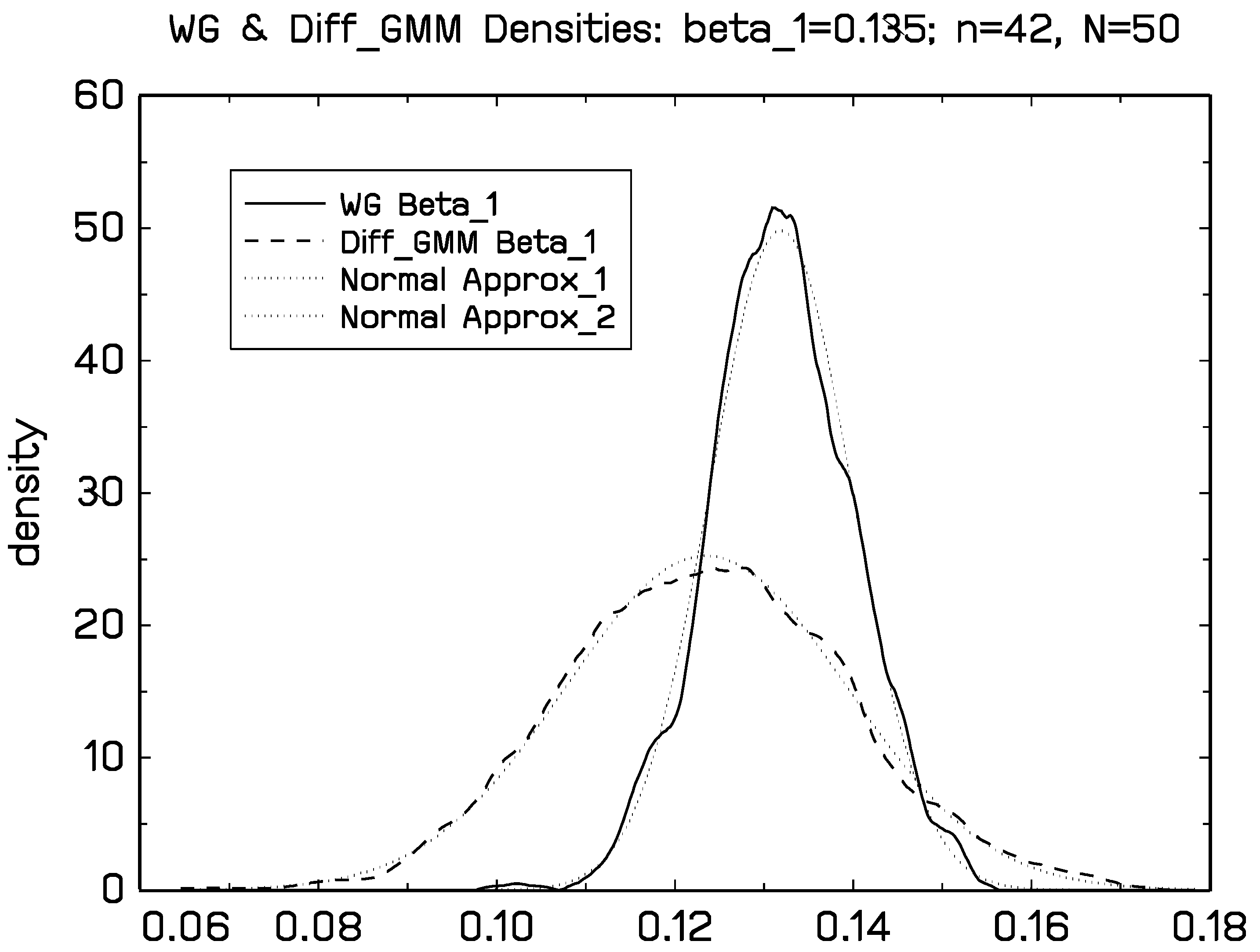
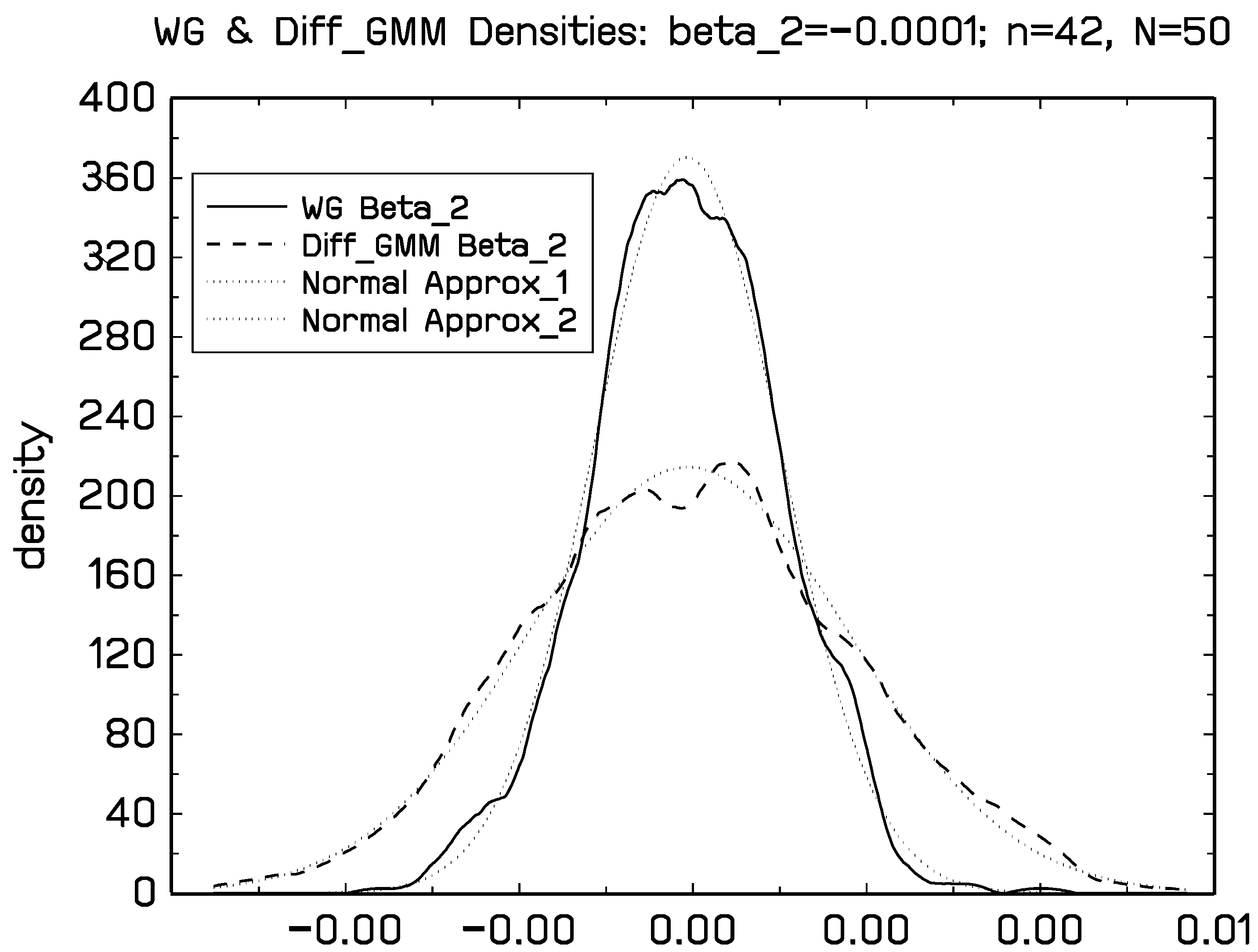
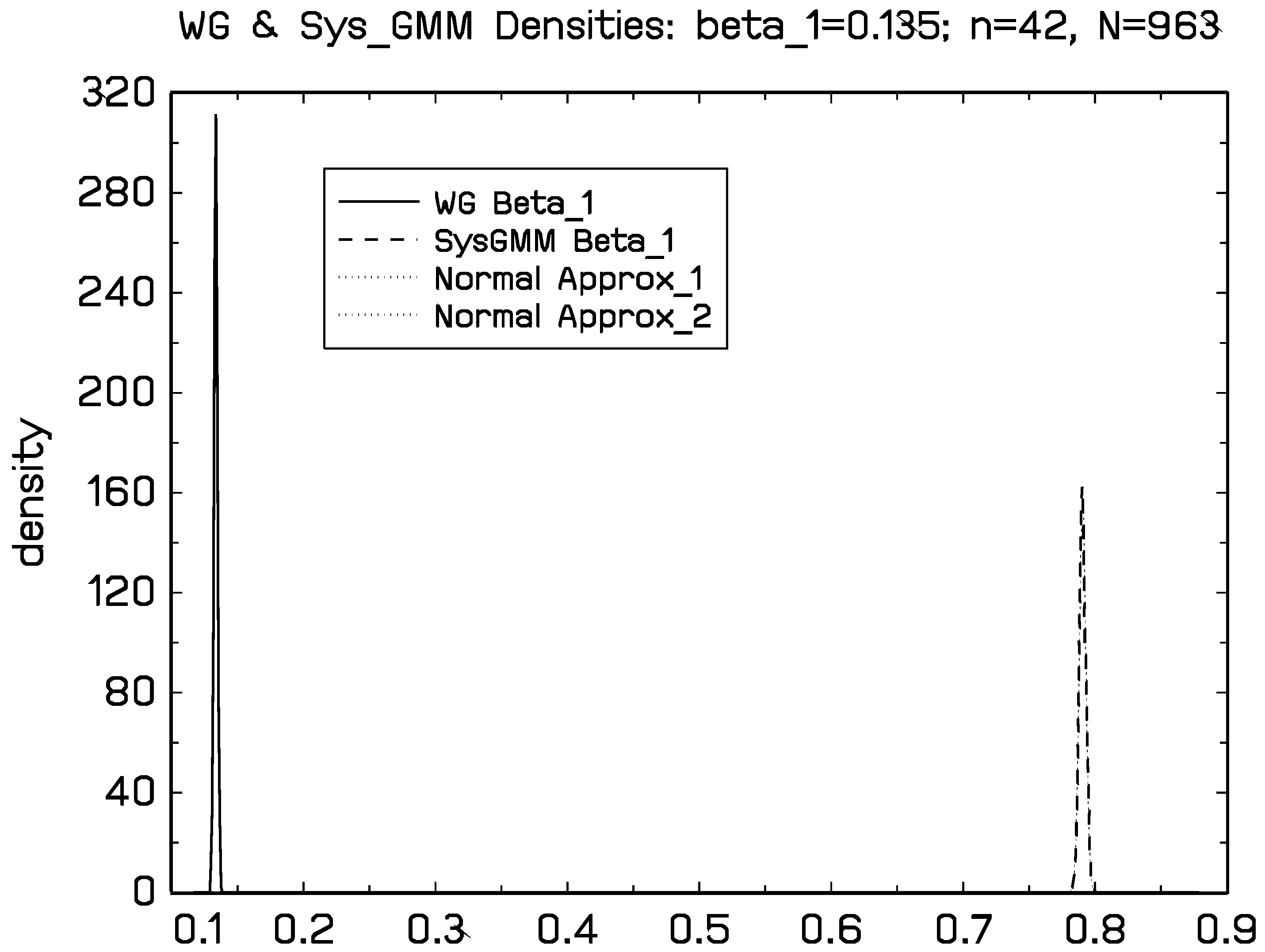
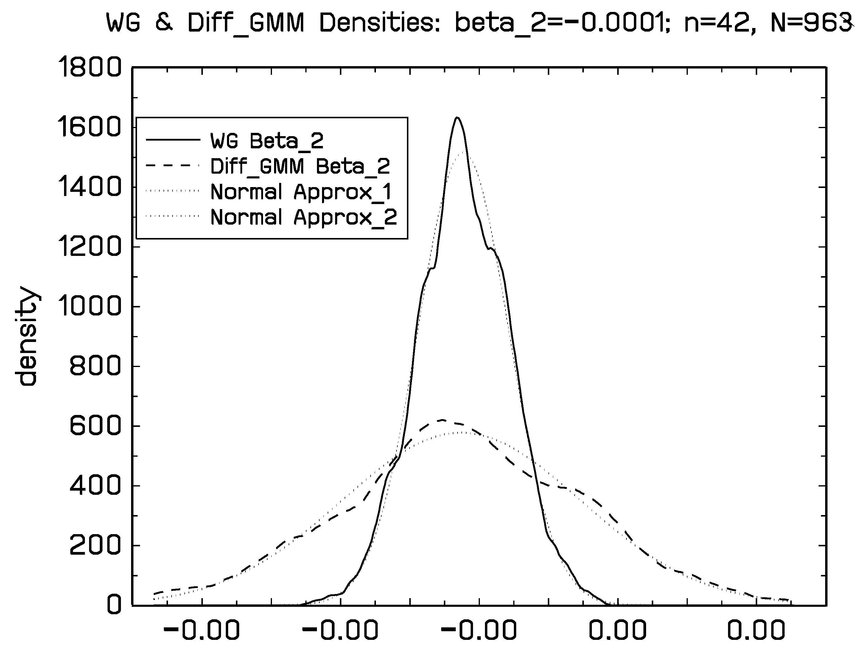
Figure A1, Figure A2, Figure A3 and Figure A4 collected in Appendix A show densities of the WG, diff-GMM, and sys-GMM estimates of the first Equation (40) of this model based on $R=1500$ replications with sample sizes $n=42,$ $N=50,$ using only the first 50 cross section observations of ($R_{it},C{O}_{2t}$)${}_{t=1,i=1}^{n,N}$ and therefore much smaller than the observational cross section sample size $N=963.$ The data were generated as described above with true parameter settings (42) and (43) and observed data for radiation $R_{it}$ and CO${}_2$ equivalent $C{O}_{2t}.$ Simulation results based on the full cross section sample size $N=963$ are reported in the subsequent Figure A5, Figure A6, Figure A7 and Figure A8.

The WG densities show little bias (as might be expected with time series sample size $n=42$) and seem to conform well with asymptotic normality for both ${\beta }_1$ and ${\beta }_2$. The Diff_GMM estimates show little bias in the estimation of ${\beta }_2$ but show downward bias in the estimation of ${\beta }_1$, and have much greater variance than the WG estimates, for both ${\beta }_1$ and ${\beta }_2.$ By contrast the sys-GMM estimates are biased for both parameters. The sys-GMM estimates of ${\beta }_1$ are particularly heavily biased upwards from a true value of ${\beta }_1=0.135$ to a value around unity. The reason is the large ratio

$$r_{\alpha }=\frac{{\sigma }_{\alpha }}{{\sigma }_u}=\frac{7.4147}{0.4929}=15.043,$$

of the standard deviation of the individual effects relative to the equation error. System GMM (both optimal and non-optimal versions) is known to be very sensitive to heterogeneity in the fixed effects ${\alpha }_i$ and, in particular, to the magnitude of $r_{\alpha }^2$ (Hayakawa 2015; Bun and Windmeijer 2010), which in the present case is $r_{\alpha }^2=226.29$. For a simple panel AR(1) model with fixed effects, for instance, Hayakawa shows that non-efficient system GMM is actually inconsistent when $n/N\to c>0$ and the probability limit of the system GMM estimate of ${\beta }_1$ tends to unity when $r_{\alpha }^2\to \infty .$ This analytic finding corresponds closely with the simulation results obtained here for the more complex model (40) and (41) with its multiple sources of nonstationarity.

These simulations confirm the existence of substantial bias in system GMM estimation in the present context. The findings are very similar for the data-realistic sample size setting $N=963,$ although the distributions are much tighter in view of the larger value of the cross section sample size $N.$ Interestingly, the system GMM estimates of ${\beta }_1$ in this case are centered around 0.8 rather than unity, which corresponds closely to the sys-GMM estimate obtained with the observed data where ${\widehat{\beta }}_1=0.864$ (see Table 1). Moreover, since the ratio $\frac{n}{N}=\frac{42}{963}=0.0436$ is close to zero in this case, Hayakawa’s (2015) expression for the bias in his Theorem 4(a) indicates that the bias will be smaller for $N=963$ than when $N=50$ and this analytic result for the bias matches the simulation findings for the temperature data.

6. Concluding Remarks

Panel data econometric methods seem well suited to assess the impact on global temperature of rising greenhouse gas (GHG) concentrations in Earth’s atmosphere. They have the advantage of modeling the aggregate impact of GHG on temperature while also incorporating the effects of changes in downwelling surface radiation at the station level. In this way, panel models may account for some of the observed ‘local dimming’ that has occurred during the past half century due to rising levels of local pollution. Recent work by Magnus et al. (2011) and Storelvmo et al. (2016) sought to model these effects through system estimation of a dynamic panel regression framework, finding that the dimming influence of aerosols on surface radiation masked more than 30% of the aggregate effect of rising CO${}_2$ levels on Earth’s average temperature.

The analytic and simulation results of the present paper show that these local dimming effects are surprisingly robust to the econometric methodology used to estimate Earth’s transient climate sensitivity. Estimates of this aggregate-level parameter are found to be invariant to the dynamic panel regression method employed. However, estimates of some of the individual parameters in the dynamic panel regression system can differ substantially. In particular, system GMM methods are found to be unreliable in estimating the panel autoregressive coefficient and certain aggregate parameters, suffering from considerable bias. Both the simulation and analytic results favor within group methods for time series and cross section sample sizes of the order now available in observed spatio-temporal datasets. Within group panel estimation also gives results that are broadly in line with findings from direct time series cointegrating regressions of the aggregate data. This correspondence between the results of methods that employ disaggregate and aggregate data gives some assurance of the reliability of the estimates of climate sensitivity to CO${}_2$ levels. Some further computations that reinforce some of the present findings about the finite sample performance of dynamic panel regression methods and provide R programs for estimating models of this type are given in Phillips and Han (2019).

References

- Arellano, Manuel, and Stephen Bond. 1991. Some tests of specification for panel data: Monte Carlo evidence and an application to employment equations. The Review of Economic Studies 58: 277–97. [Google Scholar] [CrossRef] [Green Version]
- Blundell, Richard, and Stephen Bond. 1998. Initial conditions and moment restrictions in dynamic panel data models. Journal of Econometrics 87: 115–43. [Google Scholar] [CrossRef] [Green Version]
- Bun, Maurice J. G., and Frank Windmeijer. 2010. The weak instrument problem of the system GMM estimator in dynamic panel data models. Econometrics Journal 13: 95–126. [Google Scholar] [CrossRef] [Green Version]
- Hayakawa, Kazuhiko. 2007. Small sample bias properties of the system GMM estimator in dynamic panel data models. Economics Letters 95: 32–38. [Google Scholar] [CrossRef] [Green Version]
- Hayakawa, Kazuhiko. 2015. The asymptotic properties of the system GMM estimator in dynamic panel data models when both N and T are large. Econometric Theory 31: 647–67. [Google Scholar] [CrossRef] [Green Version]
- Kaufmann, Robert K., Heikki Kauppi, Michael L. Mann, and James H. Stock. 2011. Reconciling anthropogenic climate change with observed temperature 1998–2008. Proceedings of the National Academy of Sciences of the United States of America 108: 11790–93. [Google Scholar] [CrossRef] [PubMed] [Green Version]
- Kaufmann, Robert K., Heikki Kauppi, Michael L. Mann, and James H. Stock. 2013. Does temperature contain a stochastic trend: linking statistical results to physical mechanisms. Climatic Change 118: 729–43. [Google Scholar] [CrossRef]
- Kruiniger, Hugo. 2009. GMM Estimation of Dynamic Panel Data Models with Persistent Data. Econometric Theory 25: 1348–91. [Google Scholar] [CrossRef] [Green Version]
- Magnus, Jan R., Bertrand Melenberg, and Chris Muris. 2011. Global Warming and Local Dimming: The Statistical Evidence. Journal of the American Statistical Association 106: 452–64. [Google Scholar] [CrossRef] [Green Version]
- Park, Joon Y., and Peter C. B. Phillips. 1988. Statistical Inference in Regressions With Integrated Processes: Part 1. Econometric Theory 4: 468–97. [Google Scholar] [CrossRef] [Green Version]
- Park, Joon Y., and Peter C. B. Phillips. 1989. Statistical Inference in Regressions With Integrated Processes: Part 2. Econometric Theory 5: 95–131. [Google Scholar] [CrossRef] [Green Version]
- Phillips, Peter C. B. 2018. Dynamic Panel Anderson-Hsiao Estimation With Roots Near Unity. Econometric Theory 34: 253–76. [Google Scholar] [CrossRef] [Green Version]
- Phillips, Peter C. B., and Chirok Han. 2019. Dynamic Panel GMM using R. In Conceptual Econometrics Using R. Handbook of Statistics. Edited by Hrishikesh D. Vinod and C. Radhakrishna Rao. Amsterdam: Elsevier, vol. 41, chp. 5. pp. 119–44. [Google Scholar]
- Phillips, Peter C. B., Thomas Leirvik, and Trude Storelvmo. 2020. Econometric Estimates of Earth’s Transient Climate Sensitivity. Journal of Econometrics 214: 6–32. [Google Scholar] [CrossRef]
- Storelvmo, T., T. Leirvik, U. Lohmann, P. C. B. Phillips, and M. Wild. 2016. Disentangling Greenhouse Warming and Aerosol Cooling to Reveal Earth’s Climate Sensitivity. Nature Geoscience 9: 286–89. [Google Scholar] [CrossRef]
- Storelvmo, Trude, Ulla K. Heede, Thomas Leirvik, Peter C. B. Phillips, Philipp Arndt, and Martin Wild. 2018. Lethargic Response to Aerosol Emissions in Current Climate Models. Geophysical Research Letters 45: 359–78. [Google Scholar] [CrossRef]