Climate Disaster Risks—Empirics and a Multi-Phase Dynamic Model †

1
Department of Institut für Statistik, Ludwig Maximilians University of Munich, 80333 Munich, Germany
2
New School for Social Research, New York, NY 10011, USA
3
Senior Research Associate, IIASA, Schlossplatz 1, A-2361 Laxenburg, Austria
*
Author to whom correspondence should be addressed.
†
The basic structure of this paper was developed while Willi Semmler was a visiting researcher at the IIASA, Laxenburg, and visiting scholar at the IMF Research Department. The authors would like to thank Chris Papageorgiou, Prakash Loungani and their colleagues as well as Elena Rovenskaya, Raimund Kovacevic and Sergey Orlov for many helpful insights and comments. We are grateful to three anonymous referees for excellent comments on an earlier draft.
Econometrics 2020, 8(3), 33; https://doi.org/10.3390/econometrics8030033
Submission received: 30 January 2020
/
Revised: 31 July 2020
/
Accepted: 7 August 2020
/
Published: 18 August 2020
(This article belongs to the Collection Econometric Analysis of Climate Change)
Abstract
:Recent research in financial economics has shown that rare large disasters have the potential to disrupt financial sectors via the destruction of capital stocks and jumps in risk premia. These disruptions often entail negative feedback effects on the macroeconomy. Research on disaster risks has also actively been pursued in the macroeconomic models of climate change. Our paper uses insights from the former work to study disaster risks in the macroeconomics of climate change and to spell out policy needs. Empirically, the link between carbon dioxide emission and the frequency of climate related disaster is investigated using a panel data approach. The modeling part then uses a multi-phase dynamic macro model to explore the effects of rare large disasters resulting in capital losses and rising risk premia. Our proposed multi-phase dynamic model, incorporating climate-related disaster shocks and their aftermath as a distressed phase, is suitable for studying mitigation and adaptation policies as well as recovery policies.
Keywords:
climate economics; disaster risk; macro feedback; multi-phase macro model; monetary and financial policies; environmental economicsJEL Classification:
C61; Q54; Q58; H51. Introduction
Many recent studies in the economics of climate change have utilized modern statistical and econometric methods to study the links between GDP growth, greenhouse gas (GHG) emission, global warming, and climate-related disasters. Additional research, for example by the IMF (2017), has shown that in particular low-income countries and regions will be vulnerable to climate-related disasters. At the same time they have only little economic and financial capacity to adapt.1
Similar research on large disaster risk has been undertaken in financial economics, especially since the financial crisis 2007–2009 and the subsequent world-wide recession. In particular, the destruction of capital stocks and jumps in risk premia after a rare large economic and financial crisis are investigated in great detail. For example, Rietz (1988) studies rare market crashes and their effect on equity risk premia. Barro (2006) uses as disaster measure the decline of GDP growth, while Barro and Ursua (2008) and Gabaix (2011) investigate the decline of consumption spending due to large disasters. Barro (2006) and Gourio (2012), on the other hand, measure disasters in terms of loss in total factor productivity (TFP) and declines in the capital stock. The latter is formally introduced in these models as a sudden increase in the capital depreciation rate. The proportionality of output and capital losses can then be demonstrated in an “AK” growth model (Barro 2006). Usually strong persistence of disaster shocks is assumed, which results in long-run effects of such shocks; see Catalano et al. (2018). Recent approaches frame this issue in the context of DSGE models.
Gallic and Vermandel (2020) introduce weather shocks affecting land productivity into a small open-economy model. They estimate their model based on data for New Zealand and find that weather shocks can explain business cycle fluctuations to a certain degree. Numerical solution methods for solving DSGE models with disasters—by measuring disasters as physical capital and output losses—have been developed by Fernandez-Villaverde and Levintal (2016). Disasters are then mainly modeled as highly persistent shocks with mean reversion after the event. Economic and financial studies on rare large crashes are undertaken to demonstrate the effects of financial disasters on asset prices and returns. Researchers intend to show that the equity premium puzzle and volatile discount rates can be resolved with reference to rare large disasters.
There is also a significant strand of literature focusing on climate disasters and the physical destruction of countries and regions they cause. The focus lies on the destruction caused by rare large disasters on the one hand and on slow temperature increases—entailing negative long-run productivity effects (IMF 2017)—on the other hand. Particularly important is the study by Burke et al. (2015) which explores the non-linear effects of climate change based on the work of Gumbel (1958). A related study is given by Cantelmo et al. (2017). They introduce climate disaster losses in a macroeconomic model as capital losses, implying some long-run persistent effect. Here, fiscal policy is suggested for disaster management. The role of public capital for disaster management is stressed by Adam and Bevan (2014) and Bevan and Adam (2016).
Although the causes of disaster risk arising from climate change differ from disaster risk originating in large financial crises the effects may be similar. In our analysis, we focus on disaster risk associated with extreme weather events. Batten (2018) points out that the effects of extreme weather events are very similar to economic shocks: they are mostly unpredictable events with potentially significant macroeconomic consequences. In both cases actual output may recover in the short run, but potential capacity is reduced, while physical, public, and human capital will be destroyed. Hysteresis effects of disaster shocks may then cause persistently low future growth rates. In this context, some authors suggest working with multiple equilibria models, allowing for trapping probabilities and poverty traps after the disaster event; see Kovacevic and Pflug (2011) and Kovacevic and Semmler (2020). Moreover, due to large temporary shocks and capital losses, risk premia and borrowing cost are likely to rise steeply. Increased credit constraints will be the result and the affected country or region may face an increased trapping probability, resulting in a very slow recovery only.2
Consequently, both research areas are concerned with similar policies—policies addressing the mitigation and reduction of long-run causes of disasters and how to deal with after-the-event situations. In terms of policies, balancing the competing, yet often complementary, needs of climate change, mitigation and adaptation becomes a complex problem. Different policies may be substituted in the short run, but complements in the long run: active mitigation policies may reduce the risk of large disasters, but they are expensive and their benefits may only accrue in the long run. At the same time, adaptation policies may solve short-term problems in a more satisfactory way, but their costs increase strongly if mitigation policies remain underfunded.
The effects of rare large disasters on risk premia, credit cost, credit spread and credit constraints will be analyzed in the context of our model. In addition, fiscal, monetary and financial policy interventions will be introduced to study disaster management approaches in detail. To the best of our knowledge, this has not been done in climate change-related disaster studies. These are important additional components of policies. Furthermore, they are not only required after climate disasters, but may also become necessary after a pandemic crisis as recently experienced by many countries.
We motivate these important policy issues by exploring the link between rising carbon dioxide levels in the atmosphere and the frequency of climate disasters first. The focus lies on seven regions: East Asia and Pacific (EAS), Europe and Central Asia (ECS), Latin America and the Caribbean (LCN), Middle East and North Africa (MEA), North America (NAC), South Asia (SAS), and Sub-Saharan Africa (SSF). We then present a modeling framework describing the occurrence of large disasters in a multi-phase dynamic macro model. In this context, we also discuss the role of monetary and financial policy responses.
We build on a macro model developed by Bonen et al. (2016), Semmler et al. (2018b) and Semmler et al. (2018a) which allows for studying the issue of large climate-related disaster shocks and climate change policies. Our model explicitly solves for fiscal and financial resources to deal with trade-offs between mitigation and adaptation policies. These policies are operationalized as time-varying shares of public capital in support of carbon-neutral productivity-enhancing infrastructure, mitigation and adaptation capital. In those model variants, carbon intensity of the energy resources is not a side-product of production. Instead, we endogenize carbon intensity by linking emissions to the extraction of a non-renewable resource (e.g., fossils fuels), and show how renewable energy can be phased in through public-sector investment, thereby phasing out fossil fuels. This allows us to combine contemporary ‘social cost of carbon’ (SCC) approaches, as used in an Integrated Assessment Model (IAM), with the resource extraction models of Hotelling (1931) and Pindyck (1978) and extended by Maurer and Semmler (2011). Moreover, the macro model presented here extends the recent modeling advances that allow agents to respond to climate change by combining mitigation and adaptation actions; see Ingham et al. (2007). The solution method of solving the multi-phase model is presented in Semmler et al. (2018b).
From an applied policy perspective, climate-related finance policy—we mainly explore the issue of scaling up climate investment through bond issuance—suggests bond financing at an initial stage. Accumulated debt is then reduced by increases in income taxes. We, therefore, propose combining fiscal, financial, and monetary policies for tackling climate change in a general way. Our approach gives rise to a three-phase model. In the first stage, we suggest using taxation and fiscal tools, followed by scaling up investments by bond financing, concluded by a final stage of bond repayment and debt reduction. A single-stage model is contrasted with such a multi-phase model. We also explore the economic and financial impacts of large disasters and study the impact of fiscal, financial and monetary policy tools on mitigation as well as on adaptation.
The remainder of the paper is organized as follows. Section 2 presents our empirical results on the links between rising carbon dioxide levels—to a large extent due to economic expansion—and the number of climate-related disasters for a given year (disaster frequency). Section 3 introduces the single-phase and multi-phase macro models with phase-specific climate disasters, fiscal, monetary, and financial policies. Section 4 provides some discussion on broader policy initiatives including fiscal and monetary policy tools for mitigation and adaptation. Finally Section 5 concludes the paper.
2. Empirics of Disaster Frequency
In this section, we study the frequency of climate-related disasters and their relationship with GHG emission for seven regions. Our empirical results serve as motivation for the modeling and policy approaches of Section 3 and Section 4.
Detecting systematic changes in climate disaster risks is challenging due to the infrequent nature of disaster events as well as the quality and shortness of disaster records (Stott et al. 2016). Evidence on a link between increases in climate disaster risks and anthropogenic climate change is therefore mixed. Still, a positive relationship between climate change and the occurrence probability and magnitude of disasters is reported in recent “event attribution” studies such as NASEM (2016) and Stott (2016). Our empirical approach is closely related to Thomas et al. (2013) and Thomas and Lopez (2015). They study the increase of climate-related disasters and anthropogenic climate change based on panel models for count data and find a positive relationship between disaster frequency and disaster risk factors caused by human-made GHG emission.
Before going into further details, it is worth contrasting the way probability theory defines (exogenous) rare large events with our set up. Studies based on a probabilistic approach weigh the (low) probability of large disaster events with the size of the losses. In our context, however, we see disaster probabilities being driven endogenously by rising vulnerabilities due to a rise in CO2 emission. Our empirical approach mainly builds on the EMDAT database provided by the Centre for Research on the Epidemiology of Disasters (CRED).3 The database provides observations on different kinds of natural and technological disasters. Following Coronese et al. (2018) we identify six types of natural disasters which are associated with extreme weather effects due to climate change: floods, droughts, landslides, wildfires, storms, and extreme temperature.
As disaster data are known for being subject to several data issues, such as under-reporting for disasters in the more distant past (Guha-Sapir et al. 2013), data preparation becomes a vital issue. We only use data starting in 1976 to deal with the most severe data distortions. In addition, we focus on the number of disasters/disaster frequency.4 Our regional disaster frequency variables are constructed by summing up the number of climate-related disaster for the six categories mentioned above for a given year and region.5
Before studying the relationship between CO2 emission and climate-related disasters in more detail, we present some stylized facts based on the EMDAT database and CO2 emissions data provided by Mauna Loa Observatory.
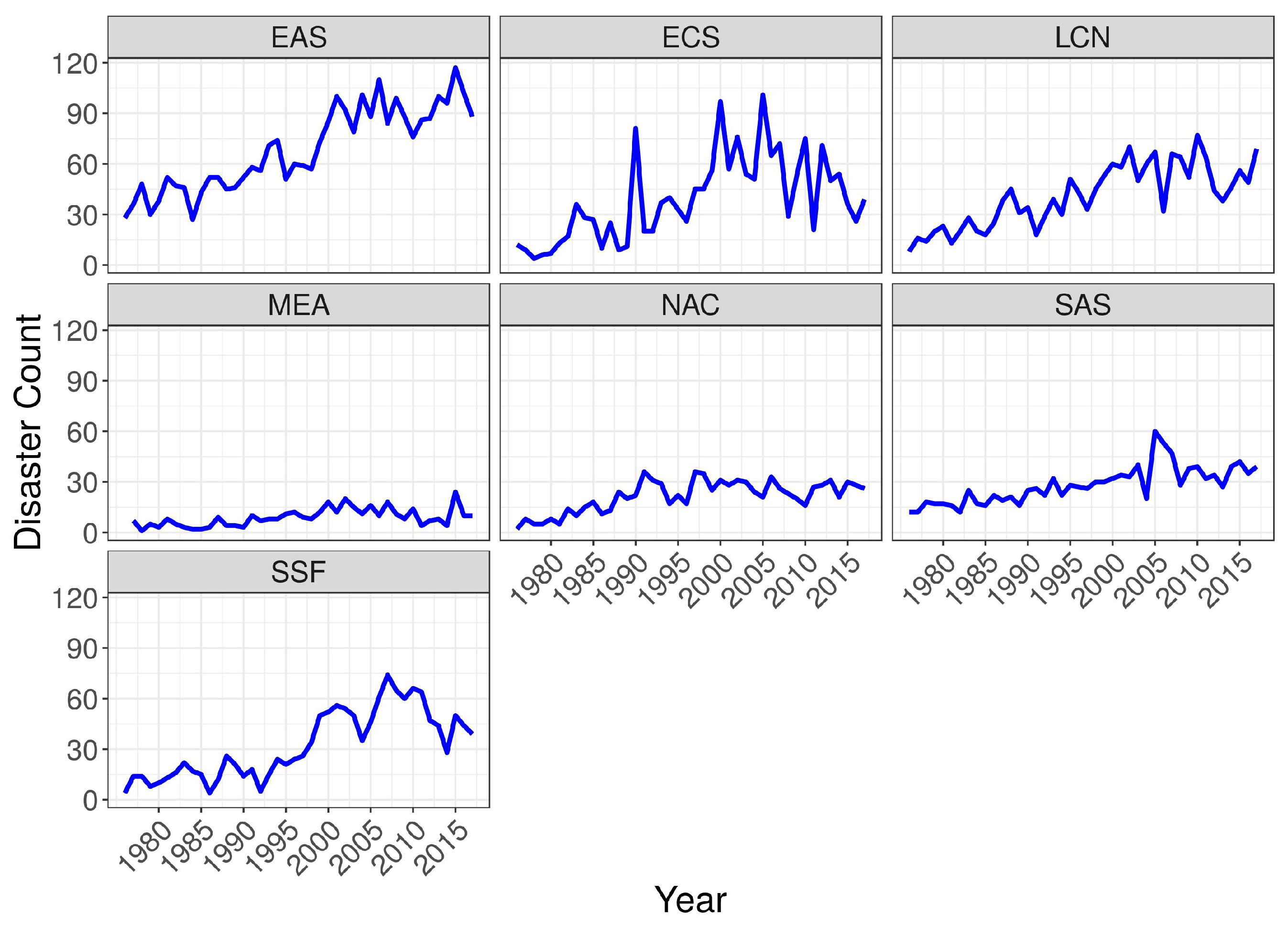
Figure 1 depicts our seven regional disaster frequency time series. We observe a clear upward trend for most regions. In Europe and Central Asia, an upward trend is clearly given up until 2005. In the following years, the number of observations decreases somewhat. On the other hand, the trend for East Asia and Latin America and the Caribbean is increasing over the entire sample period. A similar pattern is observed for Sub-Saharan Africa. Here, a small decrease for the most recent years becomes visible again. The number of disasters decreases from an all-time high of 74 observations in 2007 to 39 climate-related disasters in 2017. In contrast to theses patterns, the trends in the Middle East and North Africa and in North America are not as pronounced, although we observe a positive trend in North America. Finally, in South Asia an upward trend is observed as well.
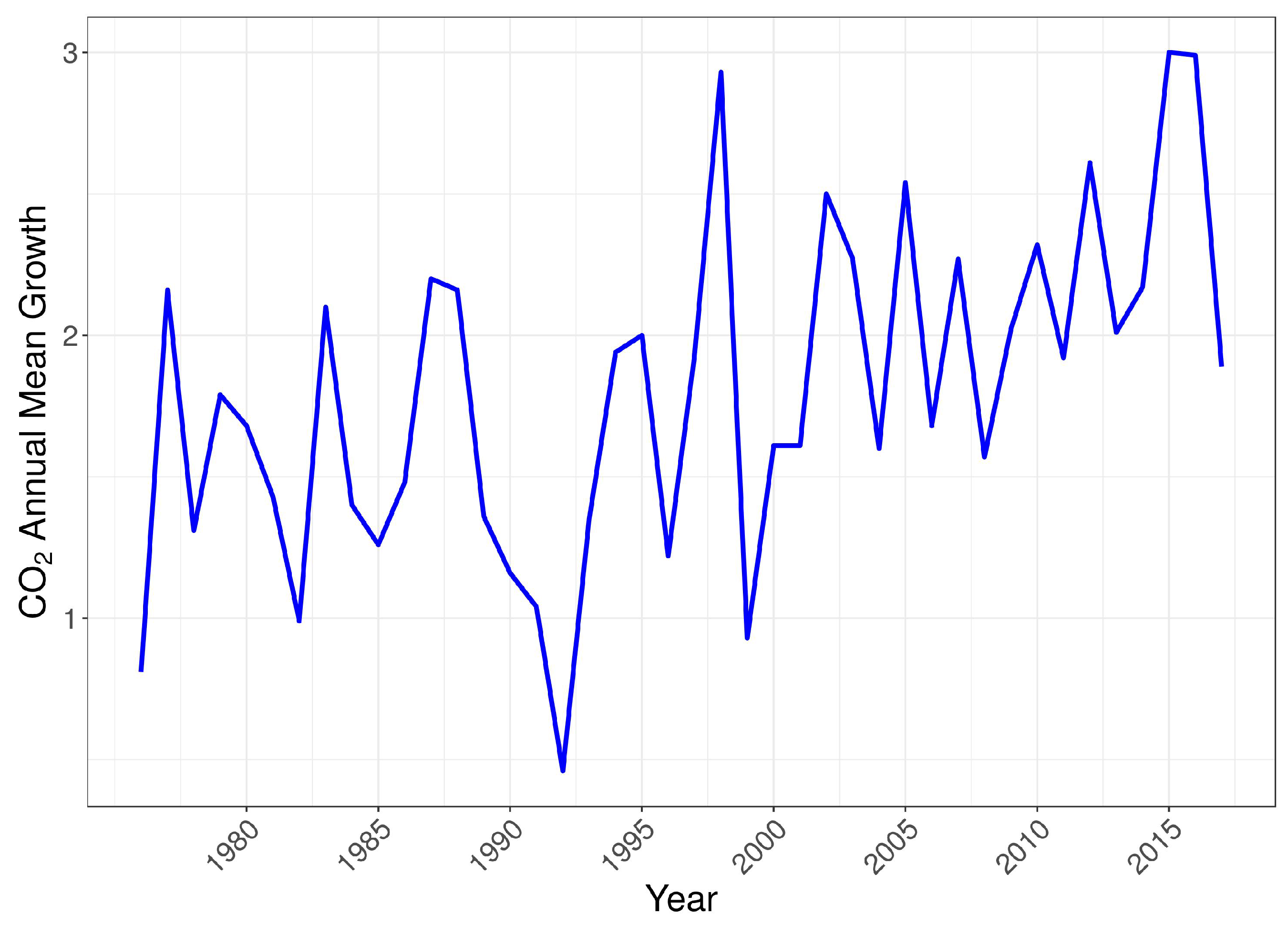
Figure 2 shows the annual increase in carbon dioxide in the atmosphere expressed as a mole fraction in dry air. The data is provided by the Mauna Loa Observatory and shows the growth (first differences) of the collected data between 1976 and 2017. Data collected at the Mauna Loa Observatory is intended to represent carbon dioxide levels in the atmosphere for the northern hemisphere. However, the annual increase based on the Mauna Loa data is very similar to the global annual increase and is therefore used for the southern hemisphere as well in this study.6 In the following empirical analysis we will focus on the data shown in Figure 2 and its relationship with the total number of climate-related disaster, represented by Figure 1.
The link between GHG concentration in the atmosphere in general, and CO2 concentration in particular, and the increased frequency of natural disasters is well-documented; see Thomas et al. (2013) for an overview. IPCC (2012) argue that increased GHG emission, leading to increasing concentration in the atmosphere, alters climate variables, especially temperature and precipitation levels. These changes in climate variables increase the frequency of climate-related hazards. Growth in CO2 concentration in the atmosphere, therefore, only represents an indirect effect on climate-related disasters. However, focusing on CO2 instead of changes in temperature and precipitation has certain merits. As Miller et al. (2014) point out, the increasing concentration of GHG (and aerosols) represents the main perturbation to the earth’s climate. In addition, long-lived GHG like CO2 show only limited geographic variations and can be easily measured at a few sites with low levels of uncertainty. Therefore changes in CO2 concentration lend themselves to the empirical analysis in this section. In contrast, changes in surface temperature (anomalies) show high levels of geographic variation, are more volatile and affected by numerous factors, such as the El-Niño Southern Oscillation, solar variability, and volcanic activity (IPCC 2013; Lean and Rind 2008).7
Table 1 summarizes unit root tests for the number of total disaster for each region. We use several tests including the Augmented Dickey-Fuller (ADF) test, the Dickey-Fuller Generalized Least Squares (DF-GLS) test by Elliott et al. (1996) and the test by Kwiatkowski et al. (1992, KPSS). Furthermore we also account for a possible structural break of the series by applying the test by Zivot and Andrews (2002, ZA). As can be seen from Table 1 the test results are not unambiguous. The KPSS test rejects trend stationarity in favor of a unit root process at the 5% significance level for all regions but East Asia and Pacific, South Asia, and Sub-Saharan Africa. For Sub-Saharan Africa, the null hypothesis is rejected at the 10% significance level. The ADF-tests do not reject the null hypothesis of a unit root process, while the DF-GLS unit root test with trend delivers results similar to the KPSS test: the null hypothesis of a unit root is rejected for East Asia and Pacific at the 5% significance level and for South Asia at the 10% significance level. Moreover, we apply the test by Zivot and Andrews (2002) to allow for an unknown break in the trend (ZA Test Trend), the intercept (ZA Test Constant), and in trend and intercept (ZA Test). Test ZA Test rejects the null hypothesis of a unit root for Europe and Central Asia, North America, and South Asia at the 5% significance level. Lastly, we also apply the unit root tests of Table 1 to our atmospheric CO2 levels series. The KPSS test rejects trend stationarity for atmospheric CO2 levels. The other tests do not reject the null hypothesis of a unit root process.
Although evidence on the existence of a unit root for disaster frequency is not clear-cut, we test co-integration between disaster frequency and CO2 concentration based on the test by Engle and Granger (1987). However, the number of observations is limited and test results remain inconclusive as can be seen from Table 2. We observe a highly significant cointegration relationship between disaster frequency and CO2 levels for East Asia and Pacific, Latin America, and South Asia. The relationship is also significant at the 5% significance level for region Middle East and North Africa and Europe and Central Asia. For North America and Sub-Saharan Africa, on the other hand, the test statistic is not significant at the 10% significance level.
In our econometric specification, we account for a possible long-term impact of CO2 levels on disaster frequency: the number of observed disasters for a given year is regressed on the growth in CO2 levels for the same year and lagged growth of CO2 in the atmosphere. More specifically, we use the current and the 17 most recent lagged changes of CO2 in the atmosphere to take the uncertainty regarding the long-term impact into account in our regression. However, as the number of observations is very limited, we sum up the changes of CO2 in the atmosphere into a single regressor labeled Sum of CO2 increases in Table 3 and Table 4. By using current and lagged increases in atmospheric CO2 from the Mauna Loa Observatory as a proxy for the global average, Sum of CO2 increases represents the sum of all CO2 added to and removed from the atmosphere for a given year by human activities and natural processes.8
In Table 3, we report the results of linear fixed-effects panel regressions with individual effects (i.e., regional effects) to control for contemporary regional change. More specifically, we estimate the following model:
where represents total disaster frequency for year t and region r. Vector is given by with being the disaster frequency of the previous year for a given region and representing variable Sum of CO2 increases. Lastly, stands for the regional individual effect.
As increases in CO2 do not vary between regions for a given year, time fixed-effects cannot be applied in our panel regression. Standard errors are clustered on the regional level and corrected for the small sample size. We observe a positive influence of increases in CO2 on the frequency of natural disaster (column Complete Data-Set).9 In addition, we also estimate the same model for large disasters only (column Large Disaster Data-Set). Following Thomas and Lopez (2015) we only retain disasters which affect at least 1000 people or lead to 100 deaths in this specification. As can be seen from the column Large Disaster Data-Set, the result of the now unbalanced panel confirms the result of the previous model. Although we observe the Sum of CO2 increases coefficient decrease in size in the second panel model, it remains positive and statistically significant.10
As discussed above, evidence on co-integration between disaster frequency and CO2 is inconclusive for our data. Therefore, we also estimate the panel model with the change in disaster frequency as the dependent variable. The right-hand side variables do not change and the model can therefore be written as:
The results of this estimation are reported in Table 4. Once again, we observe a positive relationship between increases in CO2 concentration in the atmosphere and (change in) the frequency of disasters.
3. Single- and Multi-Phase Climate-Macro Model
Next, we want to elaborate on how a disaster phase can be built into a climate-macro model. For this purpose, we present first a single-phase base-line climate-macro model that exhibits some essential features of the dynamic climate-macro interactions. Though it is in the spirit of an IAM, it is rather based on a larger scale macro model with fossil resource extraction, green capital, and mitigation and adaptation policies using tax and credit finance of climate policy instruments.
We then extend this type of model to a multi-phase model where one of the phases represent a disaster period after a severe disaster shock. The dynamic multi-phase macro model focuses on the causes and effects of rare large disasters. The disaster phase builds on earlier small scale models which allowed for thresholds and poverty traps, such as Azariadis and Stachurski (2005) and Semmler and Ofori (2007). We permit for shifts into such a phase characterized by a persistent disaster regime. This will allow us subsequently to include considerations pertaining to climate-related monetary and financial policies.
3.1. Single-Phase Macro Dynamic Model
The dynamic climate-macro model should trace the following linkages: economic growth leads to the extraction and use of fossil fuel resources, which will give rise to CO2 emission, leading to temperature increases and eventually reducing economic growth and economic welfare. Mitigation and adaptation policies may be pursued more or less successfully by fiscal and/or financial instruments. Those are activated by the public sector and public capital. However, the rise of debt-financed mitigation and adaptation policies may raise the issue of sustainable debt which has to be controlled for.
Those features are embodied in the following a baseline one-phase model that extends the common IAM but can be turned into a multi-stage model in Section 3.2 and numerically solved in Section 3.3. Our extended integrated assessment model11, here defined as one-phase model, has five state variables.
where K is private (green) capital, R is the stock of the non-renewable (fossil fuel) resource, M is the atmospheric concentration of CO2, b is the government’s debt, and g is public capital. The dynamic system of the extended IAM is defined according to
The decision variables, control vector, are given by
where C denotes consumption, is tax revenue, and u is the quantity of the resource R extracted each period.
The first dynamic in Equation (4) is the accumulation rate of private (green) capital K that produces renewable energy and which drives output by the CES production function,
where A is multifactor productivity,12 and are efficiency indices of private capital inputs K and the extraction rate of (non-renewable) fossil fuel energy, u, respectively. In Equation (4), private-sector output Y is modified by the public infrastructure share allocated to productivity enhancement , for . This public–private interaction generates total output as from which the economy consumes C, pays taxes , and is subject to physical depreciation, , as well as demographic depreciation, n. The exponent is the output elasticity of public infrastructure, . The last term in Equation (4) is the opportunity cost of extracting the non-renewable resource u, where and are the scale and shape parameters that tie the cost of u to the remaining stock of the resource as in Hotelling (1931).
Equation (5) indicates the stock of the non-renewable resource R, which depletes by u units in each period. The non-renewable resource emits carbon dioxide and thus increases the atmospheric concentration of CO2 at rate in Equation (6). The stable level of CO2 emissions is of the pre-industrial level , which is naturally re-absorbed into the ecosystem (e.g., oceanic reservoirs) at rate . The last term in Equation (6) is the reduction of per-period emissions, , due to the allocation of of public capital g to mitigation projects.
The last two dynamics are the accumulation of debt b and public capital g. In Equation (7) public debt grows at the fixed interest rate , and is serviced with the share of tax revenue not allocated respectively to capital accumulation, , social transfers, , or administrative overhead, . Thus, . Equation (8) states that the stock of public capital, or total infrastructure, evolves according to the allocated tax revenue stream and funds paid in from abroad, (it may represent donations from outside donors). For developed countries, we may assume , but may be the case for many developing countries. Lastly public capital, g, depreciates by and is adjusted for population growth, n.
We assume throughout that the public capital allocations satisfy
We could either take fixed values for or we may consider the allocations as additional control variables. We opt for the first option and take parameters as given.
Using the state variables, , and choice variables, , we can write the dynamics (4)–(8) in compact form as
The initial state vector will be specified later. To this system we may want to add the terminal constraint
the control constraint
and the pure state constraint
The terminal constraint restricts the final level of the capital stock to a predetermined non-negative value, the control constraint determines an upper bound for the extraction rate, and finally the state constraint places an upper cap on the total level of CO2 in the atmosphere for each period of time.
Next, we define the objective function, i.e., the social welfare function. We use it with a finite decision horizon. It is to be maximized over a given decision horizon , where denotes the terminal time:
The welfare function in (16) is isoelastic with four input components all in per capita terms: (i) consumption C, (ii) the share of tax revenue used for direct welfare enhancement (e.g., health care), (iii) atmospheric concentration of CO2 M above the pre-industrial level , and (iv) the share of public capital g allocated to climate change adaptation. Restricting the exponents ensures social expenditures and adaptation are utility enhancing, and that carbon emissions directly reduce utility. This approach differs from other models that map emissions to temperature changes and then to reduced productivity-cum-output. We believe the direct disutility approach better captures the wide ranging impacts of climate change that may include health impacts, ecological losses and heightened uncertainty, in addition to reduced productivity which may show up in the term A. Finally, note that the discount rate is adjusted for the population growth rate, n, by subtracting it from the pure discount rate, . This step becomes necessary as all values are normalized by population size.
To summarize, our model gives rise to a finite horizon optimal control problem, where the social welfare Equation (16), is maximized subject to the dynamic constraints (12) and the terminal, control and state constraints (13)–(15). This single-phase model can be solved by AMPL.13 Regarding the multi-phase model, the solution procedure has to be augmented by an additional algorithm—explained in detail in Semmler et al. (2018b)—which facilitates finding solutions for models with multiple phases. The algorithm also allows for differences in objective functions and state variables between phases.
3.2. Multi-Phase Dynamic Macro Model
As mentioned before the multi-phase model can be related to earlier small scale model variants which allow for thresholds and poverty traps, such as Azariadis and Stachurski (2005) and Semmler and Ofori (2007).14 In the earlier, simpler models increasing returns to scale, financial market and financing constraints, insufficient insurances with high deductability, and migration of skilled labor and entrepreneurs lead to economies ending up in poverty traps.15 Those feedback effects may result in prolonged disaster phases and very slow recovery phases. A similar scenario will be shown to occur in our multi-phase model. We build on the single-phase baseline model of the previous section and introduce a phase of a prolonged disaster. Strong feedback effects may then lead to a decline in economic growth and lock-in in a (persistent) disaster regime.
Following the literature on large financial crises, e.g., Barro (2006), in a stochastic setting, we can allow for small variations around some original model variables. A level shift may then occur due to a large disaster shock. Subsequently, the model variables are evolving again perturbed by small shocks. In either case, small shocks before and after the level shift do not affect the solution of the model. Only the level shift needs to be taken into account in the solution procedure. Similar to recent approaches in the financial crisis literature, the level shift can be perceived as a downward movement in the deprecation of private and public capital and jump in credit risk premia. A shift into such a model phase, characterized by a persistent disaster regime, might be reversed through some policies at a later point in time. The resulting multi-phase model with a shock as level shift leads to a tractable numerical problem.
This type of extended dynamic macro model maintains the linkages discussed above; economic production and growth lead to the extraction and usage of fossil fuels, which will give rise to CO2 emission, increased disaster risk and damages.16 These effects will reduce economic growth and economic welfare. Mitigation and adaptation policies may be pursued by monetary and financial instruments. Those are activated by the public sector and the monetary authority. Yet, the rise of credit and debt-financed growth raises the usual question concerning sustainable debt which has to be controlled for in the long run.
In our three-phase model, the overall nexus is maintained, but split up into three phases. The first phase of our model can be considered as a stage of mitigation and adaptation policy financed through taxation, similar to a single-phase base-line model. We model a second phase with alternative specifications—small and large disasters reducing capital stocks and increasing risk premia for credit financing. To obtain some robustness results, we focus on model versions with different types of shocks, implying disasters of different impact sizes. In the model, we admit that adaptation policies can reduce vulnerability and thus reduce the occurrences of extreme events. Still, the occurrence of such an event will give rise to a multi-phase model.
As already mentioned, in the first stage the model is exactly the same as the single-phase model of the previous section. The overall objective function is given again by Equation (16), but note that in general the state and control variables in the objective function may change significantly, due to phase shifts. Furthermore, the objective function is now subject to the following dynamics:
In contrast to the single-phase model, a second stage—caused by a possibly large disaster shock inflicting persistent capital losses17—is explicitly modeled here. The strong disaster shock, for example, is modeled by defining jumping from to .18 We also account for a jump of the risk premium, moving from to . We allow for a weak shock as well and compare the effects with the strong shock. Table 5 lists the parameters for both types of shocks. For weak shocks, the depreciation shocks for public and private capital are smaller in phase two. In addition, risk premia are also smaller in the weak shock scenario, in particular in phases two and three.
Although there is some mitigation and adaptation policy in the first stage only now, in the second stage, additional credit (bond) financing will be added, affecting the debt dynamics in Equation (20) but providing also additional finance in Equation (21).
In the third stage, again with the same objective function (16), we have no additional bond issuing any longer. Bonds are paid back by a tax rate on income, but the economy might face some persistent effects on their risk premia. Thus in the third phase the state equations are subject to the following dynamics:
In the third stage, however, capital losses do not occur any longer, but the previous increase in leveraging of private and public capital might still lead, in the case of the strong shock, to a considerably high-risk premium of . We assume here that the risk premium could have been lowered by monetary policy, but would still be high due to the aftereffects of the disaster shock. By way of exemplifying our three-phase model, we pre-fix the first period from to , the second period from to , and last period until .19
3.3. Results of a Three-Phase Model
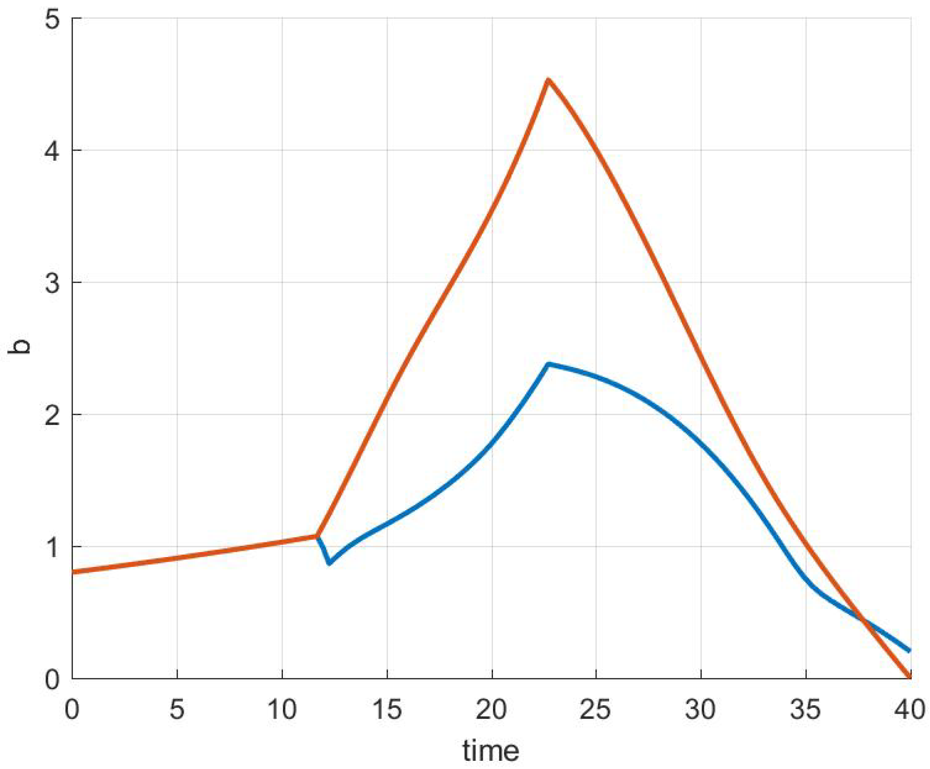
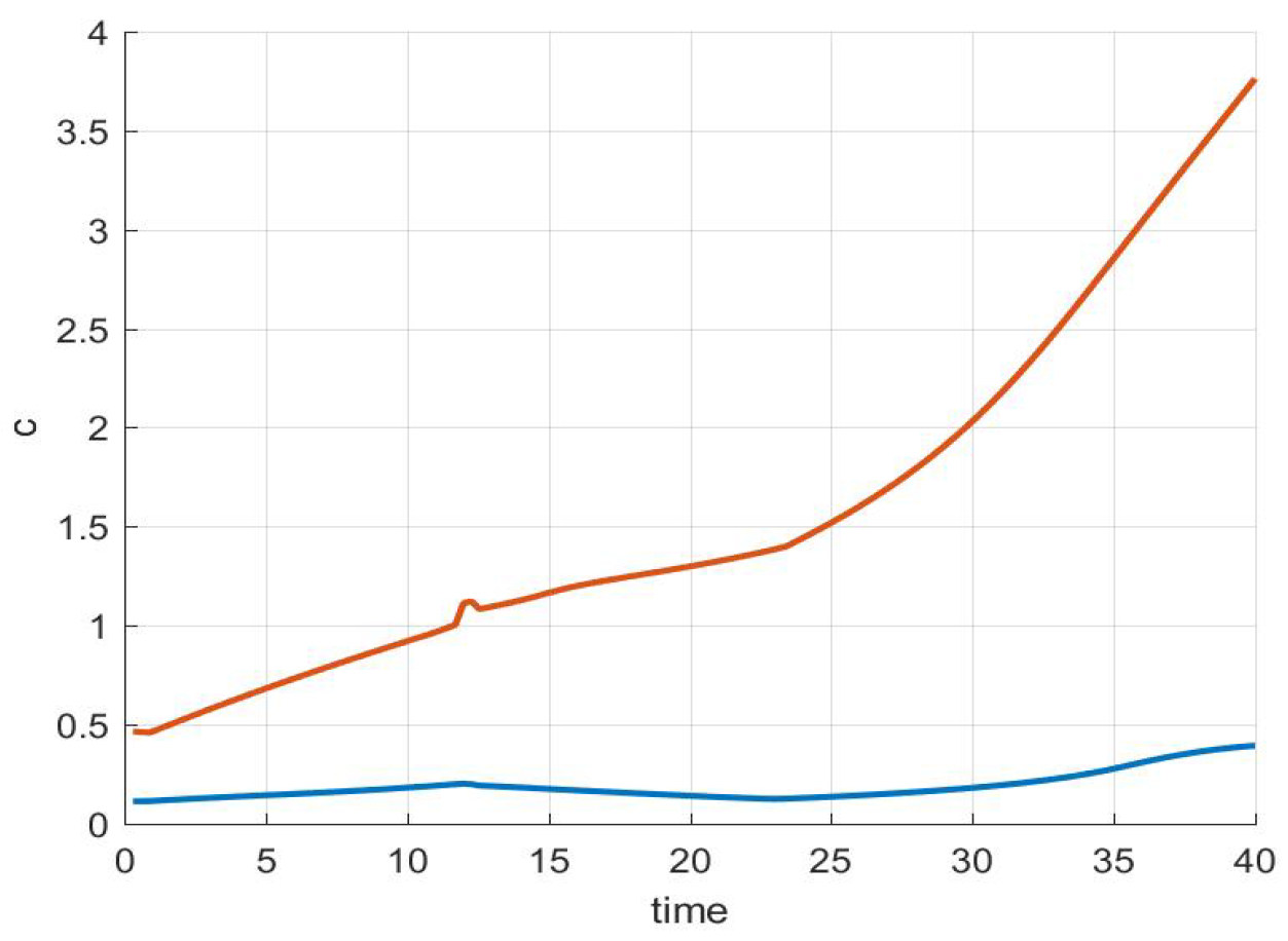
The parameter shifts of Table 5 are used in our subsequent simulations. The effects are drawn in red for weak shocks and in blue for strong shocks. Note that overall, for all variables continuous growth is more successfully achieved without strong shocks. Overall, looking at Figure 3, Figure 4, Figure 5, Figure 6 and Figure 7, we observe that the red line is (except for the fossil fuel resource and stock of CO2) above the blue line.
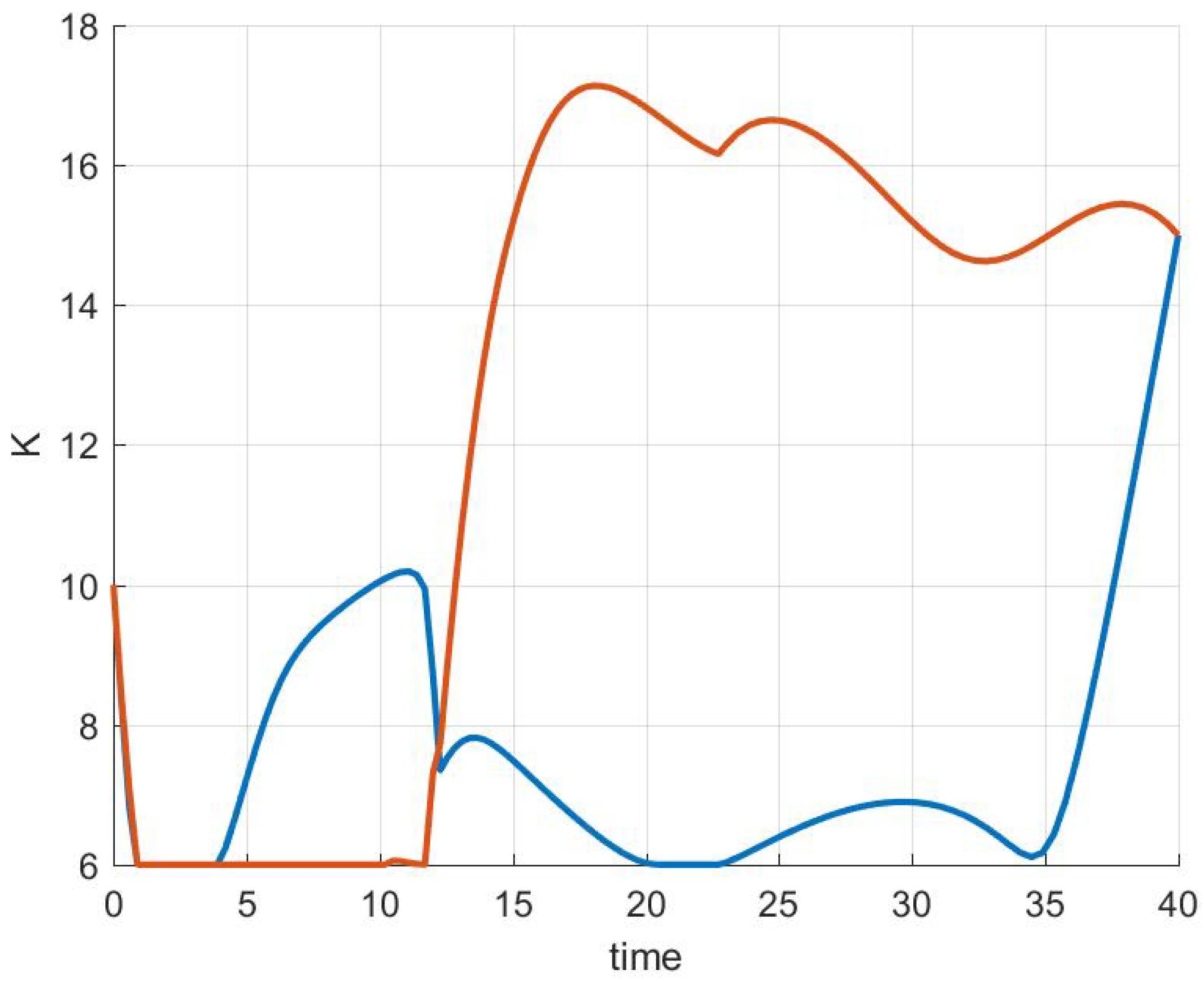
Note that in the Figure 3, Figure 4, Figure 5, Figure 6 and Figure 7 the red line being above the blue line holds for consumption, private capital and public capital stock. This implies that for a small shock, the economy can continuously grow with high borrowing, financing climate related infrastructure investments, and appropriate mitigation and adaptation policies. Thus, to overcome negative externalities, arising from CO2 emissions due to production, there is also a strong evolution of debt, associated with co-financing the mitigation and adaptation policies. With this prolonged growth process, we can also observe a strong extraction of fossil fuel and a build-up of a stock of CO2 emission (which is however counteracted through the climate policy measures).
Yet, with a stronger disaster shock occurring, represented by the parameters of the strong shock in Table 5, which generates a significantly stronger and longer disaster period, consumption stays low, private and public capital stock stays low and so does debt. Consequently, because of lower growth and a smaller increase of capital stocks, the extraction of fossil fuel and the stock of CO2 emission is declining. This result is in line with empirical studies. For example, Cohen et al. (2018) show that in times of a negative output gap emissions are declining.
Looking at details of Figure 3, Figure 4, Figure 5, Figure 6 and Figure 7 we observe in Figure 3 that although stronger disasters generate lower debt, they also generate smaller expansions of capital stocks, and much lower consumption levels. On the other hand, for weaker shocks more effective mitigation and adaptation policies, through the usage of financial sources, , with the aim of preventing disasters generate higher debt, but lower debt to capital ratios and higher welfare levels. For strong shocks debt is rising steadily since risk premia are relatively high. Although public and private capital rise in phase one, both are suffering from the disaster shocks in phase two.
Though debt is still rising, see Figure 3, given the persistent disaster effects20 public and private capital is damaged and we see their size shrinking after 13 periods (see Figure 4 and Figure 5). As a result of strong shocks, allocation towards investment in private capital, K, readjusts, as the second phase—with green bond issuance—nears; see Figure 5. Yet in the period after capital stocks fall. Yet, this is not so for a weak shock where capital (and consumption) are rising.
For a strong shock, both, g and K, decline in the second period; they remain low as long as the disaster effects persist. Only in a later stage public and private capital are recovered; see Figure 4 and Figure 5. The rise of public and private capital in this later period is due to additional bond financing accelerating mitigation and adaption initiatives. Note that in the third phase, the repayment stage of bonds, through income taxes , sets in. For a weak shock both private and public capital stay high.
With our initial conditions, the plots in Figure 6a remain constant after the first phase, while the stock of emitted M becomes high (Figure 6b), in particular for weak shocks, which entails a negative externality; a destructive effect on welfare. Note also that the vulnerability of disasters is reduced with greater public capital; see Equation (16).
Thus, when the level of the stock of CO2 emission, M, becomes high, welfare of households is reduced; see Equation (16). The result of a rise of private (green) capital and public capital supporting the increase of mitigation effort and renewable energy, is preventing the stock of fossil fuel to be extracted to a greater extent. We observe this pattern until , in particular for weak shocks and continuous growth, with both K and g building up, as depicted in Figure 4 and Figure 5, in the second and third period. On the other hand, for a strong shock, Figure 6b shows that the CO2 emission is only rising slightly and the stock of fossil fuel energy (the trajectory in Figure 6a) is only falling slightly and much fossil energy remains unexploited.
Turning to the welfare implications of the disaster shock effects on consumption in the three-stage model, Figure 7 illustrates the results. Unlike in a model of a single-phase, see Semmler et al. (2018b), where naturally consumption continuously rises without disruption (no disaster occurrence), in the current disaster-driven multi-phase model there are intertemporally considerable consumption losses which will only rise slightly when CO2 emission is reduced and the stock of private (green) capital is rising again. Our computed value functions show that welfare in case of weak shock is , and in the case of a strong shock, we have .
Regarding debt sustainability, we see that in terms of the debt-to-capital-stock ratio, , the ratio is higher for strong shocks compared to weak shocks , although debt levels are increasing more strongly in the weak shock scenario, as shown above.
Note that in our proposed framework, emissions are modeled as having direct (damaging) effects on welfare through our objective function given by Equation (16). This formulation encapsulates the multitude of economic, health, migration, and intrinsic environmental losses expected from insufficiently abated climate change in a sensible way. The model also incorporates societies’ adaptive responses to climate change through the use of public funds and credit flows to alleviate the disutility of emissions. In our three-phase model, rare disasters and long-run gradual effects can be studied which are likely to have a considerable effect on productive capacity such as physical, infrastructural and human capital. In particular we have studied the effect on consumption, as shown in Figure 7.
3.4. The Use of Bond Financing
In general, however, even with active fiscal and financial policies, consumption may fall due to externalities from economic activities, entering as disaster risk in the welfare function. Let us specifically look at financial markets and credit flows. The amplified disaster risk and actual disasters affect private and public capital stocks directly. In particular, risk premia are affected detrimentally. On the other hand, the recovery can be accelerated by the support of climate bonds and reduced credit constraints and risk premia. Thus, due to bond issuance—bonds that have to be repaid later on by an income tax—output, private and public capital and consumption, can rise again after the disaster stage. As discussed before, bond issuing has significant benefits since it helps to scale up mitigation, adaptation, and recovery policies.
We build heavily on the financing tools such as (long) maturity bonds here. Though details on such financing mechanism are discussed in Flaherty et al. (2017) and Gevorkyan et al. (2016), we want to highlight a few specifics and practical dimensions relevant in our three-phase modeling context. We have argued that credit (bond) financing allows for better control and scaling of climate policies. Thus financing mitigation and adaptation policies, as well as financing recoveries after disasters, is improved by bond financing.
With respect to mitigation policies, bond financing can stimulate the deceleration of greenhouse gas emissions in a timely manner. It also allows for energy efficiency, changes in energy mix in industrial production, services, transportation, and food production, and permits the development of new renewable energy sources, energy transportation grids, and infrastructure networks.
Regarding adaptation, it can provide funds which can help in reducing frequency and severity of disasters, assist in the reduction of extreme events which arise from increased local frequency—and possibly severity—of storms, coastal flooding, droughts, extreme temperature events, and helps reversing slow long-run impacts from extreme weather events, global water cycles, deterioration of air quality, oceanic warming, shrinking of sea ice cover, deterioration of snow cover and glaciers, and sea-level rise. It could also be used for building up early warning systems—which has been done with respect to financial crises—but which could also act to reduce vulnerability in the case of climate disasters (Thomas et al. 2013).
Bond financing can also be used for climate-related infrastructure concerning the above-suggested green mitigation and adaptation policies as well as for sustainable water management, sustainable land use, biodiversity conservation, grids for renewable energy, clean transportation, and protection of coastal and other areas from flooding and destruction, thus also reducing vulnerability.
Bond financing is likely to be less efficient for recovery policies, but it is expected to be very effective in rebuilding public infrastructure. Other monetary and credit policies are likely to be more suitable as recovery policies. These will be discussed below.
Concerning types of bonds there are government-backed bonds and a variety of municipal government bonds, for example for investments in renewable energy projects, and green bonds issued by the business sector. Often these are asset-backed securities which are similar to traditional bonds by generating some future revenue stream. Covered bonds are a type of asset-backed security that are guaranteed by the issuing agency. Bonds could also be bundled, as soft and hard bonds, and low and high-risk bonds, that might be packaged and sold as investment vehicle– though given some recent experiences the latter might be limited.
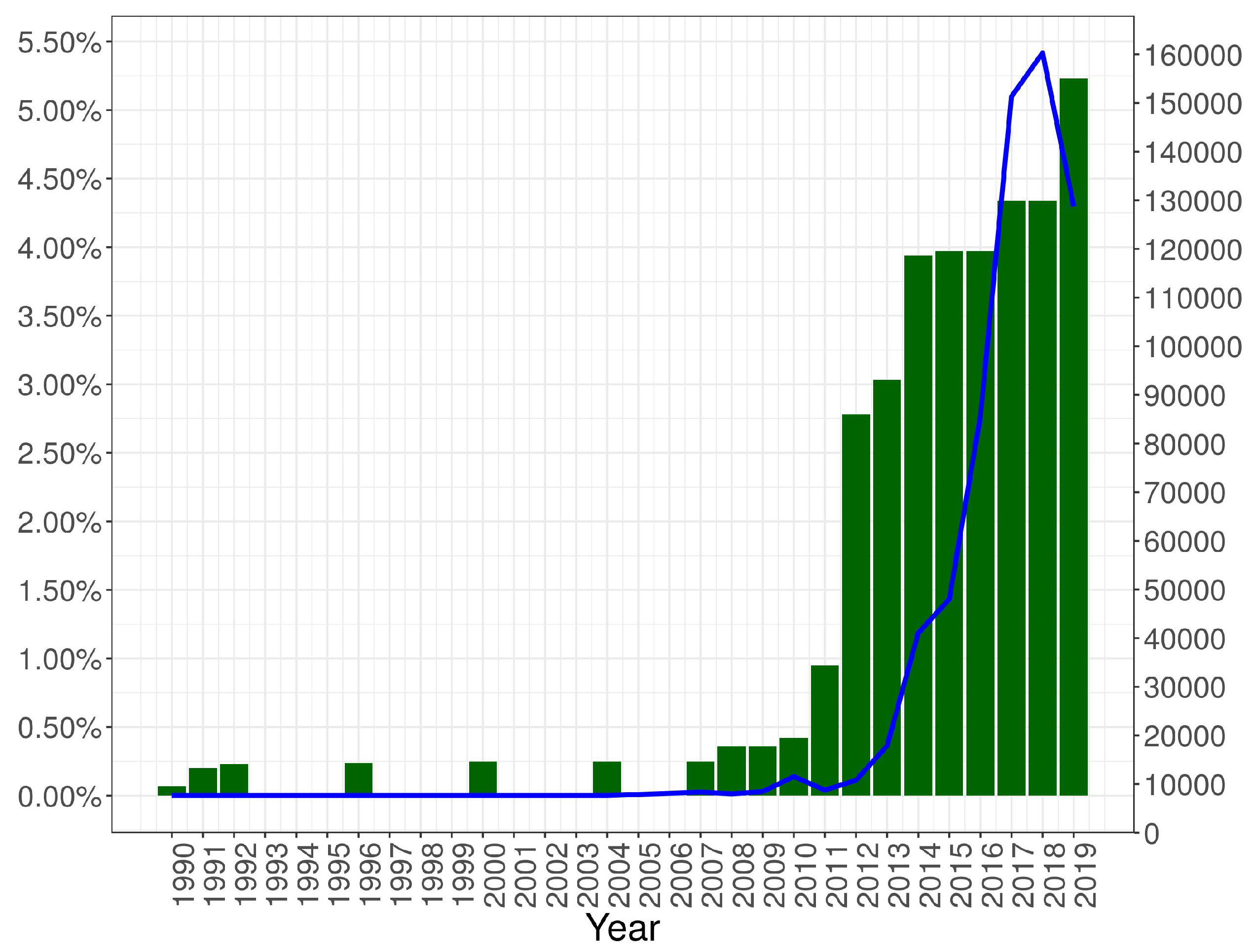
Various types of agencies have been actively providing bond financing. Agencies issuing green bonds fall into three general categories: private businesses, governments and municipalities, and multilateral agencies. The particular bond characteristics tend to vary by type of issuer. Numerous municipalities in developed and developing countries have turned to green bonds as a means of raising green funds. Some investment banks and other financial institutions have also taken note, and have introduced green bonds as part of their offerings. There are also multilateral agencies issuing green bonds, for example, the World Bank, which substantially helped to fund climate policies through issuing bonds for developing countries.21 The number of green bonds issued, as well as the proportion of global GHG emissions which are covered by carbon tax policy, has thereby increased dramatically in recent years. Figure 8 shows this development since 1990.22 The Figure shows that both series have been growing strongly in recent years: starting between 2011 and 2013 we witness a clear upward trend for both series as more and more countries are introducing carbon tax policies to tackle climate change.
Lastly, one might ask whether the current macro and monetary policy environment might be conducive to phase in such green bonds? In particular, long-maturity bonds, because of low- interest rates, low-risk premia and low expected inflation rates should make long-term bonds a good sell. Furthermore, bonds are now largely inflation-adjusted, such as US TIPS to protect long term bonds. It is expected that the current and future interest rates will stay low for quite a while and this, together with low term premia, and low expected inflation rates, is likely to keep the expected future term structure flat.
Concerning the buyers’ side—households’ preferences for those bonds—it looks certain that green bonds will be considered safe long term assets for households, whereas assets from fossil fuel appear to be stranded assets, possibly triggering financial meltdowns; see Battiston et al. (2017). On the other hand, world-wide, funds of $80 to $100 trillion or even more are available as part of large scale portfolios of wealth funds, university endowments, insurances and pension funds and they could include climate bonds as part of their portfolio.
4. Other Policies for the Green Transition and Disaster Management
Mitigation and adaptation policies and disaster risk prevention and recoveries may also be supported more directly by monetary policy. Important aspects of the use of monetary policy in support of climate policy are discussed in Fratzscher et al. (2017), McKibbin et al. (2017), and Monnin (2018). The latter also includes a discussion on the role of the financial sector at large, including banks and central banks.23
Monetary polices could also be more supportive with respect to climate bonds. For example, if central banks accept green bonds as collateral, they could stimulate climate finance. There is some virtuous cycle: Central banks prefer rated bonds as collateral and rating firms try to rate climate bonds and they rate those bonds higher if they are accepted by central banks as collateral. On the other hand, there exists a carbon footprint index of equity which may not only help issuing green bonds, but aid in preventing a fire sale of fossil fuel assets. Central banks could also ease credit flows after disasters,24 in particular to overcome bottlenecks in the supply of goods and services, in infrastructure, transport and other private and public sectors.
In terms of fiscal and financial policies there is a policy trade-off between the use of funds allocated to climate-related infrastructure, for mitigation of GHG emissions and against extreme events to ameliorate local damages from such events. Harmful events might occur in spite of mitigation, but the probability of an extreme and harmful event is reduced with greater mitigation efforts. The optimal mix and the state and time dependencies of those policies are studied in our model variant, but it is also shown that the constraints are relaxed through borrowing and bond issuing. Our model also suggests that besides issuing bonds, grants from donors and development aid, tax and government expenditure can be used for climate-related infrastructure and for mitigation and adaptation policies.
However, since the major burden of future disasters will probably be located in low and middle-income countries, there will be significant financing bottlenecks. Although we have introduced a large set of policy measures which can be calibrated to country- and institution-specific circumstances, those are not all applicable to low and middle-income countries.25 Thus, one also needs to consider other types of policies so that those countries or regions do not fall into a poverty trap. This is, in particular, relevant for small low-income countries with restricted opportunities for achieving scale effects from credit expansion and bond issuing.
Indeed, much recent research places emphasis on the changing level of risk and vulnerabilities faced by developing countries as they allocate investment toward growth strategies, adapting to climate change and emissions mitigation. Recent research on climate disaster risk by Burke et al. (2015) and IMF (2017) demonstrate that low and middle-income countries are affected the most. This research also shows that in particular low-income countries will be more vulnerable to climate-related disasters, as well as suffering from gradually deteriorating productivity. In addition, they also lack the economic and financial capacity to adapt. Some estimates suggest that indirect losses might be even greater than direct losses for low-income countries.
There is more specific work to be done with respect to financing in low-income countries. Adam and Bevan (2014) and Bevan and Adam (2016) suggest, given the credit constraints in low-income countries and high-risk premia for insurances, that there are not only direct disaster impacts but also indirect long-run effects and those countries lack finance for rapid adaptation and reconstruction. These studies examine sovereign disaster risk insurance, increased taxation, and budget reallocation as alternative financing mechanisms. This is especially important for countries where increased borrowing, either through the bond market or banks, is impractical as pointed out by Banga (2018) and Marto et al. (2017).
Others, such as Catalano et al. (2018), stress the importance of preventive actions and of policy buffers, designed to enhance resilience to shocks. Furthermore, the ease of borrowing constraints, greater reserves, and reserve fund accumulation is suggested. Low-income countries and regions have limited access to issuing climate bonds and exercise little borrowing power. Besides, tax increases Catalano et al. (2018) suggest risk pooling through self-insurance or some collective insurance schemes, grants from donors, and a build-up of financial buffers and disaster funds for contingencies. Yet, as they stress, the issue of debt sustainability, as we have discussed above, needs to be addressed as well.
Indeed a broader concept of risk pooling could also aim at mechanisms for private or public insurance schemes, multilateral safety nets, regional catastrophic insurance schemes, and so on. Others have suggested that beside donor grants, fiscal and financial policies and risk pooling and insurance funds, monetary policy should step in to provide for disaster affected regions and countries with low-interest rate loans and sufficient credit flows to allow for reconstruction and recovery to avoid hysteresis effects on productive capacity.26
5. Conclusions
In this paper, we relate the extensive research on financial crises disasters, and their triggered macro feedback effects, to climate disaster risk, using modeling insight of the former studying the latter. In the former literature the impact of rare large disasters on the financial sector, output and consumption losses is studied. A particular focus lies on the destruction of capital stocks and a jump in risk premia after rare large economic and financial crises events. Much recent research in the economics of climate change has also explored the link between GDP growth, greenhouse gas emission, global temperature rise, and climate-related disasters. Yet, to the best of our knowledge, the macroeconomic effects, such as a decline of output, loss of capital value and sudden jumps in risk premia and borrowing constraints have not been addressed in detail.
Our dynamic macroeconomic framework links economic growth to GHG emissions, the use of a CO2-emitting non-renewable resources such as fossil fuels, temperature rise and the vulnerability to climate disasters. Following up the issue of whether climate disaster risks have increased, in terms of frequency and severity is not an easy task. A conclusive answer whether we can observe an increase in the likelihood of extreme outcomes and an increase in the probability of potentially irreversible and catastrophic damages—as suggested by Weitzman (2009)—could not be convincingly provided given the quality and quantity of the data. We might see stronger links for some types of disasters, but not for others and we might observe these patterns only for certain groups of countries and regions.
Moreover, quantifying the link between the likelihood of extreme outcomes and catastrophic damages depends on the definition of vulnerability. Higher vulnerability might be given by the link between GHG emission and temperature rise—increasing the vulnerability to disasters. However, vulnerability is also defined by how much adaptation has taken place, and how effective it has been. Vulnerability, however, is also affected by early warning systems, precautionary measures and disaster preventing infrastructure. Thus, an increased frequency can be accompanied by lower severity resulting from reduced vulnerability. Successful adaptation policy may reduce the severity of more frequent disasters. Such a feedback nexus is incorporated in our macro model, but could not be tested directly.
We used a dynamic multi-phase macro model with mitigation and adaptation policy built in—which are likely to counteract the vulnerability of disaster risk arising from GHG emission and temperature rise. Beside financial instruments such a credit and climate bonds, other policies such as monetary policy were considered, particularly the effect of the latter on credit constraints and risk premia. We have shown that mitigation and adaptation policies, as well as disaster risk prevention and recovery, can be significantly supported by many tools, including insurance and monetary policies. A sufficient implementation of those measures might help to support a green transition but may also aid in preventing sudden climate-related financial market instabilities.
Author Contributions
A.H. and S.M. contributed jointly to the provision of the data sources, the graphical presentations, and econometric estimations (Section 2). W.S. provided the dynamic model and its simulations of Section 3. Remaining sections were written in collaboration. All authors have read and agreed to the published version of the manuscript.
Funding
This research received no external funding.
Conflicts of Interest
The authors declare no conflict of interest.
Appendix A
Appendix A.1. Fixed-Effects Coefficients for Panel Model

Table A1.
Fixed-effects for Table 3. Dependent variable represents the number of disaster events for a given year (Disaster Frequency). Independent variables include the lagged value of dependent variable (Disaster Frequency1) and the sum of the current and 17 most recent increases in CO2 concentration in the atmosphere, expressed as a mole fraction in dry air (ppm) (Sum of CO2 increases). Standard errors are given in parenthesis. Model Complete Data-set considers all disasters in the EMDAT database. Model Large Disasters Data-set only includes disasters with at least 1000 affected or 100 people killed.
| Dependent Variable: | ||
|---|---|---|
| Disaster Frequency | ||
| Complete Data-Set | Large Disasters Data-Set | |
| EAS | 7.6949 | 4.7931 |
| (4.5543) | (3.3237) | |
| ECS | −6.9858 | −11.4663 |
| (4.6638) | (3.8024) | |
| LCN | −5.8552 | −5.1752 |
| (4.6501) | (3.4959) | |
| MEA | −22.6248 | −15.7693 |
| (5.2799) | (4.0410) | |
| NAC | −15.9695 | −10.4356 |
| (4.9672) | (3.7610) | |
| SAS | −12.6648 | −7.8858 |
| (4.8411) | (3.5922) | |
| SSF | −10.4200 | −6.8432 |
| (4.7600) | (3.5461) | |
Appendix A.2. Empirics of Climate Disaster Cost
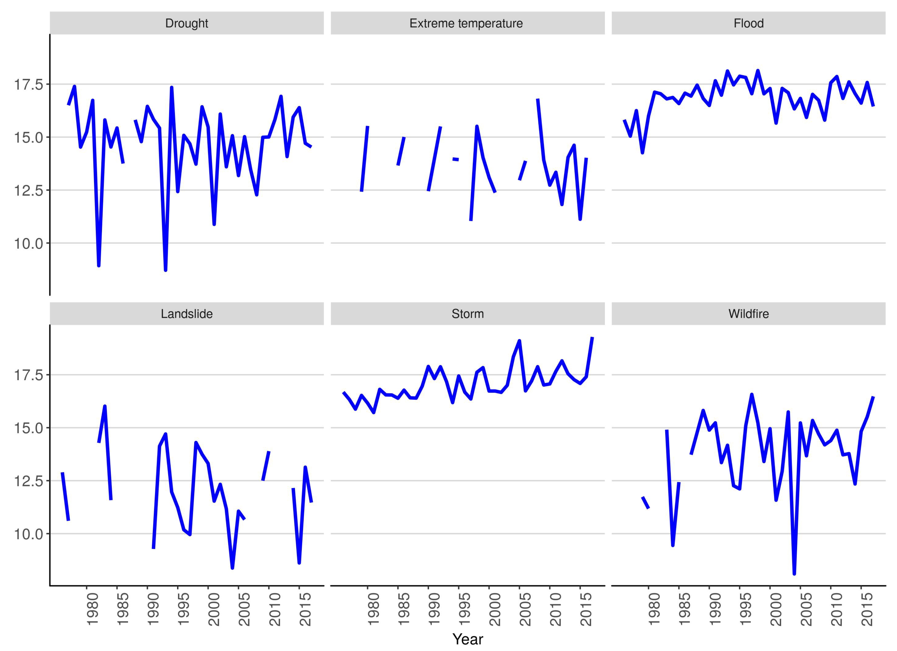
Figure A1 depicts results on the logarithm of real—deflated by the GDP deflator—estimated damages between 1976 and 2017. Due to a lack of data we are not showing results by regions here, but worldwide aggregated data only. As can be seen from the Figure, data on real damages is hard to analyze because of many missing values. Indeed, for some disaster categories real damages are missing for certain years.
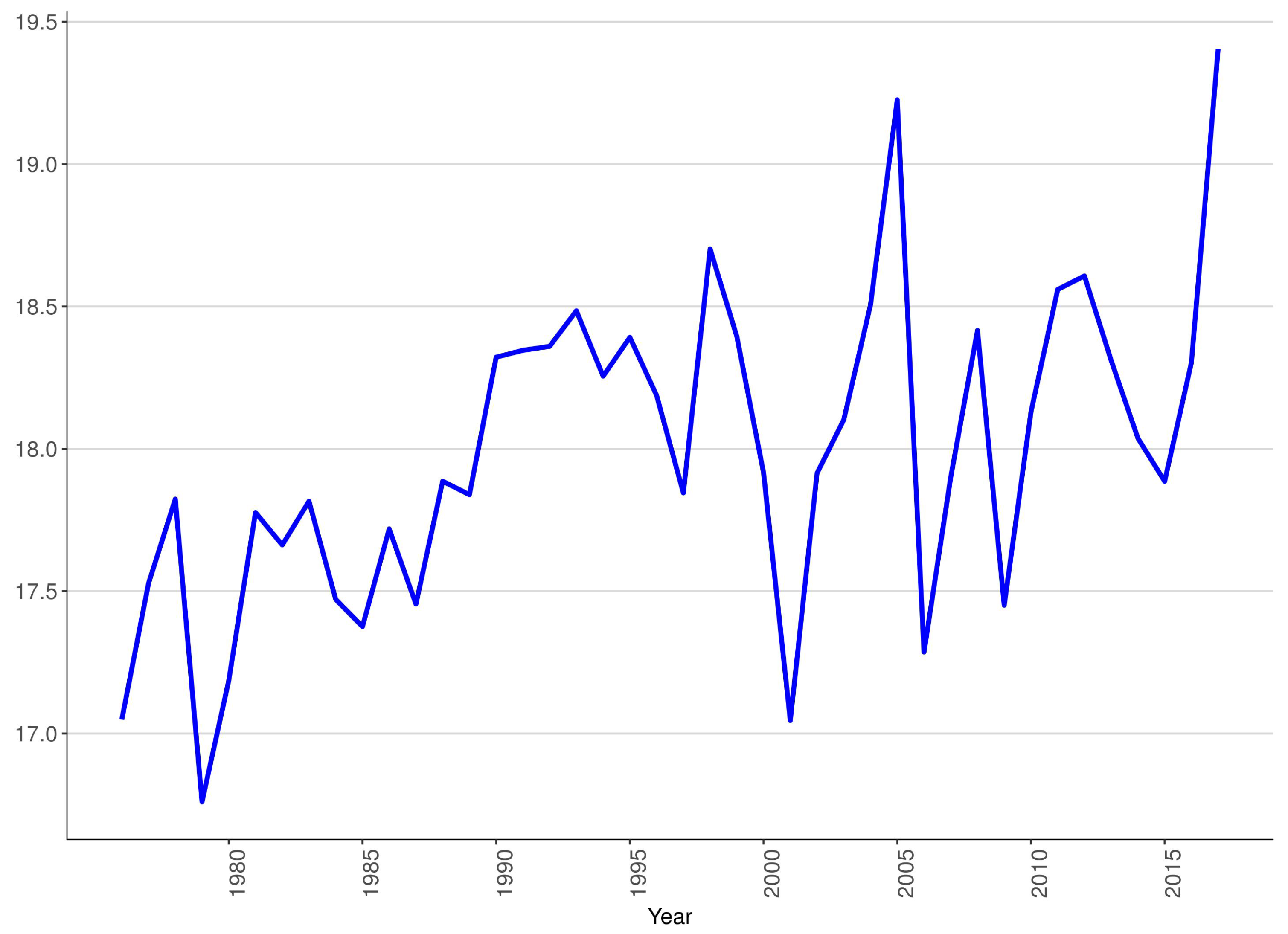
Data shown in Figure A1 is summed up and plotted in Figure A2 as total estimated damage. Figure A1 shows that real damage costs increased for the disaster category storm in recent years. Fluctuations in storm related damages also dominate aggregated damage costs (Figure A2). Thus, given the severe data issues at hand, we focus on the number of disasters per year instead of disaster cost in our empirical analysis. Furthermore, societal changes, such as population and wealth increases, and exceptionally big disasters, e.g. Hurricane Sandy, may distort damage costs. In fact, Mohleji and Pielke (2014) argue that societal changes are sufficient to explain increasing disaster damages; see also Bouwer (2011).
Figure A1.
Logarithm of estimated real damages for climate related disaster between 1976 and 2017 by disaster category.
Figure A1.
Logarithm of estimated real damages for climate related disaster between 1976 and 2017 by disaster category.

Figure A2.
Logarithm of estimated real damages for climate disaster between 1976 and 2017; total.

References
- Adam, Christopher S, and David Bevan. 2014. Public Investment, Public Finance, and Growth; The Impact of Distortionary Taxation, Recurrent Costs, and Incomplete Appropriability. IMF Working Papers 14/73. Washington, DC: International Monetary Fund. [Google Scholar]
- Azariadis, Costas, and John Stachurski. 2005. Poverty traps. In Handbook of Economic Growth, 1st ed. Edited by Philippe Aghion and Steven Durlauf. Amsterdam: Elsevier, vol. 1, Part A, Chapter 05. [Google Scholar]
- Banga, Josue. 2018. The green bond market: A potential source of climate finance for developing countries. Journal of Sustainable Finance & Investment 18: 1–16. [Google Scholar] [CrossRef]
- Barro, Robert J. 2006. Rare disasters and asset markets in the twentieth century. The Quarterly Journal of Economics 121: 823–66. [Google Scholar] [CrossRef]
- Barro, Robert J., and Jose F. Ursua. 2008. Macroeconomic Crises Since 1870. Working Paper 13940. Cambridge: National Bureau of Economic Research. [Google Scholar] [CrossRef]
- Batten, Sandra. 2018. Climate Change and the Macro-Economy: A Critical Review. Bank of England Working Papers No. 706. Bank of England: London. [Google Scholar]
- Battiston, Stefano, Antoine Monasterolo Mandel, Franziska Schuetze, and Gabriele Visentin. 2017. A climate stress-test of the financial system. Nature Climate Change 7: 283–88. [Google Scholar] [CrossRef]
- Bernard, Lucas, and Willi Semmler. 2015. The Oxford Handbook of the Macroeconomics of Global Warming. OUP Catalogue. Oxford: Oxford University Press. [Google Scholar]
- Bevan, David, and Christopher Adam. 2016. Financing the Reconstruction of Public Capital after a Natural Disaster. Policy Research Working Paper 7718. Washington, DC: World Bank. [Google Scholar]
- Bonen, Anthony, Prakash Loungani, Willi Semmler, and Sebastian Koch. 2016. Investing to Mitigate and Adapt to Climate Change: A Framework Model. Working Paper 16/164. Washington, DC: International Monetary Fund. [Google Scholar]
- Bouwer, Laurens M. 2011. Have disaster losses increased due to anthropogenic climate change? Bulletin of the American Meteorological Society 92: 39–46. [Google Scholar] [CrossRef] [Green Version]
- Burke, Marshall, Solomon M. Hsiang, and Edward Miguel. 2015. Global non-linear effect of temperature on economic production. Nature 527: 235–39. [Google Scholar] [CrossRef]
- Cantelmo, Alessandro, Giovanni Melina, and Chris Papageorgiou. 2017. Climate Change and Macroeconomic Outcomes in Low-Income Countries. Technical Report. Washington, DC: IMF. [Google Scholar]
- Catalano, Michele, Lorenzo Forni, and Emilia Pezzolla. 2018. Climate-Change Adaptation: The Role of Fiscal Policy. Technical Report. Cesena: University of Bologna. [Google Scholar]
- Cohen, Gail, Joao Tovar Jalles, Prakash Loungani, and Ricardo Marto. 2018. The long-run decoupling of emissions and output: Evidence from the largest emitters. Energy Policy 118: 58–68. [Google Scholar] [CrossRef]
- Coronese, Matteo, Francesco Lamperti, Francesca Chiaromonte, and Andrea Roventini. 2018. Natural Disaster Risk and the Distributional Dynamics of Damages. LEM Working Paper Series 2018/22. Pisa: Laboratory of Economics and Management (LEM), Sant’Anna School of Advanced Studies. [Google Scholar]
- Crépin, Anne-Sophie, and Eric Nævdal. 2019. Inertia risk: Improving economic models of catastrophes. The Scandinavian Journal of Economics. forthcoming. [Google Scholar] [CrossRef]
- Dell, Melissa, Benjamin F. Jones, and Benjamin A. Olken. 2012. Temperature shocks and economic growth: Evidence from the last half century. American Economic Journal: Macroeconomics 4: 66–95. [Google Scholar] [CrossRef] [Green Version]
- Elliott, Graham, Thomas J. Rothenberg, and James H. Stock. 1996. Efficient Tests for an Autoregressive Unit Root. Econometrica 64: 813–36. [Google Scholar] [CrossRef] [Green Version]
- Engle, Robert F., and Clive W. J. Granger. 1987. Co-integration and error correction: Representation, estimation, and testing. Econometrica 55: 251–76. [Google Scholar] [CrossRef]
- Faulwasser, Timm, Marco Gross, Willi Semmler, and Prakash Loungani. 2020. Uncoventional monetary policy in a nonlinear quadratic model. Studies in Nonlinear Dynamics and Econometrics. forthcoming. [Google Scholar]
- Fernandez-Villaverde, Jesus, and Oren Levintal. 2016. Solution Methods for Models with Rare Disasters. Working Paper 21997. Cambridge: National Bureau of Economic Research. [Google Scholar] [CrossRef]
- Flaherty, Michael, Arkady Gevorkyan, Siavash Radpour, and Willi Semmler. 2017. Financing climate policies through climate bonds—A three stage model and empirics. Research in International Business and Finance 42: 468–79. [Google Scholar] [CrossRef]
- Fratzscher, Marcel, Christoph Grosse Steffen, and Malte Rieth. 2017. Inflation Targeting as a Shock Absorber. Working Papers 655. Paris: Banque de France. [Google Scholar]
- Gabaix, Xavier. 2011. Disasterization: A simple way to fix the asset pricing properties of macroeconomic models. The American Economic Review 101: 406–9. [Google Scholar] [CrossRef]
- Gallic, Ewen, and Gauthier Vermandel. 2020. Weather shocks. European Economic Review 124: 103409. [Google Scholar] [CrossRef]
- Gevorkyan, Aleksandr V. 2008. Fiscal policy and alternative sources of public capital in transition economies: The diaspora bond. Journal of International Business and Economy 9: 33–61. [Google Scholar]
- Gevorkyan, Arkady, Michael Flaherty, Dirk Heine, Mariana Mazzucato, Siavash Radpour, and Willi Semmler. 2016. Financing Climate Policies through Carbon Taxation and Climate Bonds—Theory and Empirics. Technical Report. New York: The New School for Social Research. [Google Scholar]
- Gourio, Francois. 2012. Disaster risk and business cycles. American Economic Review 102: 2734–66. [Google Scholar] [CrossRef] [Green Version]
- Greiner, Alfred, Lars Gruene, and Willi Semmler. 2010. Growth and climate change: Threshold and multiple equilibria. In Dynamic Systems, Economic Growth, and the Environment. Edited by Jesús Crespo Cuaresma, Tapio Palokangas and Alexander Tarasyev. Volume 12 of Dynamic Modeling and Econometrics in Economics and Finance. Berlin and Heidelberg: Springer, pp. 63–78. [Google Scholar]
- Gross, Marco, Prakash Loungani, and Willi Semmler. 2019. Unconventional Monetary Policy in a Nonlinear Quadratic Model. Working Paper. New York: The New School. [Google Scholar]
- Guha-Sapir, Debarati, Indhira Santos, and Alexandre Borde. 2013. The Economic Impacts of Natural Disasters. Oxford: Oxford University Press. [Google Scholar]
- Gumbel, Emil Julius. 1958. Statistics of Extremes. New York: Columbia University Press. [Google Scholar]
- Hotelling, Harold. 1931. The economics of exhaustible resources. Journal of Political Economy 39: 137–75. [Google Scholar] [CrossRef]
- IMF. 2017. World Economic Outlook, October 2017: Seeking Sustainable Growth: Short-Term Recovery, Long-Term Challenges. World Economic Outlook. Washington, DC: International Monetary Fund. [Google Scholar]
- Ingham, Alan, Jie Ma, and Alistair Ulph. 2007. Climate change, mitigation and adaptation with uncertainty and learning. Energy Policy 35: 5354–69. [Google Scholar] [CrossRef]
- IPCC. 2012. Managing the Risks of Extreme Events and Disasters to Advance Climate Change Adaptation. A Special Report of the Intergovernmental Panel on Climate Change. Technical Report. Cambridge: Intergovernmental Panel on Climate Change. [Google Scholar]
- IPCC. 2013. Summary for policymakers. In The Physical Science Basis. Contribution of Working Group 1 to the Fifth Assessment Report of the Intergovernmental Panel of Climate Change. Fifth Assessment Report. Cambridge: Cambridge University Press. [Google Scholar]
- Kovacevic, Raimund M., and Georg Ch. Pflug. 2011. Does insurance help to escape the poverty trap?—A ruin theoretic approach. Journal of Risk and Insurance 78: 1003–28. [Google Scholar] [CrossRef]
- Kovacevic, Raimund M., and Willi Semmler. 2020. Poverty traps and disaster insurance in a bi-level decision framework. In Dynamic Economic Problems with Regime Switches. Dynamic Modeling and Econometrics in Economics and Finance. Edited by Vladimir M. Veliov, Josef L. Haunschmied, Raimund Kovacevic and Willi Semmler. Berlin and Heidelberg: Springer. [Google Scholar]
- Kwiatkowski, Denis, Peter Phillips, Peter Schmidt, and Yongcheol Shin. 1992. Testing the null hypothesis of stationarity against the alternative of a unit root: How sure are we that economic time series have a unit root? Journal of Econometrics 54: 159–78. [Google Scholar] [CrossRef]
- Lean, Judith L., and David H. Rind. 2008. How natural and anthropogenic influences alter global and regional surface temperatures: 1889 to 2006. Geophysical Research Letters 35. [Google Scholar] [CrossRef] [Green Version]
- Letta, Marco, and Richard S. J. Tol. 2019. Weather, Climate and Total Factor Productivity. Environmental & Resource Economics 73: 283–305. [Google Scholar] [CrossRef] [Green Version]
- Marto, Ricardo, Chris Papageorgiou, and Vladimir Klyuev. 2017. Building Resilience to Natural Disasters: An Application to Small Developing States. IMF Working Paper 17/223. Washington, DC: International Monetary Fund. [Google Scholar]
- Maurer, Helmut, and Willi Semmler. 2011. A model of oil discovery and extraction. Applied Mathematics and Computation 217: 1163–69. [Google Scholar] [CrossRef]
- McKibbin, Warwick J., Adele C. Morris, Augustus Panton, and Peter Wilcoxen. 2017. Climate Change and Monetary Policy: Dealing with Disruption. CAMA Working Paper 77/2017. Canberra: Centre for Applied Macroeconomic Analysis. [Google Scholar]
- Miller, Ron L., Gavin A. Schmidt, Larissa S. Nazarenko, Nick Tausnev, Susanne E. Bauer, Anthony D. DelGenio, Max Kelley, Ken K. Lo, Reto Ruedy, Drew T. Shindell, and et al. 2014. Cmip5 historical simulations (1850–2012) with giss modele2. Journal of Advances in Modeling Earth Systems 6: 441–78. [Google Scholar] [CrossRef]
- Mohleji, Shalini, and Roger Pielke. 2014. Reconciliation of trends in global and regional economic losses from weather events: 1980-2008. Natural Hazards Review 15: 04014009. [Google Scholar] [CrossRef] [Green Version]
- Monnin, Pierre. 2018. Central Banks and the Transition to a Low-Carbon Economy. Working Paper 2018/1. Zurich: Council on Economic Policies. [Google Scholar]
- NASEM. 2016. Attribution of Extrem Weather Events in the Context of Climate Changes. Washington, DC: The National Academies Press. [Google Scholar] [CrossRef] [Green Version]
- Pindyck, Robert. 1978. The optimal exploration and production of nonrenewable resources. Journal of Political Economy 86: 841–61. [Google Scholar] [CrossRef]
- Rietz, Thomas A. 1988. The equity risk premium a solution. Journal of Monetary Economics 22: 117–31. [Google Scholar] [CrossRef]
- Semmler, Willi, and Marvin Ofori. 2007. On poverty traps, thresholds and take-offs. Structural Change and Economic Dynamics 18: 1–26. [Google Scholar] [CrossRef]
- Semmler, Willi, Helmut Maurer, and Anthony Bonen. 2018a. Control Systems and Mathematical Methods in Economics. Lecture Notes in Economics and Mathematical Systems. Chapter An Extended Integrated Assessment Model for Mitigation and Adaptation Policies on Climate Change. Berlin: Springer, vol. 687, pp. 297–317. [Google Scholar]
- Semmler, Willi, Helmut Maurer, and Anthony Bonen. 2018b. Financing Climate Change Policies: A Multi-Phase Integrated Assessment Model for Mitigation and Adaptation. Working paper. New York: The New School. [Google Scholar]
- Stott, Peter. 2016. How climate change affects extreme weather events. Science 352: 1517–18. [Google Scholar] [CrossRef]
- Stott, Peter A., Nikolaos Christidis, Friederike E. L. Otto, Ying Sun, Jean-Paul Vanderlinden, Geert Jan van Oldenborgh, Robert Vautard, Hans von Storch, Peter Walton, Pascal Yiou, and et al. 2016. Attribution of extreme weather and climate-related events. WIREs Climate Change 7: 23–41. [Google Scholar] [CrossRef]
- Thomas, Vinod, and Ramon Lopez. 2015. Global Increase in Climate-Related Disasters. Working Paper 466. Manila: Asian Development Bank. [Google Scholar]
- Thomas, Vinod, Jose Ramon Albert, and Rosa Perez. 2013. Climate-Related Disasters in Asia and the Pacific. ADB Economic Working Paper 358. Manila: Asian Development Bank. [Google Scholar]
- UNCTAD. 2018. The Least Developed Countries Report 2017. New York: United Nations Conference on Trade and Development. [Google Scholar] [CrossRef]
- Weitzman, Martin L. 2009. Additive damages, fat-tailed climate dynamics, and uncertain discounting. Economics 3: 1–22. [Google Scholar]
- Zivot, Eric, and Donald W. K Andrews. 2002. Further evidence on the great crash, the oil-price shock, and the unit-root hypothesis. Journal of Business & Economic Statistics 20: 25–44. [Google Scholar] [CrossRef]
| 1 | |
| 2 | From an empirical point of view the evidence on persistently low growth after a disaster shock is strong, especially for lower-income countries, but not unambiguous. Some studies argue that due to “creative destruction” a strong recovery after the disaster shock may take place. However, most studies find a negative long-run effect. See Batten (2018) for a detailed overview. |
| 3 | https://www.emdat.be/; EMDAT reports events which cause at least 10 deaths, affect at least 100 people, or prompt a declaration of a state of emergency or a call for international assistance as a disaster. |
| 4 | Data on real climate disaster cost is provided in Appendix A.2. Figure A1 and Figure A2 show severe data issues for climate disaster cost. We regard the number of climate-related disasters as the more reliable indicator and therefore focus on it in this section. |
| 5 | In our empirical analysis we focus on the seven regions identified by the World Bank Atlas method: https://datahelpdesk.worldbank.org/knowledgebase/articles/906519-world-bank-country-and-lending-groups |
| 6 | See https://www.esrl.noaa.gov/gmd/ccgg/trends/gr.html for more details on the data. |
| 7 | Thomas and Lopez (2015) include average temperature deviations as a regressor in explaining the frequency of intense climatological disasters and do not find any significant effect. Atmospheric CO2 levels, on the other hand, are significant in their analysis. Similarly, Letta and Tol (2019) only find evidence of a negative effect of temperature increases on TFP for “poor” countries. |
| 8 | See again https://www.esrl.noaa.gov/gmd/ccgg/trends/gr.html for more details. Regression results are not affected by altering the lag length for variable Sum of CO2 increases. |
| 9 | Similar results were obtained in a GLM panel model based on a Poisson and a negative binomial model. The results are not reported here. |
| 10 | Results on the fixed-effects coefficients can be found in the Appendix A. |
| 11 | For a further description of this model and its analytical treatment see Bonen et al. (2016) |
| 12 | Here the multi-factor productivity A is taken as constant but it could be made time-varying to capture the slow productivity decline resulting from slow temperature increases. |
| 13 | |
| 14 | In more recent stochastic models with trapping probabilities such a regime is also referred to as a trapping region (Kovacevic and Pflug 2011), see also Kovacevic and Semmler (2020). For modeling endogenous catastrophic risk see Crépin and Nævdal (2019). |
| 15 | For details see Kovacevic and Semmler (2020). |
| 16 | We do not model the resulting temperature effects directly since changes in temperature, as well as in precipitation levels, are mainly due to GHG emission as discussed in Section 2. Therefore we are focusing on CO2 emission as the most significant man-made GHG. |
| 17 | One might think of passing beyond a tipping point in climate change, as in Greiner et al. (2010), where a sequence of disasters is likely to occur. |
| 18 | Note that given the quality and heterogeneity of the data it is very hard to undertake more precise parameter calibration. We therefore do some robustness tests with different parameter constellations. The robustness tests are undertaken for different parameter values concerning the dynamic state equations for the occurring disaster phase of the model. |
| 19 | A model version with time-varying switching points can be found in Semmler et al. (2018b). |
| 20 | Note that we could define a sequence of highly correlated disaster shocks, as it is done in Catalano et al. (2018), which gives roughly the same results. |
| 21 | |
| 22 | We want to thank Arkady Gevorkyan for providing us with the data for Figure 8. |
| 23 | We want to note that after the 2007–2009 meltdown a lot of literature has been generated on the prevention and mitigation of financial disasters through financial market regulation, such as regulation on requirements for required capital buffers for banks, system risk supervision, restriction of proprietary trading, policies on to big to fail, etc. Monetary and financial policies have been developed to prevent and to adapt when vulnerabilities and financial disasters risks occur. Monetary policy has moved from conventional to unconventional monetary policy with large asset purchasing programs, in particular, bond purchasing programs; see Faulwasser et al. (2020) and also Gross et al. (2019). |
| 24 | There is literature that views credit flows as a major driver for expansions and contractions. For a survey see Faulwasser et al. (2020). |
| 25 | |
| 26 | This would mean avoiding trapping probabilities as discussed in Kovacevic and Pflug (2011). |
Figure 1.
Frequency of climate related disaster (total) between 1976 and 2017 by region. Regional classification follows the World Bank classification system. Source: Authors’ estimates based on data from EMDAT.
Figure 1.
Frequency of climate related disaster (total) between 1976 and 2017 by region. Regional classification follows the World Bank classification system. Source: Authors’ estimates based on data from EMDAT.

Figure 2.
Annual CO2 mole fraction increase (in parts per million) from 1976 until 2017. The data is provided by the Mauna Loa Observatory.
Figure 2.
Annual CO2 mole fraction increase (in parts per million) from 1976 until 2017. The data is provided by the Mauna Loa Observatory.

Figure 3.
Government debt in a three-phase model, red: weak shock, blue: strong shock.

Figure 4.
Government capital in a three-phase model, red: weak shock, blue: strong shock.

Figure 5.
Private capital stock in a three-phase model; red: weak shock, blue: strong shock.

Figure 6.
Fossil fuel consumption in a three-stage model, red: weak shock, blue: strong shock.

Figure 7.
Path of consumption in a three-stage model; red: weak shock, blue: strong shock.

Figure 8.
Carbon Tax Policy and Issuance of Climate Bounds. The left-hand scale measures the proportion of global GHG emissions covered by carbon tax policy. The green bars represent their values over time. The right-hand scale measures the amount of climate bonds issued in USD (in millions). The blue line represents its value over time. Amount of climate bonds issued is reported only up until 03/20/2019. The number of issued bonds for 2019 is interpolated for the remaining 9 months. No data is available for the years 1993–1995, 1997–1999, 2001–2003 and 2005–2006. Source: Climate Bond Initiative, World Bank.

Table 1.
Stationarity test for Disaster Frequency for East Asia and Pacific (EAS), Europe and Central Asia (ECS), Latin America and the Caribbean (LCN), Middle East and North Africa (MEA), North America (NAC), South Asia (SAS), and Sub-Saharan Africa (SSF) and CO2 level. KPSS Test: test by Kwiatkowski et al. (1992) with trend and two lags. ADF Test Trend: augmented Dickey–Fuller test with trend and two lags. ADF Test Drift: augmented Dickey–Fuller test with drift and two lags. ADF Test: augmented Dickey–Fuller test with two lags. DF-GLS Trend: DF-GLS test with trend and two lags. DF-GLS Constant: DF-GLS test with constant and two lags. ZA Test: Zivot and Andrews (2002) Unit Root Test with intercept and trend and two lags. ZA Test Trend: Zivot and Andrews (2002) Unit Root Test with trend and two lags. ZA Test Constant: Zivot and Andrews (2002) Unit Root Test with constant and two lags.
| Region | KPSS Test Statistic | ADF Test Trend | ADF Test Drift | ADF Test | DF-GLS Trend | DF-GLS Constant | ZA Test | ZA Test Trend | ZA Test Constant |
|---|---|---|---|---|---|---|---|---|---|
| EAS | ** | ||||||||
| ECS | ** | ** | |||||||
| MEA | ** | ||||||||
| LCN | ** | ||||||||
| NAC | *** | ** | ** | ||||||
| SAS | * | *** | * | * | |||||
| SSF | * | ||||||||
| CO2 | *** |
***, **, *.
Table 2.
Engle and Granger (1987) cointegration test with 2 lags for East Asia and Pacific (EAS), Europe and Central Asia (ECS), Latin America and the Caribbean (LCN), Middle East and North Africa (MEA), North America (NAC), South Asia (SAS), and Sub-Saharan Africa (SSF)
Table 2.
Engle and Granger (1987) cointegration test with 2 lags for East Asia and Pacific (EAS), Europe and Central Asia (ECS), Latin America and the Caribbean (LCN), Middle East and North Africa (MEA), North America (NAC), South Asia (SAS), and Sub-Saharan Africa (SSF)
| Region | Test Statistic |
|---|---|
| EAS | *** |
| ECS | ** |
| MEA | ** |
| LCN | *** |
| NAC | |
| SAS | *** |
| SSF |
***, **, *.
Table 3.
Fixed-effects Panel with clustered standard errors on the group level and small sample size correction. The dependent variable represents the number of disaster events for a given year (Disaster Frequency). Independent variables include the lagged value of the dependent variable (Disaster Frequency1) and the sum of the current and 17 most recent increases in CO2 concentration in the atmosphere, expressed as a mole fraction in dry air (ppm) (Sum of CO2 increases). Standard errors are given in parenthesis. Column Data Set considers all disasters in the EMDAT database. Column Large Disasters only includes disasters with at least 1000 affected or 100 people killed.
| Dependent Variable: | ||
|---|---|---|
| Disaster Frequency | ||
| Complete Data-Set | Large Disaster Data-Set | |
| Disaster Frequency1 | 0.517 *** | 0.618 *** |
| (0.113) | (0.077) | |
| Sum of CO2 increases | 0.947 *** | 0.626 *** |
| (0.300) | (0.181) | |
| Observations | 280 | 277 |
| R | 0.526 | 0.624 |
| Adjusted R | 0.512 | 0.612 |
| F Statistic | 150.216 *** (df = 2; 271) | 222.036 *** (df = 2; 268) |
*p < 0.1, **p < 0.05, ***p < 0.01.
Table 4.
Fixed-effects Panel with clustered standard errors on the group level and small sample size correction. The dependent variable represents the first difference of the number of disaster events for a given year (Diff Disaster Frequency). Independent variables include the lagged value of the dependent variable (Disaster Frequency1) and the sum of the current and 17 most recent increases in CO2 concentration in the atmosphere, expressed as a mole fraction in dry air (ppm) (Sum of CO2 increases). Standard errors are given in parenthesis. Column Data Set considers all disasters in the EMDAT database. Column Large Disasters only includes disasters with at least 1000 affected or 100 people killed.
| Dependent Variable: | ||
|---|---|---|
| Δ Disaster Frequency | ||
| Complete Data-Set | Large Disaster Data-Set | |
| Disaster Frequency1 | −0.483 *** | −0.382 *** |
| (0.113) | (0.077) | |
| Sum of CO2 increases | 0.947 *** | 0.627 *** |
| (0.300) | (0.181) | |
| Observations | 279 | 276 |
| R | 0.242 | 0.190 |
| Adjusted R | 0.219 | 0.166 |
| F Statistic | 43.215 *** (df = 2; 271) | 31.395 *** (df = 2; 268) |
*p < 0.1, **p < 0.05, ***p < 0.01.
Table 5.
Parameters defining weak and strong shocks for the three time periods.
| Time Period: | – | – | – |
| risk rate, weak shock | = 0.05 | ||
| risk rate, strong shock | = 0.10 | ||
| weak shock: , | 0.1, (0.075) | 0.12, (0.12) | 0.1, (0.075) |
| strong shock: , ) | 0.1, (0.075) | 0.17, (0.17) | 0.1, (0.075) |
© 2020 by the authors. Licensee MDPI, Basel, Switzerland. This article is an open access article distributed under the terms and conditions of the Creative Commons Attribution (CC BY) license (http://creativecommons.org/licenses/by/4.0/).
Share and Cite
MDPI and ACS Style
Mittnik, S.; Semmler, W.; Haider, A. Climate Disaster Risks—Empirics and a Multi-Phase Dynamic Model. Econometrics 2020, 8, 33. https://0-doi-org.brum.beds.ac.uk/10.3390/econometrics8030033
AMA Style
Mittnik S, Semmler W, Haider A. Climate Disaster Risks—Empirics and a Multi-Phase Dynamic Model. Econometrics. 2020; 8(3):33. https://0-doi-org.brum.beds.ac.uk/10.3390/econometrics8030033
Chicago/Turabian StyleMittnik, Stefan, Willi Semmler, and Alexander Haider. 2020. "Climate Disaster Risks—Empirics and a Multi-Phase Dynamic Model" Econometrics 8, no. 3: 33. https://0-doi-org.brum.beds.ac.uk/10.3390/econometrics8030033
Note that from the first issue of 2016, this journal uses article numbers instead of page numbers. See further details here.