Data Revisions and the Statistical Relation of Global Mean Sea Level and Surface Temperature


1
CREATES, Department of Economics and Business Economics, Aarhus University, 8000 Aarhus, Denmark
2
Department of Economics, University of Copenhagen, 1353 Copenhagen K, Denmark
3
Danish Metorological Institute, 2100 Copenhagen, Denmark
*
Authors to whom correspondence should be addressed.
Econometrics 2020, 8(4), 41; https://0-doi-org.brum.beds.ac.uk/10.3390/econometrics8040041
Submission received: 28 November 2018
/
Revised: 16 October 2020
/
Accepted: 21 October 2020
/
Published: 2 November 2020
(This article belongs to the Special Issue Celebrated Econometricians: David Hendry)
Abstract
:We study the stability of estimated linear statistical relations of global mean temperature and global mean sea level with regard to data revisions. Using four different model specifications proposed in the literature, we compare coefficient estimates and long-term sea level projections using two different vintages of each of the annual time series, covering the periods 1880–2001 and 1880–2013. We find that temperature and sea level updates and revisions have a substantial influence both on the magnitude of the estimated coefficients of influence (differences of up to 50%) and therefore on long-term projections of sea level rise following the RCP4.5 and RCP6 scenarios (differences of up to 40 cm by the year 2100). This shows that in order to replicate earlier results that informed the scientific discussion and motivated policy recommendations, it is crucial to have access to and to work with the data vintages used at the time.
1. Introduction
Historical time series of annual global surface temperature and global sea level are subject to frequent revisions. In this paper, we show that the statistical relation between the series estimated in semi-empirical models is sensitive to these revisions, and long-term projections derived using these coefficient estimates vary substantially across different “vintages” of data.
Global mean temperatures have increased since the industrial revolution as a consequence of CO and other greenhouse gas emissions mainly from combustion of fossil fuels, but also from land use and deforestation. This increase is measured in global mean temperature series that are compiled from a large set of station measurements with global coverage (Hansen et al. 2010; Morice et al. 2012; Vose et al. 2012).
Global sea level has increased since the late nineteenth century and is expected to rise further as a consequence of anthropogenic climate change with far-reaching ramifications and economic consequences (Desmet et al. 2020). The rise is caused by thermal expansion of the ocean (Zanna et al. 2019), by loss of mass of glaciers, by loss of mass from ice sheets (IPCC 2019), and by land water storage change (Chao et al. 2008). To understand past changes and to give scenarios for future changes, process-based modeling is applied, in which the different components of the climate system—the atmosphere-ocean, land, and cryosphere are modeled (Church et al. 2013; IPCC 2019). For a general discussion of global sea level change, see also (Gregory et al. 2013).
Semi-empirical models have been developing and applying to complement process-based modeling (see, for example, Jackson et al. (2018) for an application. Semi-empirical models aim at establishing statistical relationships between time series of the global sea level and associated time series of drivers, such as surface temperature. They are a pragmatic response to the current limitations of process-based models to project future sea level rise (Grinsted et al. 2010).
This motivates the statistical study of the relationship between global sea level and surface temperature. The global aggregated time series are subject to frequent revisions and improvements. Neither global mean temperature nor global mean sea level are directly observable, and the construction of indices to approximate these objects is therefore fraught with measurement error. The revisions reflect efforts to reduce this measurement error.
For completeness, we note that with the emergence of proxy-based reconstructions of sea level reaching back before the instrumental era, semi-empirical studies also have to be extended to cover a longer time span of some millennia, e.g., (Kopp et al. 2016).
In this paper, we are interested in the question to what extent these data revisions have an influence on the estimation of parameters in semi-empirical models. The econometric literature has considered the problem of measurement errors in different contexts. For the treatment of measurement errors in variables in regression models, see, for example, (Hendry 1995, chp. 12), in state-space models, see Durbin and Koopman (2012), and in cointegration analysis, see Duffy and Hendry (2017).
Our approach in this paper is to repeat the analyses in Grassi et al. (2013); Rahmstorf (2007); Schmith et al. (2012); Vermeer and Rahmstorf (2009), using different vintages of the time series for temperature and sea level that were employed in these studies. This approach mimics the situation of a researcher who tries to replicate the results of earlier studies with new vintages of the same data sets. Bolin et al. (2015); Rahmstorf et al. (2012) are closely related studies. We show that the estimated parameters that link temperature to changes in sea level, or the level itself in the case of cointegration analyses, are quite sensitive to data revisions. The long-term sea level projections based on scenario data for temperature also vary to a substantial extent in reaction to the changes in the parameter estimates.
The rest of the paper is organized as follows. In Section 2, we discuss the data set used in this paper. In Section 3, we estimate three models on the different configurations of old and new data and present future sea level projections from the different models and data configurations. In Section 4, we discuss the results and identify influential data points in the updates from the old to the new vintages that drive changes in the parameter estimates. Section 5 concludes.
2. Data and Revisions
Global surface temperature change time series are compiled by several groups, among them the NASA Goddard Institute for Space Studies (GISS), Hansen et al. (2010), the UK Meteorological Office Hadley Centre joint with the University of East Anglia Climatic Research Unit (HadCRUT), Morice et al. (2012),1 and the NOAA National Climatic Data Center, Vose et al. (2012).2 Global mean sea level time series are compiled by, for example, Church and White (2011); Hay et al. (2015); Ray and Douglas (2011).
In this study, we use the GISS global surface temperature change data set described by Hansen et al. (1981); Hansen and Lebedeff (1987); Hansen et al. (1999, 2001, 2010). The data are available from NASA (2020). 3 All data used in this paper are annually averaged series. Since our focus is on the influence of revisions, we consider different vintages of the global temperature time series, that is, versions of the series downloaded from the GISS web site at different times. The first vintage is the one used in Vermeer and Rahmstorf (2009) for the period 1880–2001, which we call . It was downloaded by the authors in July 2009. We compare this vintage to one, downloaded in October 2018, which covers the period 1880–2017. We denote this series where “year” states the endpoint of the sample period used in the statistical analysis. All temperature series are so-called temperature anomalies, i.e., differences from a 1951–1980 mean value.
The inputs to the GISS data set are quality-controlled surface temperature measurements from meteorological stations and ocean surface temperature measurements. Then, a gridding procedure is applied to produce a degree gridded data set, where each grid point value is influenced by stations up to 1200 km away, allowing nearly global coverage. Finally, global or regional averages can be produced from the gridded data set. Besides including updated observation records, the main difference between the two vintages is an altered procedure for either omitting or adjusting urban stations, to minimize spurious temperature changes due to urban effects.
For the sea level, we use the CSIRO sea level time series as described in Church and White (2006); Church et al. (2004) for the years 1880–2001, which we call . This is the first vintage. The second vintage is the revision4 described in Church and White (2011), which has been updated to 2013, which we call . Finally we use this new series restricted to the same period as the old series, 1880–2001, which we call . All sea level time series5 are so-called anomalies, i.e., differences from a 1989–1990 mean.
Sea level records reaching back 100 years or more are available from coastal tide gauge stations, island based tide gauges begin to appear from the 1950’s onwards, and therefore, the open ocean is unobserved over long periods. This implies challenges when estimating the global sea level and its changes, see Holgate et al. (2013). The CSIRO data set is constructed as a combination of tide-gauge data and satellite altimetry, which provides global coverage since 1992. Church and White (2011) discuss some of the differences in the two vintages, among them a larger set of locations. See Calafat et al. (2014) for an assessment of the methodology.
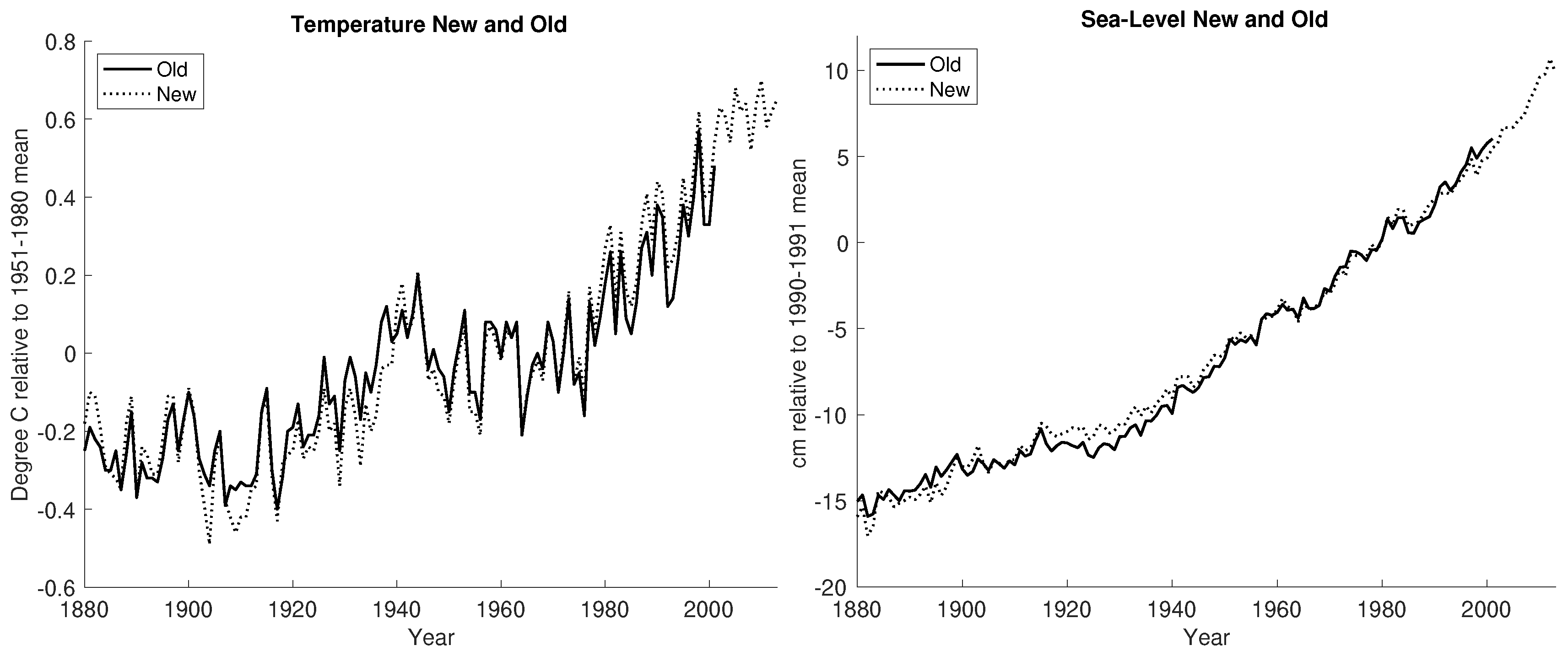
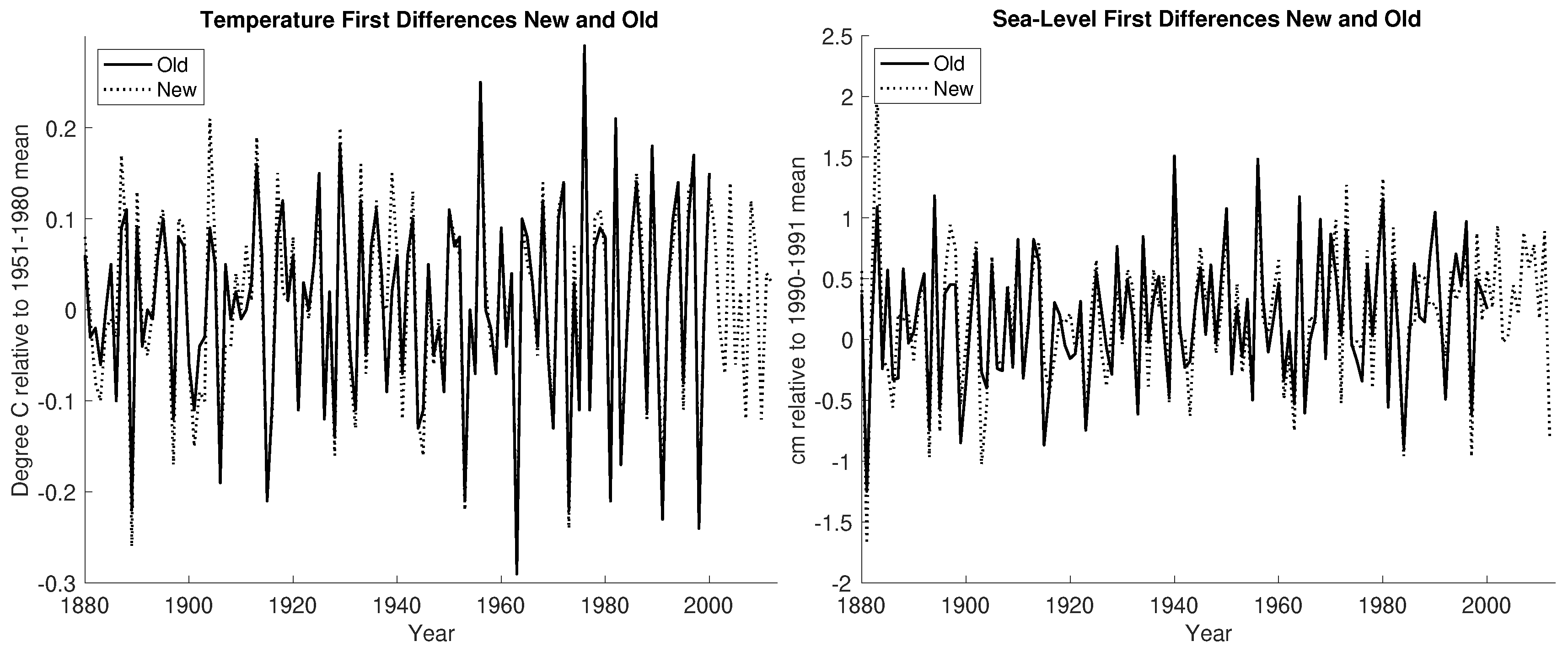
The left panel of Figure 1 shows the temperature time series of the 2001 vintage () and of the 2013 vintage restricted to 1880–2001 (). The right panel shows the two vintages of the sea level time series. Figure 2 shows first differences of the old and new vintages of sea level data.
We follow Church and White (2011); Vermeer and Rahmstorf (2009) and apply the reservoir correction proposed in Chao et al. (2008) to both old and new vintages.6 The left panel of Figure 3 shows the old vintage of the time series of the sea level with and without reservoir correction according to Chao et al. (2008) in the period 1880–2001. The right panel shows the same for the new vintage of sea level. The correction mainly has an influence on the latter part of the record after 1950.
We have also run our analysis on the data without reservoir correction, and while the findings are qualitatively similar, the numerical results differ. These results are available upon request. Using the correction facilitates comparability in particular to Vermeer and Rahmstorf (2009). Note that there are also estimates of the sea level contribution for the extraction from ground water to complement the terrestrial reservoir storage estimates (Wada et al. 2016).
3. The Effect of Revisions on Four Semi-Empirical Models
In this section, we repeat the analyses proposed in Grassi et al. (2013); Rahmstorf (2007); Schmith et al. (2012); Vermeer and Rahmstorf (2009) on five combinations of data and compare the results, using the series and for sea level and temperature, then , and finally for the longer period the series , in order to assess changes in the estimated parameters. We also analyze the models using the combinations , and , in order to assess whether changes in the estimated parameters are due to the updates in the sea level or the updates in temperature. The results are presented in Table 1, Table 2, Table 3, Table 4 and Table 5.
The studies in Grassi et al. (2013); Rahmstorf (2007); Vermeer and Rahmstorf (2009) relate first differences in sea level (Figure 2, right panel) to the level of temperature (Figure 1, left panel). The study in Schmith et al. (2012), on the other hand, relates sea level data (Figure 1, right panel) to temperature in levels (Figure 1, left panel) by including lagged sea level in the equation for and analysing a cointegrated vector autoregressive model for both temperature and sea level in the resulting error-correction model.
3.1. The Model Proposed by Rahmstorf
Rahmstorf (2007) proposed a linear regression model for sea level changes on temperature levels:
where denotes sea level anomaly relative to the 1989/90 mean, temperature, the 1951–1980 mean, and extracts a smooth component by singular spectrum analysis followed by 15-year binning (Moore et al. 2005).
Table 1 shows the estimated regression coefficients in a regression of on and a constant and their standard errors for the five combinations of data. The regression coefficient estimated on the revised data is , which is numerically 60 per cent of the size of the estimate from the old data, , which is . Note that the latter is not a replication of the result reported in Rahmstorf (2007), which was , because the vintage is the one used for Vermeer and Rahmstorf (2009), which is different from the one used in Rahmstorf (2007). Note also that the standard errors are calculated under standard assumptions on ordinary least squares, which we have critically discussed in Grassi et al. (2013); Schmith et al. (2007); Schmith et al. (2012). The 90%-confidence intervals based on the estimated variances do not overlap.
The other combinations give values in the interval to . In this case, the revision of the sea level time series has the largest influence on the estimation of the relation, since switching only the sea level series to the new vintage reduces the estimated coefficient from 0.26 to 0.43, whereas switching only the temperature series results in a reduction to 0.37. Our parameter estimation results are in alignment with earlier studies. Rahmstorf et al. (2012) focus on the sensitivity of semi-empirical models to different data sets for sea level and temperature. They also report results on the Rahmstorf (2007) model for the old and new vintage of the Church and White sea level data. They use the GISS and HadCRUT temperature time series, but they do not report when those data were downloaded, so we cannot know which vintage of the temperature series they employ. Nevertheless, in their Table 1, they report a regression coefficient of 0.45 for the old sea level data and GISS and a regression coefficient of 0.27 for the new sea level data and GISS. This is comparable to the estimates reported in the first line of our Table 1. In Bolin et al. (2015); Rahmstorf (2007) model is evaluated on the two vintages of Church and White sea level data and on two vintages of GISS temperature data, the one used in Rahmstorf (2007) and one downloaded for the purposes of writing Bolin et al. (2015). They report a regression coefficient of 0.44 for the old sea level vintage and the old temperature vintage and of 0.39 for the new temperature vintage, and they report a coefficient of 0.27 for the new sea level vintage paired with the old temperature vintage and of 0.27 for the new sea level vintage paired with the new temperature vintage (their -coefficient reported in their Table 2).
Semi-empirical sea level models were originally designed as a simple and pragmatic way of projecting global sea level into the future based on scenarios for global temperatures while “evading the unknowns pertaining to individual contributors” and to include behavior that is not captured in process-based models (Grinsted et al. 2010). In Rahmstorf (2007), projections based on the temperature scenarios from the IPCC 3rd assessment report were reported (IPCC 2001). The resulting sea level projections span the interval 55 to 91 cm by the year 2100.
For the purposes of this study, we are interested in the extent to which projections of this kind are sensitive to the data revisions and the entailed changes in the parameter estimates. We consider two temperature scenarios, the temperature trajectories of RCP4.5 and RCP6 (Masui et al. 2011; Meinshausen et al. 2011; Thomson et al. 2011) from 2002 until 2100. We use these trajectories as input to the estimated regression relations obtained from the five data configurations described above. For the samples ending in 2001, we project from the estimated equation
for and .
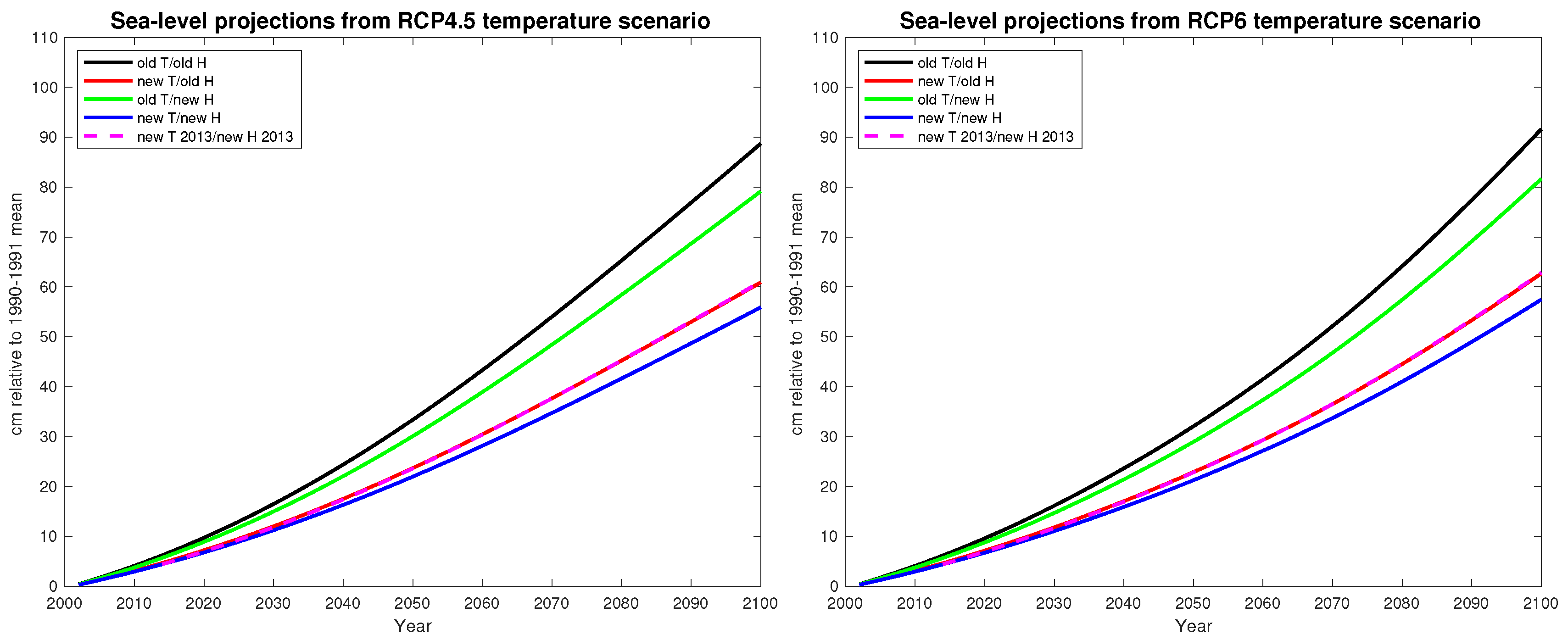
For the sample ending in 2013, we use and . Figure 4 shows the resulting sea level projections subtracting the initial level.
The projections show little difference between the scenarios, in line with similar results reported in (Church et al. 2013, Figure 13.10), which also show little difference in the 2100 projections for these two scenarios, even though the path and the longer term implications differ somewhat. The sea level increases by the year 2100 range between 55 and 92 cm. The old data set results in the highest projections and the new data set restricted until 2001 in the lowest. The new data set until 2013 results in a projection of 61 and 62 cm rise relative to the 1989/90 mean for the two RCP scenarios. This result is quite different from the one reported in Rahmstorf et al. (2012), who considered RCP4.5 and reported a range of the projection fan by the year 2100 of 20 cm for seven of nine of their data configurations.
3.2. The Model Proposed by Vermeer and Rahmstorf
Vermeer and Rahmstorf (2009) proposed an extension of the linear regression model in Rahmstorf (2007) to account for year-to-year changes in temperature:
where denotes sea level, temperature, the 1951–1980 temperature mean, and extracts a long-term trend by singular spectrum analysis followed by 15-year binning (Moore et al. 2005).
We report the results for the estimation of the regression (3) for configurations for old and new data in Table 2. It shows the estimated regression coefficients and their standard errors for the five possible combinations of data.
The regression coefficient estimated on the revised data is , which is numerically about 60 per cent of the size of the estimate from the old data, , which is . The results on the old data replicate those reported in Vermeer and Rahmstorf (2009). The 90%-confidence intervals based on the estimated variances do not overlap. The other combinations give values in the interval to . Again, the revision of the sea level time series has the largest influence on the estimation of the relation, since switching only the sea level series to the new vintage reduces the estimated coefficient from 0.55 to 0.34, whereas switching only the temperature series results in a reduction to 0.45. The results are in alignment with those reported in Rahmstorf et al. (2012), see their Table 1. There are also substantial differences in the estimate of b: Using new data on the 1880–2001 sample, the coefficient is reduced by 65% compared to the old data (from −4.94 to −1.73). It is also statistically insignificant on the new data. We also find that the revisions of the temperature time series have the largest influence, as evidenced by the results for the combinations and .
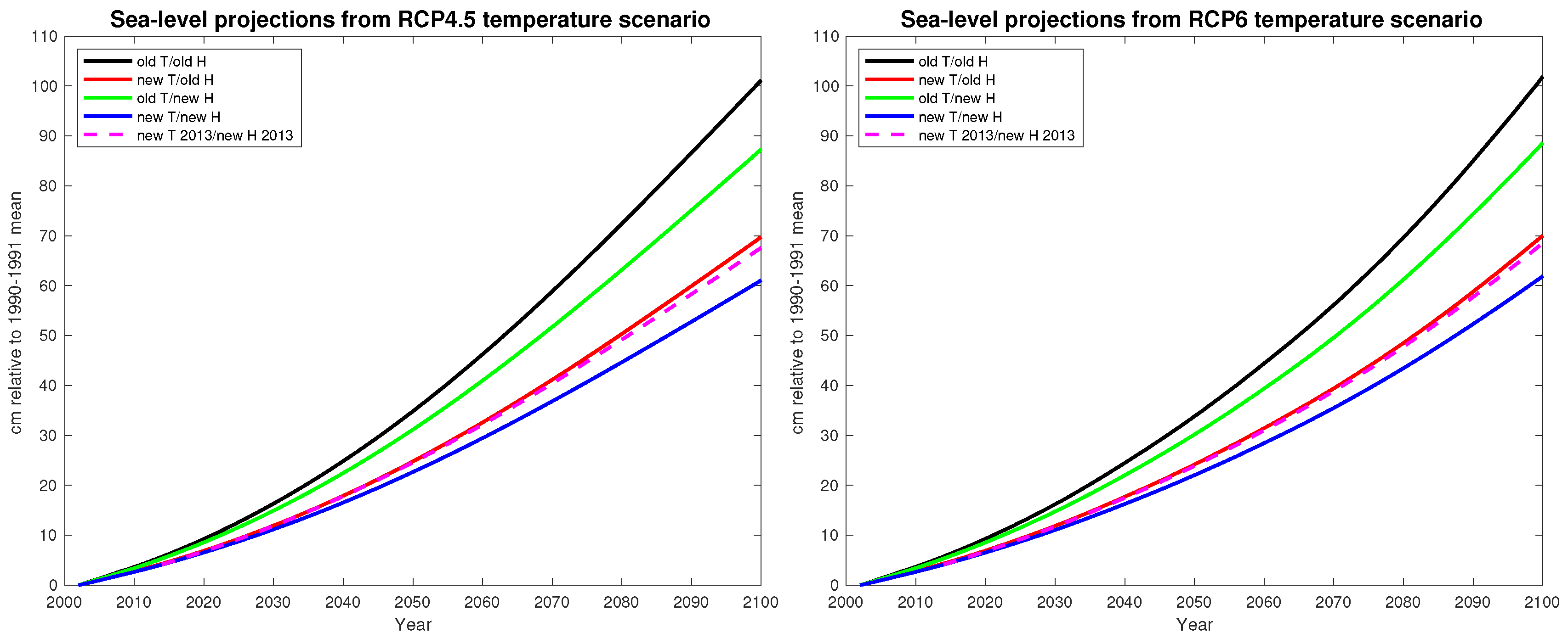
We repeat the sea level projection exercise using the RCP4.5 and RCP6 temperature scenarios. For the samples ending in 2001, we project using the equation
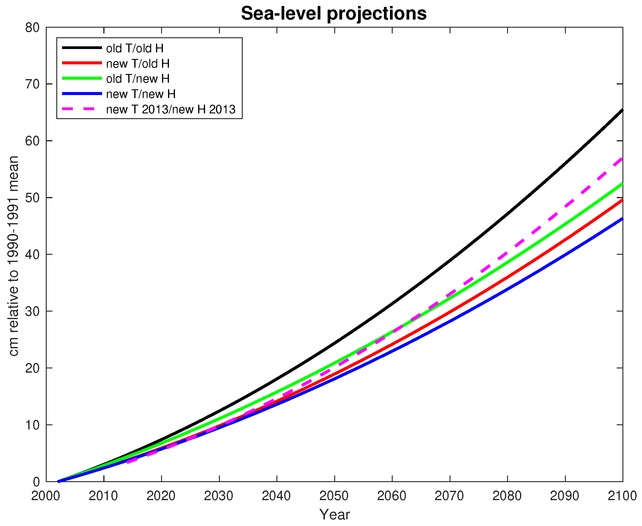
for and . For the sample ending in 2013, we use and accordingly, in both cases subtracting the first projected value. The results are shown in Figure 5. Again, the differences between RCP4.5 and RCP6 are minor. The sea level fan for RCP4.5 spans the interval from 61 to 101 cm by the year 2100, and similarly the sea level fan for RCP6 spans the interval from 62 to 102 cm, corresponding to 40 cm uncertainty due to data updates, given the two temperature scenarios. The old data set results in the highest projected sea level rises and the new data set until 2001 in the lowest. The new data set until 2013 results in 67 cm of sea level rise relative to the 1989/90 mean for both scenarios.
3.3. The Model Proposed by Grassi, Hillebrand and Ventosa-Santaulària
Grassi et al. (2013) formulate a state-space model that features a local linear trend model for each, sea level and temperature, and that linearly connects the trend in sea level with the one in temperature. They obtain a coefficient of influence of temperature on sea level changes that is comparable to the regression coefficient on the level of temperature in Vermeer and Rahmstorf (2009). The model specifies
where and are sea level and temperature with local linear trends and , respectively. Here the four processes are independent Gaussian i.i.d. processes. Note that and are variables, such that is whereas is This specification captures the idea of a linear relation of long-term trends in sea level differences and temperature levels. The equation for is essentially a regression of the variable on the variable with an error term . The model is estimated using the Kalman filter to maximize the Gaussian likelihood function. Inference in the model is conducted by simulation.
Table 3 shows the estimated coefficients of influence, , for the five possible data combinations. We provide confidence intervals for the estimated -coefficients by way of simulations. For each of the five combinations, we set a grid of data-generating values of , from −2 to 2 in steps of 0.20, setting the other parameters equal to the estimates from that data configuration. For each of the grid points, we set the data-generating equal to the grid point, simulate paths of the model, and estimate the model on each path without any constraints on . Then we find the 5th and 95th percentiles of the N estimates. We plot the upper and lower percentiles (y-axis) for each grid point (x-axis), resulting in 20 points for the lower percentile and 20 points for the upper percentile. It turns out that these points align on two almost straight lines. We find the data-estimate of on the y-axis of this plot, and read the confidence interval horizontally, by finding the x-values for which the two straight lines of the percentiles intersect with the constant data-estimate of on the y-axis. Thus, the intersection with the line that connects the upper percentiles yields the lower boundary of the confidence interval, and the intersection of the line that connects the lower percentiles yields the upper boundary of the confidence interval. The interpretation of this method is that the resulting confidence interval consists of the data-generating values of , for which the data-estimate of lies in the two-sided 90% acceptance region.
Similarly to Table 1 and Table 2, revisions in both the temperature and the sea level time series result in a decrease in the estimated coefficients on the period 1880–2001.
Also, updates to the temperature time series have about the same influence on the estimate as updates to the sea level time series. The estimation uncertainty in this model is estimated to be higher compared to the models of Schmith et al. (2012); Vermeer and Rahmstorf (2009). The confidence intervals for all configurations involving the old vintages include zero. When the new vintages are used on both sides of the equation, the confidence intervals do not contain zero. Note that the result on the configuration is not a replication of the one reported in Grassi et al. (2013), which was 0.46, since the data used in the original study is the same data set as the one used in Rahmstorf (2007). The “old” data set used here is the one from Vermeer and Rahmstorf (2009).
We also conduct a likelihood ratio test for constancy of the parameter with respect to the different vintages on the sample period 1880–2001. We specify a state-space model that contains two specifications of type (Section 3.3), one for and one for . We compare the log-likelihood value if we estimate the model unrestricted (resulting in two coefficients that are, essentially, and as in Table 3) with the log-likelihood value that results from imposing the restriction that the two coefficients are identical. The resulting likelihood-ratio statistic is equal to 0.057, implying a p-value from the chi-square distribution with one degree of freedom of , and so we cannot reject the null hypothesis that the two coefficients are the same, which supports the observation that the confidence intervals for both estimates contain the other estimate.
Finally, we project sea levels in Figure 6. Since the Grassi et al. (2013) model estimates a local trend specification for temperatures, we are not using RCP scenarios here, but we simulate data from the estimated temperature model, using as starting values the last value of the smoothed state variable from the estimated model. As data-generating parameters for the simulations, we use the estimated variances for and and the estimate for . We simulate from the model until we have 10,000 such processes for each of the five data configurations, with the corresponding sea level processes . The sea level scenarios in Figure 6 show, for each data configuration, the mean over those 10,000 processes for , where we subtract the smoothed state variable for last observation of .
The projections do not fan out as much as for the preceding models, resulting in a range of 19 cm difference by 2100. The basic pattern, however, is the same: The projection from the old data set is the highest, reaching 65 cm sea level rise over the 1989/90 mean. The projection from the new data set until 2001 is the lowest, at 46 cm sea level rise. The mixed data configurations are in between. The projection from the new data set through 2013 gives 57 cm sea level rise.
3.4. The Model Proposed by Schmith, Johansen and Thejll
Schmith et al. (2012) specify a vector autoregressive model for temperature, and sea level, In the analysis of and the Johansen (1996) cointegration test indicates that the variables cointegrate. The model can therefore be written in the vector error correction form
where and are adjustment coefficients that describe how the system is reacting to the stationary disequilibrium error
while and are nonstationary with stationary differences. The matrix has dimension and describes the short-run dynamics, and are linear drift terms, and is bivariate white noise. In the context of studying the link between sea level and temperature, the disequilibrium relation is of primary interest, because it describes how the non-stationary time series of temperature and sea level interact to form a stationary deviation , which is constant in equilibrium. Estimation is performed using Gaussian maximum likelihood and Table 4 shows the estimates of to be for the analysis of the period 1880–2013, using and .
These results are collected in Table 4. The analysis can be summarized by concluding that the results are not changed by using rather than , but changing the vintage of T has an effect on the coefficients. Based on the estimated variances, the implied 90%-confidence intervals of the coefficients estimated on and do not overlap, by a very small difference, but the 95% confidence intervals do overlap.
Table 5 reports the estimates for the adjustment coefficients and in Equation (11). The results for are highly significant, indicating an adjustment of temperature to the cointegrating relation, whereas the results for are insignificant, indicating that the sea level does not adjust to the cointegrating relation. This result is also obtained in Schmith et al. (2012), and it is discussed in detail there. Here we note that the significant estimates of do not vary much across the different data configurations, and thus the estimation of this coefficient does not appear very sensitive to the data revisions. The estimates of show more variation, but since they are all statistically indistinguishable from zero, the differences are not substantial either.
We do not report sea level projections for this model, since the physical mechanism discussed for the relation between sea level and temperature in Schmith et al. (2012) is opposite to that of the preceding models. Here, analysis of the adjustment coefficients from the cointegrating analysis suggests that surface temperature adjusts to changes in the ocean heat content, which is closely related to the sea level because of thermal expansion. In this conceptualization, it does not make sense to input a surface temperature into the model and to output a sea level “response”, as was done for the preceding models.
3.5. Summary
We have compared the analysis of three types of statistical time series models out of many possible models. Common to all of them is that we use a few (constant) parameters to describe the variation of the data, and the relation between the variables, and we investigate how these constants change with the vintage of the data. The three model types are different in their stochastic specification, and are not nested, but seem to describe the variation of the data well. The Rahmstorf (2007); Vermeer and Rahmstorf (2009) models use a single equation describing as a function of , whereas Grassi et al. (2013); Schmith et al. (2012) use bivariate models describing the movements of both and , taking into account the nonstationarity of the data. The first two models do not take into account the nonstationarity, but one could argue that a consequence of Equations (1) or (2) is that if is I(1) then would be I(2). Grassi et al. (2013) describe as I(2) and as I(3). This model describes the smoothed very similarly to the first singular spectrum component used in Rahmstorf (2007). A simpler version of the model (replacing (9) and (10)) by ) assumes T to be I(1) and then H would be I(2). Finally Schmith et al. (2012) use I(1) for both T and H. One could also extend the model to allow for I(2), see Stephan Bruns et al. (2020), and then test the I(1) model versus the I(2) model. The three model types used are mutually contradictory attempts to investigate if it makes a difference to model the nonstationarity.
The difference in the estimated relationship between sea level changes and temperature is largest in the Vermeer and Rahmstorf (2009) model, with a substantial reduction in the estimated coefficient of interest, from 0.55 to 0.28, and non-overlapping confidence intervals. The model proposed in Grassi et al. (2013) shows a reduction in the estimated coefficient on the 1880–2001 period as well, from 0.38 to 0.22, but the confidence intervals overlap, and a likelihood-ratio test cannot reject the null hypothesis of parameter constancy. The Schmith et al. (2012) model indicates a numerically substantial but statistically only marginally significant difference between 0.29 and 0.20.
All models rely on the linear approximation of the relation between sea level and temperature put forward in Rahmstorf (2007). The Vermeer and Rahmstorf (2009) model requires standard assumptions of linear regression for model (3) to hold, in particular stationary errors. The Grassi et al. (2013) model specifies temperature to be I(2) and sea level I(3), but we note that the roots, which play a different role in state-space modeling than in cointegration analysis, are often only introduced to obtain curvature in a long-term trend, and the variances of the error processes that are integrated are often estimated to be very small (see for example, Durbin and Koopman (2012)). We refer to Grassi et al. (2013) for a detailed discussion of residual diagnostics and the resemblance of the local trends with singular spectrum components as used in Rahmstorf (2007); Vermeer and Rahmstorf (2009). The Schmith et al. (2012) model requires that both H and T are I(1) series and that they cointegrate, which is confirmed in statistical tests. The integrated random walks that feature in both sea level and temperature in the Grassi et al. (2013) model allow for a larger long-run variance relative to the Rahmstorf (2007); Schmith et al. (2012); Vermeer and Rahmstorf (2009) models, resulting in larger confidence intervals for the parameter estimates.
Long-term sea level projections obtained by using the RCP4.5 and RCP6 temperature scenarios for the models proposed in Rahmstorf (2007); Vermeer and Rahmstorf (2009) and using simulations from the estimated temperature model for Grassi et al. (2013) show differences due to data updates by the year 2100 of 19 cm for the Grassi et al. model, 34 cm for the Rahmstorf (2007) model, and 40 cm for the Vermeer and Rahmstorf (2009) model.
4. Influential Periods in the Revisions
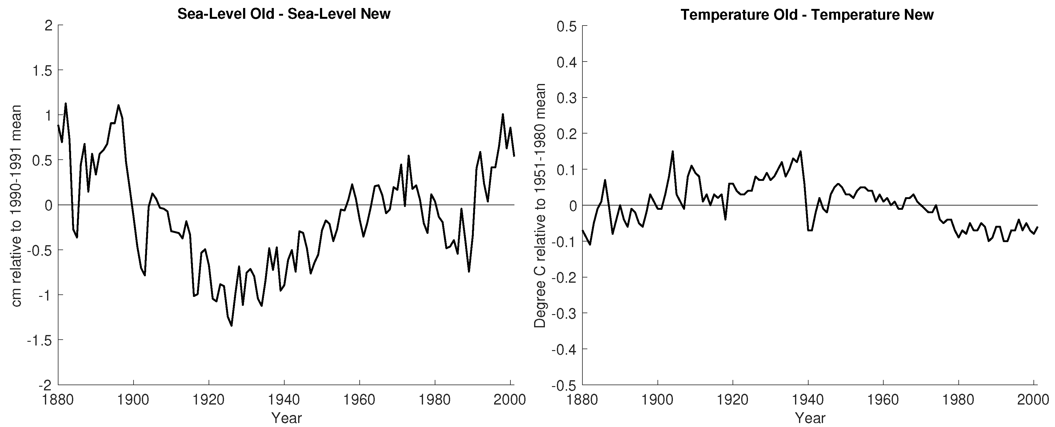
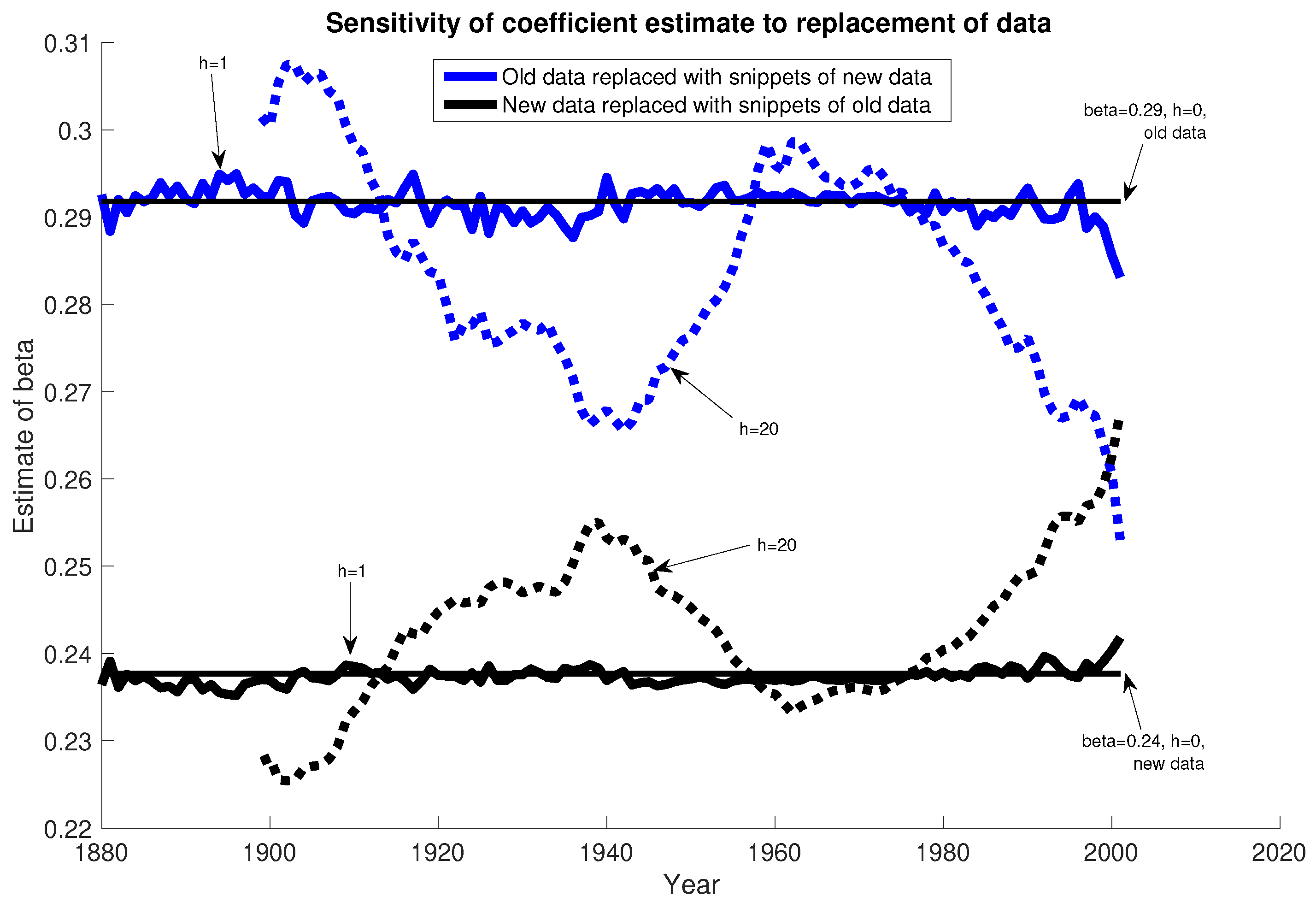
In Figure 7 the differences and are plotted for 1880 to 2001. We note that there are intervals where the different vintages give systematically different values. In order to investigate the influence of these differences on the estimates, we conduct the following exercise: Using the old data, we consecutively replace observation pair for to N with the corresponding pair from the new data set. We similarly replace observation pairs with the corresponding pairs from the new data set. Then we estimate the models proposed in Grassi et al. (2013); Schmith et al. (2012); Vermeer and Rahmstorf (2009) on each of these mixed data sets of temperature and sea level time series and record the estimated regression slope or , respectively. For h = 1 or 20, we obtain a time series of regression coefficients indexed from h to N that show the estimated slope if a moving window of h observations is replaced with new data. Then we do the same with the new data and consecutively replace with h-snippets of old data. Figure 8 shows the results for coefficients and Figure 9 shows b in the model proposed in Vermeer and Rahmstorf (2009). Figure 10 shows the results for the coefficient in the model proposed in Grassi et al. (2013) and Figure 11 shows in the Schmith et al. (2012) model. The results for the Rahmstorf (2007) model are very similar to those for the coefficient and are not reported here.
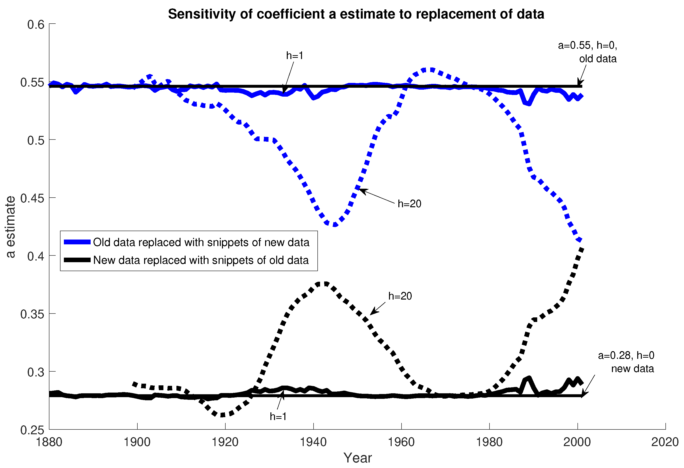
Figure 8 shows that for the Vermeer and Rahmstorf (2009) model, the periods 1920–1960 and the last 15 years of the record, 1985–2001, are the periods that influence the estimated coefficient most, but just replacing one observation has little effect, so we focus on replacing observations. We see that in the period 1920 to 1960 where the diffference is negative, interchanging 20 observations can change the parameter estimates drastically. For both these periods, the estimate of moves towards an agreement in the altered old and new data series. The curves of the estimated coefficients b overlap, so for this coefficient, replacing new data into the old series, and vice versa, can lead to an agreement of the estimated b-coefficient.
While the difference in the coefficient estimate between the old and the new vintage is smaller in the Grassi et al. (2013) model than in the Vermeer and Rahmstorf (2009) model, the Grassi et al. (2013) model is more sensitive to replacement of the snippets of size , as seen in Figure 10. The model estimates the coefficient on yearly data and does not pre-average the data into bins. Here the curves resulting from inserting new data snippets into the old time series and from inserting old data snippets into the new time series intersect both in the 1910–1950 period and during the last 15 years. in the early 1900s, there is a period of a few years where inserting old data into the new data series actually moves the estimated coefficient far into the opposite direction of the estimate on the new data and into the negative region.
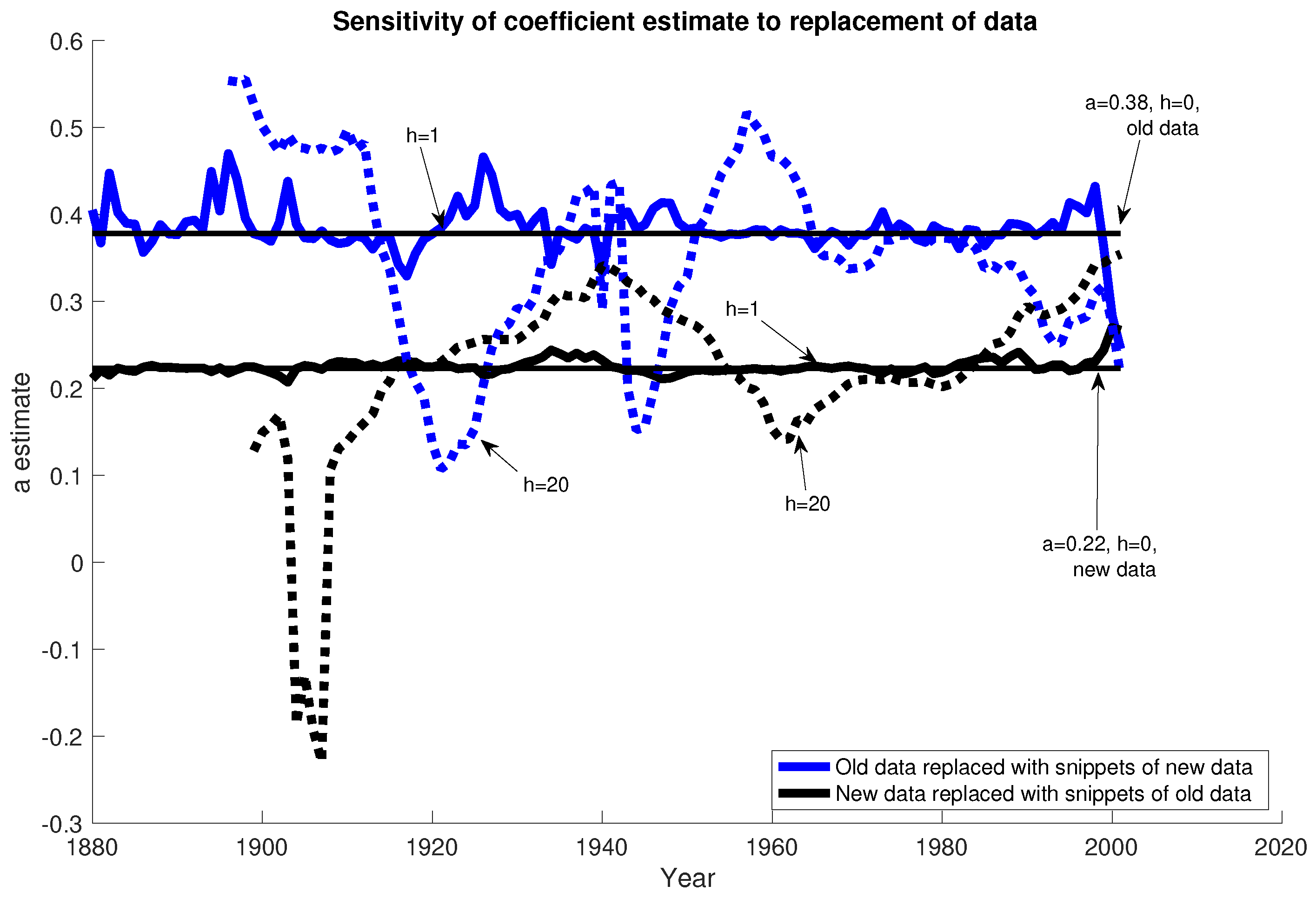
Figure 11 shows that the model proposed in Schmith et al. (2012) also reacts to the revisions in the data around the 1910s to 1950s and again in the 1990s. Towards the end of the sample period the families of -curves overlap. The range of the estimated coefficient, between approximately 0.23 and 0.31, is narrower than in the case of the Vermeer and Rahmstorf (2009) and closer to the discrepancy in the Grassi et al. (2013) model.
5. Conclusions
We have studied the influence of revisions of global mean temperature and global mean sea level data on the estimated statistical relation between the two series. We find that four alternative models proposed in the literature are sensitive to these data revisions, with substantial changes in the coefficient estimate that relates sea level to temperature (differences of up to 50%). These changes in the parameter estimates translate to substantial changes in long-term sea level projections obtained from temperature scenarios (differences of up to 40 cm). This shows that in order to replicate earlier results that informed the scientific discussion and motivated policy recommendations, it is crucial to work with the data vintages that were available at the time.
Author Contributions
Conceptualization and methodology, software, formal analysis, writing and editing, E.H., S.J. and T.S.; visualization, E.H. All authors have read and agreed to the published version of the manuscript.
Funding
Eric Hillebrand acknowledges financial support from the Independent Research Fund Denmark under the project Econometric Modeling of Climate Change.
Acknowledgments
We would like to thank the editor Neil Ericsson and three anonymous referees for insightful comments that helped improve the paper. An earlier version of this paper was circulated as CREATES Research Paper 2015-23 as well as University of Copenhagen, Department of Economics Discussion Paper 15-09.
Conflicts of Interest
The authors declare no conflict of interest.
References
- Bolin, David, Peter Guttorp, Alex Januzzi, Daniel Jones, Marie Novak, Harry Podschwit, Lee Richardson, Aila Särkkä, Colin Sowder, and Aaron Zimmerman. 2015. Statistical prediction of global sea level from global temperature. Statistica Sinica 25: 351–67. [Google Scholar]
- Bruns, Stephan B., Zsuzsanna Csereklyei, and David I. Stern. 2020. A multicointegration model of global climate change. Journal of Econometrics 214: 175–97. [Google Scholar] [CrossRef]
- Calafat, Francisco, Don Chambers, and Michael Tsimplis. 2014. On the ability of global sea level reconstructions to determine trends and variability. Journal of Geophysical Research: Oceans 119: 1572–92. [Google Scholar] [CrossRef] [Green Version]
- Chao, Benjamin, Yun-Hao Wu, and Y. S. Li. 2008. Impact of artificial reservoir water impoundment on global sea level. Science 320: 212–14. [Google Scholar] [CrossRef] [Green Version]
- Church, John A., and Neil J. White. 2006. A 20th century acceleration in global sea-level rise. Geophysical Research Letters 33: L01602. [Google Scholar] [CrossRef]
- Church, John A., and Neil J. White. 2011. Sea-level rise from the late 19th to the early 21st century. Surveys in Geophysics 32: 585–602. [Google Scholar] [CrossRef] [Green Version]
- Church, John A., Neil J. White, Richard Coleman, Kurt Lambeck, and Jerry X. Mitrovica. 2004. Estimates of the regional distribution of sea-level rise over the 1950–2000 period. Journal of Climate 17: 2609–25. [Google Scholar] [CrossRef]
- Church, John A., Peter U. Clark, Anny Cazenave, Jonathan M. Gregory, Svetlana Jevrejeva, Anders Levermann, Mark A. Merrifield, Glenn A. Milne, R. Steven Nerem, Patrrick D. Nunn, and et al. 2013. Sea level change. In Climate Change 2013: The Physical Science Basis. Contribution of Working Group I to the Fifth Assessment Report of the Intergovernmental Panel on Climate Change. Edited by Thomas Stocker, Dahe Qin, Gian-Kaspar Plattner, Melinda M. B. Tignor, Simon Allen, Judith Boschung, Alexander Nauels, Yu Xia, Vincent Bex and Pauline M. Midgley. Cambridge and New York: Cambridge University Press. [Google Scholar]
- Desmet, Klaus, Robert E. Kopp, Scott A. Kulp, Dávid Krisztián Nagy, Michael Oppenheimer, Esteban Rossi-Hansberg, and Benjamin H. Strauss. 2020. Evaluating the economic cost of coastal flooding. American Economic Journal: Macroeconomics. forthcoming. [Google Scholar]
- Duffy, James, and David Hendry. 2017. The impact of integrated measurement errors on modeling long-run macroeconomic time series. Econometric Reviews 36: 568–87. [Google Scholar] [CrossRef] [Green Version]
- Durbin, James, and Siem Jan Koopman. 2012. Time Series Analysis by State Space Methods, 2nd ed. Oxford: Oxford University Press. [Google Scholar]
- Grassi, Stefano, Eric Hillebrand, and Daniel Ventosa-Santaulària. 2013. The statistical relation of sea-level and temperature revisited. Dynamics of Atmospheres and Oceans 64: 1–9. [Google Scholar] [CrossRef] [Green Version]
- Gregory, Jonathan M., Neil J. White, John A. Church, Mark F. P. Bierkens, Jason E. Box, Michiel R. Van den Broeke, J. Graham Cogley, Xavier Fettweis, Edward Hanna, Phillipe Huybrechts, and et al. 2013. Twentieth-century global-mean sea level rise: Is the whole greater than the sum of the parts? Journal of Climate 26: 4476–99. [Google Scholar] [CrossRef] [Green Version]
- Grinsted, Aslak, John Moore, and Svetlana Jevrejeva. 2010. Reconstructing sea level from paleo and projected temperatures 200 to 2100 AD. Climate Dynamics 34: 461–72. [Google Scholar] [CrossRef]
- Hansen, James E., D. Johnson, Andrew Lacis, Sergej Lebedeff, P. Lee, David H. Rind, and Gary L. Russell. 1981. Climate impact of increasing atmospheric carbon dioxide. Science 213: 957–66. [Google Scholar] [CrossRef] [PubMed] [Green Version]
- Hansen, James E., and Sergej Lebedeff. 1987. Global trends of measured surface air temperature. Journal of Geophysical Research 92: 13343–72. [Google Scholar] [CrossRef] [Green Version]
- Hansen, James E., Reto A. Ruedy, J. Glascoe, and Makiko Sato. 1999. GISS analysis of surface temperature change. Journal of Geophysical Research 104: 30997–1022. [Google Scholar] [CrossRef]
- Hansen, James E., Reto A. Ruedy, Makiko Sato, M. Imhoff, W. Lawrence, David Easterling, T. Peterson, and Thomas Karl. 2001. A closer look at United States and global surface temperature change. Journal of Geophysical Research 106: 23947. [Google Scholar] [CrossRef] [Green Version]
- Hansen, James E., Reto A. Ruedy, Makiko Sato, and Kwok-Wai Ken Lo. 2010. Global surface temperature change. Reviews of Geophysics 48: RG4004. [Google Scholar] [CrossRef] [Green Version]
- Hay, Carling C., Eric Morrow, Robert E. Kopp, and Jerry X. Mitrovica. 2015. Probabilistic reanalysis of twentieth-century sea-level rise. Nature 517: 481. [Google Scholar] [CrossRef]
- Hendry, David F. 1995. Dynamic Econometrics. Oxford: Oxford University Press. [Google Scholar]
- Holgate, Simon J., Andrew Matthews, Philip L. Woodworth, Lesley J. Rickards, Mark E. Tamisiea, Elizabeth Bradshaw, Peter R. Foden, Kathleen M. Gordon, Svetlana Jevrejeva, and Jeff Pugh. 2013. New data systems and products at the permanent service for mean sea level. Journal of Coastal Research 29: 493–504. [Google Scholar]
- IPCC. 2001. Climate change 2001: The scientific basis. In Contribution of Working Group I to the Third Assessment Report of the Intergovernmental Panel on Climate Change. Edited by John T. Houghton, Yihui Ding, David J. Griggs, Maria Noguer, Paul van der Linden, Dai Xiaosu, K. Maskell and Cathrine A. Johnson. Cambridge and New York: Cambridge University Press. [Google Scholar]
- IPCC. 2019. IPCC special report. In IPCC Special Report on the Ocean and Cryosphere in a Changing Climate. Edited by Hans-Otto Pörtner, Debra C. Roberts, Valèrie Masson-Delmotte, Panmao Zhai, Melinda M. B. Tignor, Elvira Poloczanska, Katja Mintenbeck, Andrès Alegria, Maike Nicolai, Andrew Okem and et al. Cambridge and New York: Cambridge University Press. [Google Scholar]
- NASA Goddard Institute for Space Studies. 2020. GISS Surface Temperature Analysis (GISTEMP) v4. Data Set Accessed 2009-07 and 2018-10. Available online: https://data.giss.nasa.gov/gistemp/ (accessed on 23 October 2020).
- Jackson, Luke P., Aslak Grinsted, and Svetlana Jevrejeva. 2018. 21st century sea-level rise in line with the Paris Accord. Earth’s Future 6: 213–29. [Google Scholar] [CrossRef] [Green Version]
- Johansen, Søren. 1996. Likelihood-Based Inference in Cointegrated Vector Autoregressive Models, 2nd ed. Oxford: Oxford University Press. [Google Scholar]
- Kopp, Robert E., Andrew C. Kemp, Klaus Bittermann, Benjamin P. Horton, Jeffrey P. Donnelly, W. Roland Gehrels, Carling C. Hay, Jerry X. Mitrovica, Eric D. Morrow, and Stefan Rahmstorf. 2016. Temperature-driven global sea-level variability in the common era. Proceedings of the National Academy of Sciences of the United States of America 113: E1434–41. [Google Scholar] [CrossRef] [PubMed] [Green Version]
- Masui, Toshihiko, Kenichi Matsumoto, Yasuaki Hijioka, Tsuguki Kinoshita, Toru Nozawa, Sawako Ishiwatari, Etsushi Kato, Priyadarshi R. Shukla, Yoshiki Yamagata, and Mikiko Kainuma. 2011. An emission pathway for stabilization at 6 wm2 radiative forcing. Climatic Change 109: 59–76. [Google Scholar] [CrossRef]
- Meinshausen, Malte, Steven J. Smith, Katherine Calvin, John S. Daniel, Mikiko L. T. Kainuma, Jean-Francois Lamarque, Kazuhiko Matsumoto, Stephen A. Montzka, Sarah C. B. Raper, Keywan Riahi, and et al. 2011. The RCP greenhouse gas concentrations and their extensions from 1765 to 2300. Climatic Change 109: 213–41. [Google Scholar] [CrossRef] [Green Version]
- Moore, John C., Aslak Grinsted, and Svetlana Jevrejeva. 2005. New tools for analyzing time series relationships and trends. Eos, Transactions American Geophysical Union 86: 226–32. [Google Scholar] [CrossRef]
- Morice, Colin P., John J. Kennedy, Nick A. Rayner, and Phil D. Jones. 2012. Quantifying uncertainties in global and regional temperature change using an ensemble of observational estimates: The HadCRUT4 data set. Journal of Geophysical Research 117: D08101. [Google Scholar] [CrossRef]
- Rahmstorf, Stefan. 2007. A semi-empirical approach to projecting future sea-level rise. Science 315: 368–70. [Google Scholar] [CrossRef] [Green Version]
- Rahmstorf, Stefan, Martin Vermeer, and Mahé Perrette. 2012. Testing the robustness of semi-empirical sea level projections. Climate Dynamics 39: 861–75. [Google Scholar] [CrossRef]
- Ray, Richard D., and Bruce C. Douglas. 2011. Experiments in reconstructing twentieth-century sea levels. Progress in Oceanography 91: 496–515. [Google Scholar] [CrossRef] [Green Version]
- Schmith, Torben, Søren Johansen, and Peter Thejll. 2007. Comment on “A semi-empirical approach to projecting future sea-level rise”. Science 317: 1866. [Google Scholar] [CrossRef] [Green Version]
- Schmith, Torben, Søren Johansen, and Peter Thejll. 2012. Statistical analysis of global surface temperature and sea level using cointegration methods. Journal of Climate 25: 7822–33. [Google Scholar] [CrossRef]
- Thomson, Allison M., Katherine V. Calvin, Steven J. Smith, G. Page Kyle, April Volke, Pralit Patel, Sabrina Delgado-Arias, Ben Bond-Lamberty, Marshall A. Wise, and Leon E. Clarke. 2011. RCP4.5: A pathway for stabilization of radiative forcing by 2100. Climatic Change 109: 77–94. [Google Scholar] [CrossRef] [Green Version]
- Vermeer, Martin, and Stefan Rahmstorf. 2009. Global sea level linked to global temperature. Proceedings of the National Academy of Sciences of the United States of America 106: 21527–32. [Google Scholar] [CrossRef] [Green Version]
- Vose, Russell S., Derek Arndt, Viva F. Banzon, David R. Easterling, Byron Gleason, Boyin Huang, Ed Kearns, Jay H. Lawrimore, Matthew J. Menne, Thomas C. Peterson, and et al. 2012. NOAA’s merged land–ocean surface temperature analysis. Bulletin of the American Meteorological Society 93: 1677–85. [Google Scholar] [CrossRef]
- Wada, Yoshihide, Min-Hui Lo, Pat J.-F. Yeh, John T. Reager, James S. Famiglietti, Ren-Jie Wu, and Yu-Heng Tseng. 2016. Fate of water pumped from underground and contributions to sea-level rise. Nature Climate Change 6: 777–80. [Google Scholar] [CrossRef] [Green Version]
- Zanna, Laura, Samar Khatiwala, Jonathan M. Gregory, Jonathan Ison, and Patrick Heimbach. 2019. Global reconstruction of historical ocean heat storage and transport. Proceedings of the National Academy of Sciences of the United States of America 116: 1126–31. [Google Scholar] [CrossRef] [Green Version]
| 1. | |
| 2. | |
| 3. | |
| 4. | https://www.cmar.csiro.au/sealevel/sl_data_cmar.html. CSIRO’s primary data archive for sea level is now http://research.csiro.au/slrwavescoast/sea-level/measurements-and-data/sea-level-data/. |
| 5. | Our data set is available at http://raw.githubusercontent.com/chisos9/data_public/master/data_sealevel_2018.csv. |
| 6. | The correction adds the deterministic function to the sea level time series, which is an estimate of the water impoundment in artificial reservoirs. |
Figure 1.
The left panel shows old (—) and new (⋯) data for temperature 1880 to 2001/2013. The right panel shows old (—) and new (⋯) data for sea level 1880 to 2001/2013.
Figure 1.
The left panel shows old (—) and new (⋯) data for temperature 1880 to 2001/2013. The right panel shows old (—) and new (⋯) data for sea level 1880 to 2001/2013.

Figure 2.
The left panel shows old (—) and new (⋯) first differences of temperature 1881 to 2001/2013. The correlation coefficient on the overlapping sample period is 0.951. The right panel shows old (—) and new (⋯) first differences of sea level 1881 to 2001/2013. The correlation coefficient on the overlapping sample period is 0.862.

Figure 3.
The left panel shows the old vintage of sea level without (—) and with (⋯) reservoir correction for 1880 to 2001. The right panel shows the new vintage of sea level without (—) and with (⋯) reservoir correction for 1880 to 2013.
Figure 3.
The left panel shows the old vintage of sea level without (—) and with (⋯) reservoir correction for 1880 to 2001. The right panel shows the new vintage of sea level without (—) and with (⋯) reservoir correction for 1880 to 2013.

Figure 4.
Long-term projections from the Rahmstorf (2007) model. The temperature scenarios used are from RCP4.5 and RCP6, and the model parameters used for the resulting sea level projections are those estimated on the different vintage configurations. Note that the projections for the configuration overlay with those of the configuration .

Figure 5.
Long-term projections from the Vermeer and Rahmstorf (2009) model. The temperature scenarios used are from RCP4.5 and RCP6, and the model parameters used for the resulting sea level projections are those estimated on the different vintage configurations.
Figure 5.
Long-term projections from the Vermeer and Rahmstorf (2009) model. The temperature scenarios used are from RCP4.5 and RCP6, and the model parameters used for the resulting sea level projections are those estimated on the different vintage configurations.

Figure 6.
Long-term projections from the Grassi et al. (2013) model. The model parameters used for simulating temperature paths and the resulting sea level projections are those estimated on the different vintage configurations (i.e., there is no given temperature scenario in this case, in contrast to the projections made for the Rahmstorf (2007); Vermeer and Rahmstorf (2009) models).

Figure 7.
The left panel shows the difference for sea level and the right panel the for temperature.
Figure 7.
The left panel shows the difference for sea level and the right panel the for temperature.

Figure 8.
The figure shows the coefficient in the model proposed in Vermeer and Rahmstorf (2009) when snippets of new data ( and ) are inserted into the old data (upper curves) and when snippets of old data are inserted into new data (lower curves). The unit of the coefficient is cm per year per degree Celsius.

Figure 9.
The figure shows the estimates of the coefficient b in the model proposed in Vermeer and Rahmstorf (2009) when snippets of new data ( and ) are inserted into the old data (upper curves) and when snippets of old data are inserted into new data (lower curves). The unit of the coefficient is cm per year per degree Celsius.

Figure 10.
The figure shows the estimates of the coefficient in the model proposed in Grassi et al. (2013) when snippets of new data ( and ) are inserted into the old data (upper curves) and when snippets of old data are inserted into new data (lower curves). The unit of the coefficients is cm per year per degree Celsius.

Figure 11.
The figure shows the estimates of the coefficient in the model proposed in Schmith et al. (2012) when snippets of new data ( and ) are inserted into the old data (upper curves) and when snippets of old data are inserted into new data (lower curves). The unit of the coefficients is cm per year per degree Celsius.


Table 1.
Estimation of in the Rahmstorf (2007) model for the five combinations of data, with standard errors in parentheses. The unit of the coefficients is cm per year per degree Celsius.
| Sea Level | |||
|---|---|---|---|
| Temperature | |||
Table 2.
Estimation of and b in the Vermeer and Rahmstorf (2009) model for the five combinations of data, with standard errors in parentheses. The unit of the coefficients is cm per year per degree Celsius.
Table 2.
Estimation of and b in the Vermeer and Rahmstorf (2009) model for the five combinations of data, with standard errors in parentheses. The unit of the coefficients is cm per year per degree Celsius.
| Sea Level | |||
|---|---|---|---|
| Temperature | |||
Table 3.
Estimation of the coefficient of influence of temperature on sea level in the model proposed in Grassi et al. (2013). The estimates of the variances of and from the model are omitted for brevity and available upon request. The confidence intervals in parentheses are found by simulation. The unit of the coefficients is cm per year per degree Celsius.
| Sea Level | |||
|---|---|---|---|
| Temperature | |||
Table 4.
Estimation of the cointegrating relation in the model proposed in Schmith et al. (2012), using all combinations of the old and new vintages for temperature and sea level. Standard errors are stated in parentheses. The unit of the coefficients in the table is cm per year per degree Celsius. The unit of as estimated from the cointegrating relation is cm per degree Celsius. In order to arrive at a unit that is comparable to the ones measured in the other models, we have divided by the number of years in the samples.
| Sea Level | |||
|---|---|---|---|
| Temperature | |||
Table 5.
Estimated adjustment coefficients and in the model proposed in Schmith et al. (2012), using all combinations of the old and new vintages for temperature and sea level. In parentheses we report t-ratios. The unit of the coefficients in the table is degree Celsius per year per cm.
Table 5.
Estimated adjustment coefficients and in the model proposed in Schmith et al. (2012), using all combinations of the old and new vintages for temperature and sea level. In parentheses we report t-ratios. The unit of the coefficients in the table is degree Celsius per year per cm.
| Sea Level | |||
| Temperature | |||
| Sea Level | |||
| Temperature | |||
Publisher’s Note: MDPI stays neutral with regard to jurisdictional claims in published maps and institutional affiliations. |
© 2020 by the authors. Licensee MDPI, Basel, Switzerland. This article is an open access article distributed under the terms and conditions of the Creative Commons Attribution (CC BY) license (http://creativecommons.org/licenses/by/4.0/).
Share and Cite
MDPI and ACS Style
Hillebrand, E.; Johansen, S.; Schmith, T. Data Revisions and the Statistical Relation of Global Mean Sea Level and Surface Temperature. Econometrics 2020, 8, 41. https://0-doi-org.brum.beds.ac.uk/10.3390/econometrics8040041
AMA Style
Hillebrand E, Johansen S, Schmith T. Data Revisions and the Statistical Relation of Global Mean Sea Level and Surface Temperature. Econometrics. 2020; 8(4):41. https://0-doi-org.brum.beds.ac.uk/10.3390/econometrics8040041
Chicago/Turabian StyleHillebrand, Eric, Søren Johansen, and Torben Schmith. 2020. "Data Revisions and the Statistical Relation of Global Mean Sea Level and Surface Temperature" Econometrics 8, no. 4: 41. https://0-doi-org.brum.beds.ac.uk/10.3390/econometrics8040041
Note that from the first issue of 2016, this journal uses article numbers instead of page numbers. See further details here.