Are Soybean Yields Getting a Free Ride from Climate Change? Evidence from Argentine Time Series Data

Abstract

We analyze the influence of climate change on soybean yields in a multivariate time-series framework for a major soybean producer and exporter—Argentina. Long-run relationships are found in partial systems involving climatic, technological, and economic factors. Automatic model selection simplifies dynamic specification for a model of soybean yields and permits encompassing tests of different economic hypotheses. Soybean yields adjust to disequilibria that reflect technological improvements to seed and crops practices. Climatic effects include (a) a positive effect from increased CO${}_2$ concentrations, which may capture accelerated photosynthesis, and (b) a negative effect from high local temperatures, which could increase with continued global warming.

1. Introduction

The effects of climate change on agriculture have been widely studied due to its strong dependence on climatic variables and the international concern regarding future global food production as outlined in the Stern review (Stern 2007). However, as Nordhaus (2013) suggests (based on the IPCC 4th Assessment Report), it is especially in the agricultural sector where the adaptation and mitigation processes have been taking place. Such processes are mainly driven by technological developments or management changes such as crop displacement, replacing those most affected by global warming with “modest warming” areas.

One important mitigating factor for agriculture comes from the so-called carbon fertilization effect. CO${}_2$ concentrations could have an important beneficial effect on crop yields due to their fertilizer properties as they increase the rate of photosynthesis in plants. According to Nordhaus (2013), multiple field studies found that doubling CO${}_2$ atmospheric concentrations would increase rice, wheat and soybean yields by 10–15 percent. For the case of Argentina, the third largest soybean producer and exporter worldwide, Magrin et al. (2005) found, using agronomic models, a 38% change in yields corresponding to climate change between 1930–60 and 1970–2000.

In this paper, we econometrically study the long-run determinants of soybean yields in Argentina in order to understand and measure the effect of global climate change, including in particular the mitigating effects of CO${}_2$ concentrations. We address CO${}_2$ fertilization by considering the global CO${}_2$ concentration1 given its long-lasting and rather uniformly distributed effects.

Furthermore, we took into account other potential determinants of crop yields suggested in the literature, e.g., variables reflecting technological developments and economic factors such as output and input prices. To achieve this goal, we first followed a partial system approach that has several advantages. It allowed us to take into account many potential determinants of soybean yield, to deal with collinearities when variables show trending behavior2 and also to evaluate their exogeneity when there could be feedbacks among the variables included in the models. Thus, we separately estimated long-run relationships due to climate, technological and economic factors. Then, we used an automatic selection algorithm, Autometrics,3 to evaluate the encompassing of the deviations from the long-run equilibrium obtained from the different partial systems.

Our findings provide evidence that soybean yields in the long run are mainly dominated by technology innovations variables, such as the evolution of no-till adoption and the incorporation of new seeds. However, we found that crop yields are affected by climate variables in the short run. Carbon fertilization has a positive and significant short-run effect, while local high temperatures during the plant growing season negatively affect yields.

This paper is organized as follows. Section 2 discusses different approaches to modeling crop yields that have been analyzed by a wide body of literature. Section 3 describes our data. Section 4 explains the econometric methodology. Section 5 presents and discusses our main results. The last section includes our final remarks.

2. Different Approaches to Modeling Crop Yields

Awareness of global warming has sparked renewed interest in studying the effects of climatic variables on the agricultural sector over the last decade. The assessment of climate change effects on crop yields and production has been a multidisciplinary topic. Economists, agronomists, meteorologists and other scientists have been intensively studying the subject. Each discipline has brought a distinctive approach to modeling agriculture.

In contrast to econometric studies, many of the agronomic analyses focus on estimating the effect of climate on crop yields using models based on controlled experiments that require greater knowledge of the plant physiology, climate conditions and soil properties. However, those studies only incorporate physical aspects of potential yield and typically do not consider technological and global factors.

Crop simulation models are also widely used in agronomy and meteorology to predict the future behavior of crop production and yields due to global and local climate changes. Several other agronomic studies have modeled the effects of climate change on a wide variety of crops and areas throughout the world, but at a micro (states or counties) level. Empirical research shows mixed evidence of the negative effect of climate changes on crop yields because there would be several factors that have partially reduced the harmful consequences of climate change. Adaptation, trade, the declining share over time of agriculture in the economy and, relevant to our study, the mitigating carbon fertilization affect (see Nordhaus 2013). Lobell and Burke (2010) summarized the sources of divergence among different estimated models to obtain a more robust picture. They concluded that statistical models, compared with process-based models, play an important role in anticipating the future impacts of climate change.

For a county-level panel, Chen et al. (2013) estimated the effects of climate change on corn and soybean yields in China. The authors found non-linearities and asymmetric relationships between yields and weather variables as suggested in the literature (Schlenker and Roberts 2009). They found that extreme high temperatures are always harmful to crop growth.

Lobell et al. (2011) studied how the change in climate trends influenced the yield of four major crops between 1980 and 2008. The authors found that corn and wheat yields showed adverse effects for the largest producers. The net impact on rice and soybean production was insignificant, with gains in some countries that balanced the losses of others. Most of the impacts were due to changes in temperature trends and not precipitation.

These results are consistent with many recent studies in which changes in temperature are more important than changes in rainfall, at least at the national and regional levels (Reilly and Schimmelpfennig 2000; Schlenker and Lobell 2010). Crop yield losses on the hottest days drive much of the effect of temperature (Schlenker and Roberts 2009). Furthermore, crops are more sensitive to extremely high temperatures, in particular during the plant growth stage (Auffhammer et al. 2012; Welch et al. 2010). Burke and Emerick (2016) found that US corn and soybeans are significantly and negatively affected by long-term changes in extremely high temperatures. Changes in short-term temperature extremes can be critical, especially if they coincide with the growth stage for many crops (Wheeler et al. 2000).

As stated by Auffhammer and Schlenker (2014), one of the greatest challenges in empirical analyses is the identification of adaptation responses to changes in climatic conditions. Many of the previous studies have focused on assessing the effect of climate variables on crop yields without controlling for other potential determinants. Empirical studies should not ignore or underestimate the effects of adaptation measures as a means to compensate for the adverse effects of climate change. Several adaptation measures, such as shifting planting dates or developing new crop varieties, have also been suggested and implemented to reduce vulnerability to the potential negative impacts of climate change (Cohn et al. 2016; Lobell et al. 2008).

Another body of literature analyzes the responsiveness of crop yields to price variations, that is, the estimation of the (positive) own-price and the (negative) input price elasticities. Expected crop prices may influence crop management practices, which are often difficult to measure. Changes in input and output prices affect incentives for the substitution of acres among crops or in agricultural land expansion. The sensitivity of crop yields to their own prices is an old empirical question (see Choi and Helmberger 1993; Houck and Gallagher 1976). More recently, Lobell et al. (2009) and Miao et al. (2015) discussed and empirically considered the price responsiveness of crop yields. Using a large panel dataset for the 1977–2007 period and controlling for the endogeneity of crop yields,4 Miao et al. (2015) found that, in the US, price increase has a statistically significant positive impact on corn, but not on soybean yields.

In this line, our econometric approach tries to encompass different groups of drivers that affect crop yields apart from climate change, as shown in Figure 1. We consider that soybean yields can be simultaneously influenced by climatic, technological and economic factors.

3. Data Description

Our dataset consists of annual series from 1971 to 2015 ($T=45$). The initial sample period resulted from two factors: (1) data availability, and (2) the emergence of soybeans as a relevant crop to Argentina by the early 70s.

Table 1. Data description.

Symbol	Description	Units	Source
y	Soybean yield	kg/ha	FAO
$cropland$	Arable land + land in permanent crops	ha	USDA
$irrigation$	Area equipped for irrigation	ha	USDA
$labour$	Agricultural labor, 1000 persons economically active in agriculture	units	USDA
$machinery$	Number of 40 CV tractor-equivalents in use	units	USDA
$fertilizer$	Fertilizer consumption, first principal component of N, P${}_2$O${}_5$ and K${}_2$O	tonnes	IFA
$C{O}_2$	Mean atmospheric carbon dioxide at Mauna Loa Observatory, Hawaii	ppm	NOAA
$temp$	Global annual temperature anomalies	${}^{\circ }$C	CDIAC
$max28$	Number of days during growing season with maximum temperature above 28 ${}^{\circ }$C	days	SMN
$max29$	Number of days during growing season with maximum temperature above 29 ${}^{\circ }$C	days	SMN
$max30$	Number of days during growing season with maximum temperature above 30 ${}^{\circ }$C	days	SMN
$max31$	Number of days during growing season with maximum temperature above 31 ${}^{\circ }$C	days	SMN
$CV$	Precipitation coefficient of variation	%	SMN
$PCI$	Precipitation concentration index	%	SMN
$RGI$	Rainfall Gini Index	index	SMN
$AD$	Precipitation absolute deviations with respect to the historical mean	mm	SMN
$AD1SE$	AD ± one standard error	mm	SMN
$AD2SE$	AD ± two standard errors	mm	SMN
$Ni\tilde{n}a$	Niña events	dummy	BOM
$Ni\tilde{n}o$	Niño events	dummy	BOM
$notill$	Proportion of no tilled cropland acres	ratio	AAPRESID
$seeds$	Number of soybean seeds registered in Argentina, Brazil and United States	units	INASE, SRNC & USDA
$p^{fertilizer}$	Weighted average of natural phosphate rock, phosphate, potassium, and nitrogenous prices. Based on current US dollars	2010 = 100	World Bank
$p^{land}$	Agricultural land value	US$/ha	Márgenes Agropecuarios
$p^{soybean}$	Soybean prices. Based on current US dollars	2010 = 100	World Bank

reports the variables’ descriptions and sources.

Demand for oilseeds, and particularly soybeans, has rapidly increased over the last decades. It is one of the world’s most valuable crops, not only because of its use as oil seed but also as a high-protein meal for animal and human consumption, as well as a source for biofuel production. In Argentina, the third largest producer of soybeans worldwide, its production increased by 2.5% annually from 1971 to 2015. Average soybean yield (measured as kilogram per hectare, kg/ha) increased from 1624 kg/ha in 1971 to 3175 kg/ha in 2015. During the sample period, climate changes and technological advances shifted the main production area to the north, to warmer latitudes.

3.1. Climate Variables

Several global and local climate variables are considered in the analysis. One of the best predictors for soybean yield is a measure of extreme heat during growth periods considering a temperature threshold above 30 ${}^{\circ }$C in the US Schlenker and Roberts (2009). Using daily data on maximum temperature from 54 meteorological stations from the soybean production area, we created different variables that measure the number of days in a year during the crop growth stage (from December to April) in which the temperature exceeded a threshold of 28, 29, 30 or 31 ${}^{\circ }$C. We evaluated which of these different thresholds has a significant impact on Argentine soybean yields as detailed in the next section. The maximum temperature from each meteorological station was weighted by its share in the total soybean planted area. Such weights were annually updated to account for the displacement of crop areas over time.5

Another weather influence on crop yields is precipitation. Unfavorable weather conditions during the plant growing season may threaten soybean yields. We used the daily precipitation data from the same meteorological stations from the soybean production area, as described above, to evaluate different measures of excess or lack of precipitation. We restricted our analysis to the stages in which the plant reaches the full pod stage and the seed development begins. We include: the coefficient of variation ($CV$), the precipitation concentration index ($PCI$), the rainfall Gini index ($RGI$), the absolute deviations with respect to the historical mean ($AD$), the AD plus and minus one standard error ($AD1SE$), and the AD plus and minus two standard errors ($AD2SE$).

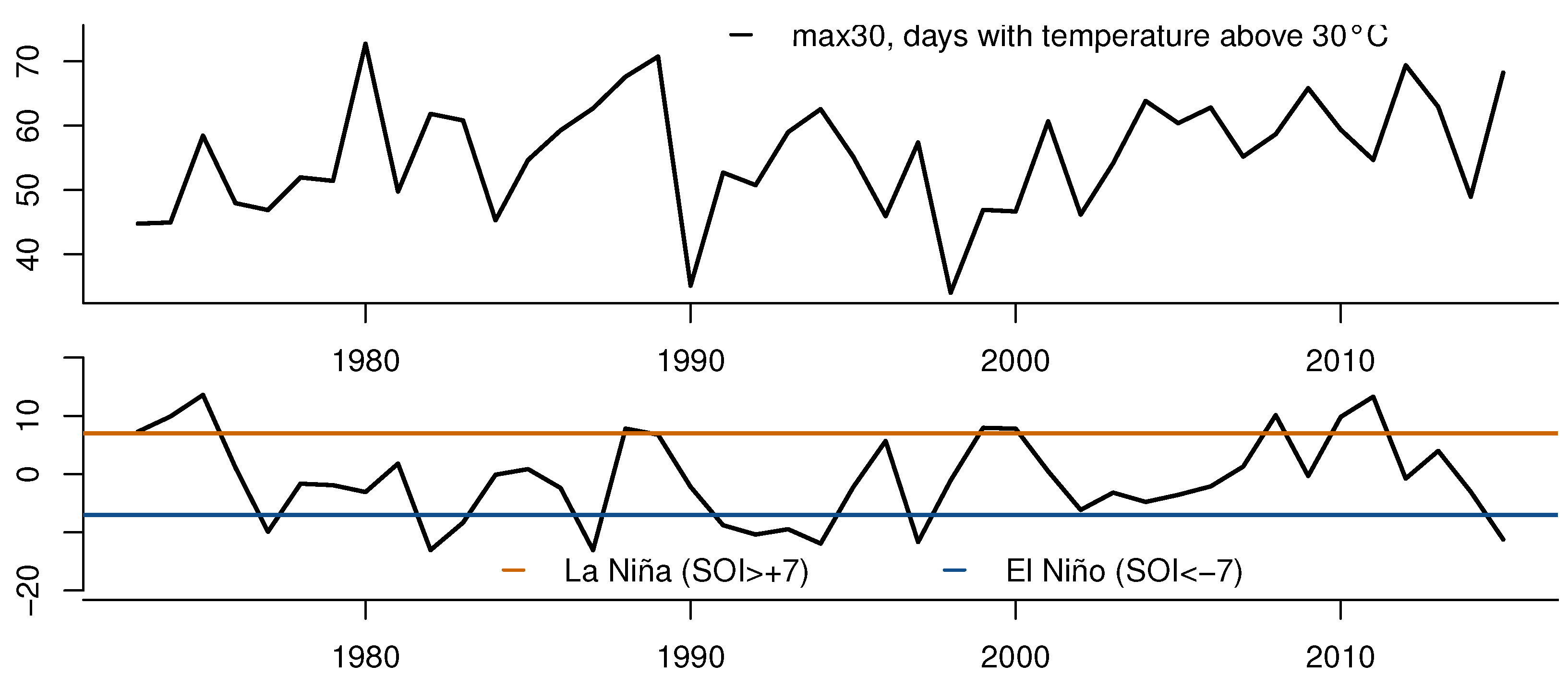
Additionally, El Niño and La Niña phenomena in the Pacific Ocean were identified through the Southern Oscillation Index (SOI), which is calculated using the pressure differences between Tahiti and Darwin. Sustained negatives values of SOI below −7 indicate El Niño episodes, while sustained positives values of SOI above +7 indicate La Niña episodes (see Figure 2). El Niño and La Niña phenomena are respectively associated with floods and droughts in southeastern South America.

We also considered a global warming measure: the global temperature anomalies computed from land and ocean data as the temperature differences (in ${}^{\circ }$C) relative to the 1951–1980 base period means reported by the GISTEMP team of the Carbon Dioxide Information Analysis Center (CDIAC). During our sample period, the global temperature anomalies showed a steady increase from a minimum of −0.81 ${}^{\circ }$C in 1974 to a maximum of 0.86 ${}^{\circ }$C by 2015. Global temperatures can have other long-run negative effects on crops, such as the development of plagues and pests, which are difficult to measure.

Carbon dioxide (CO${}_2$) levels in the atmosphere produced by increasing anthropogenic emissions may have positive effects on plant growth, as plants use carbon dioxide in photosynthesis. Carbon fertilization has a greater effect on plants with C4 and C3 photosynthesis systems (such as corn and soybeans, respectively), which can concentrate carbon dioxide in reaction sites. However, this effect may not take place as nutrient levels, soil moisture, water availability and other conditions must also be met. The simulation study of Gray et al. (2016) found that the intensification of drought eliminates the potential benefits of elevated dioxide for soybeans.

Figure 3 shows the evolution of soybean yields, global temperature anomalies and the global CO${}_2$ concentration on the surface during the analyzed period.

3.2. Other Potential Determinants of Soybean Yields

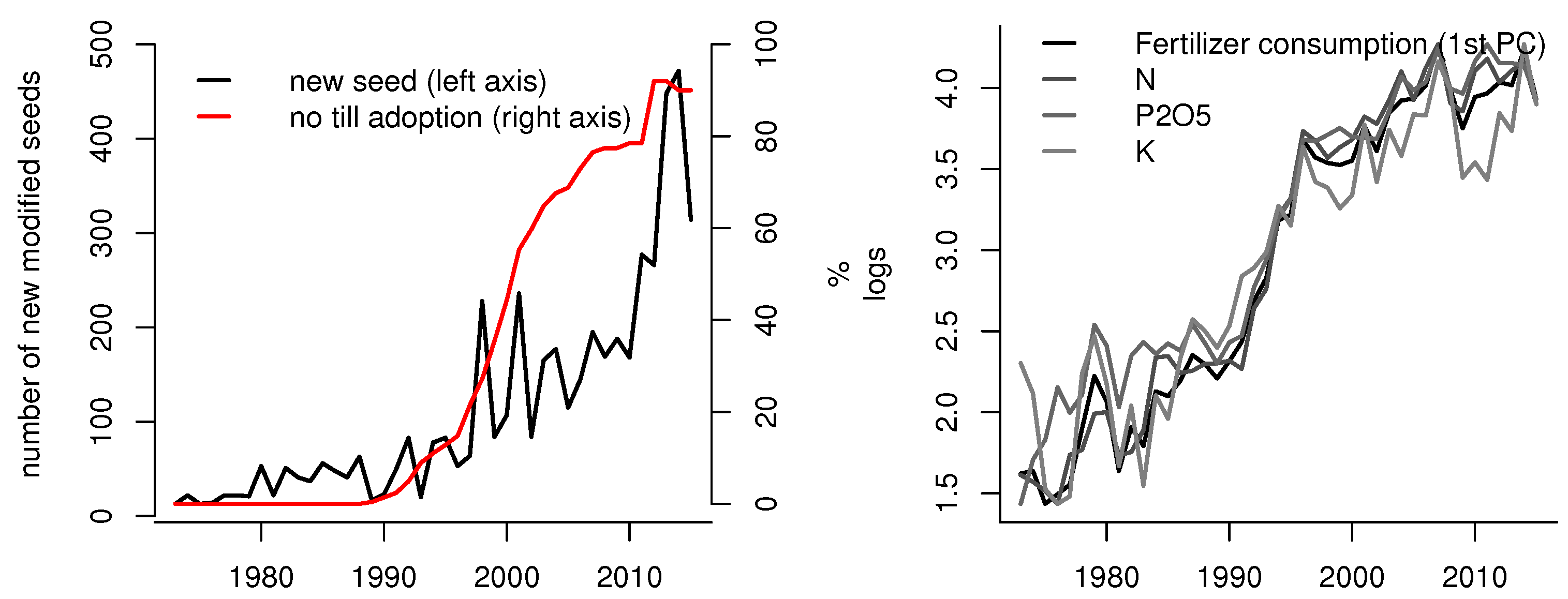
To control for other determinants, we also considered the consumption of different fertilizers. Soybean plants usually require large amounts of phosphorus ($P_2{O}_5$) and potassium ($K_{2}O$) and, to a lesser extent, nitrogen (N). In order to have an aggregate measure of fertilizer use and to control for the fertilizers’ high collinearities (Figure 4), we have conducted a principal component analysis among the consumption of these three fertilizers and obtained the first principal component accounting for 96.94% of data variability that was then incorporated into our models.

To assess the effect of changes in management practices, we included the evolution of no till practices, which has rapidly gained ground in Argentina as an effective solution to soil erosion problem.

The use of new modified seeds was also considered in our analysis through the number of soybean varieties registered in the United States, Brazil and Argentina (the world’s three largest soybean producers). This variable intends to capture the knowledge transfer across the three leading countries in soybean production from the adoption of genetically modified (GM) crops. Commercially grown GM soybeans are concentrated in those three countries. Figure 4 shows the marked trend for many of the technological variables. Other input factors, such as agricultural and irrigated land, machinery use and agricultural labor, were included, but were not statistically significant.

Finally, our dataset also includes prices to address the elasticity of soybean yield response with respect to output and input prices (such as fertilizers prices or agricultural land prices).

4. Econometric Methodology

In order to study the effects of many potential crop-yield drivers, we adopted a cointegration approach working with partial systems that allowed us to deal with dimensionality, collinearities and endogeneity issues.

This methodology was first implemented by Juselius (1992), Brouwerde Brouwer and Ericsson (1998) and Hendry (2001) to model inflation considering the complicated relationships in different markets. From the estimation of separated systems, different equilibrium relationships were obtained and their deviations were used to explain inflation dynamics. In our case, this approach can be fruitful to estimate crop yields using the three kinds of models shown in Figure 1: climate, technological and economic systems. By estimating three different systems, we used a multivariate cointegration approach to model the long-run behavior of soybean yields.

A great advantage of this approach is “the invariance of the cointegration property to extensions of the information set. This means that if cointegration is found between a set of variables, this cointegration result will remain valid if more variables are added to the analysis” (Juselius 2006, p. 349). This specific to general strategy helps identify and interpret long-run structure with plausible equilibrium correction coefficients in the case of multivariate cointegration, particularly when the sample is relatively short.

The cointegrated systems also allow us to distinguish between influences that move equilibria (pushing forces) and influences that correct deviations from equilibrium (pulling forces), which give rise to long-run relationships. After determining the cointegration rank, the significance of adjustment coefficients provides information on which variables adjust and thereby weak exogeneity can be tested by zero restrictions in the respective coefficients. In this way we can address the endogeneity issue.

To sum up, the idea of estimating partial systems consists in using cointegration analysis of smaller blocks of variables as a means to restructure and simplify the empirical problem. Then, those systems can be combined into a full model that includes all the deviations from the estimated long-run equilibria to find out which disequilibria in different sectors affect the variable of interest (e.g., soybean yields). We tested if one or more deviations are significant by means of the concept of encompassing (Hendry and Mizon 1993).

We started by estimating the three different partial systems from Figure 1 (named climate, technological, and input–output prices). We estimated VAR models with two lags. Given that the variables may grow at different rates, we initially included a trend in the cointegration space and, if not significant, its effect is restricted to zero. All variables are expressed in logs, with the exception of global temperature anomalies ($temp$), the number of days with maximum temperatures above 28, 29, 30 and 31 ${}^{\circ }$C ($max28$, $max29$, $max30$ and $max31$, respectively) and the ratio of no tillage adoption ($notill$).

It should be noted that some of the series used in these systems can be represented as stationary around a deterministic linear trend (

Table 2. Unit root tests.

Variable	Trend	k	ADF	b	PP	b	KPSS
$lny$	yes	0	−7.00 ***	2	−6.99 ***	2	0.08
$temp$	yes	0	−5.91 ***	5	−5.85 ***	4	0.05
ln CO${}_2$	yes	0	−1.11	3	−1.03	5	0.20 **
$max30$	no	0	−6.17 ***	3	−6.23 ***	3	0.27
$AD2SE$	no	0	−5.84 ***	1	−5.84 ***	2	0.22
$Ni\tilde{n}a$	no	0	−5.19 ***	2	−5.22 ***	3	0.13
$lnseeds$	yes	0	−4.57 ***	0	−4.57 ***	3	0.11
$notill$	yes	1	−1.76	3	−1.68	5	0.20 **
$ln{p}^{fertilizer}$	yes	0	−3.05	5	−3.02	4	0.13 *
$ln{p}^{soybean}$	yes	0	−2.83	2	−2.86	4	0.14 *
$ECter{m}^{climate}$	no	0	−5.68 ***	2	−5.68 ***	3	0.15
$ECter{m}^{technology}$	no	0	−5.16 ***	3	−5.29 ***	4	0.17
$ECter{m}^{prices}$	no	0	−5.27 ***	1	−5.28 ***	5	0.22
$\Delta lny$	no	1	−7.69 ***	8	−16.11 ***	20	0.21
$\Delta temp$	no	6	−5.30 ***	20	−21.08 ***	44	0.50
$\Delta ln$ CO${}_2$	no	0	−5.45 ***	1	−5.43 ***	2	0.69 **
$\Delta max30$	no	1	−8.63 ***	9	−18.30 ***	7	0.14
$\Delta AD2SE$	no	1	−8.68 ***	21	−23.70 ***	20	0.22
$\Delta Ni\tilde{n}a$	no	1	−7.20 ***	7	−13.85 ***	12	0.16
$\Delta lnseeds$	no	1	−7.74 ***	0	−9.28 ***	0	0.09
$\Delta notill$	no	0	−3.86 ***	2	−3.79 ***	4	0.42 *
$\Delta ln{p}^{fertilizer}$	no	1	−6.28 ***	11	−6.13 ***	10	0.16
$\Delta ln{p}^{soybean}$	no	1	−6.12 ***	13	−5.81 ***	10	0.15
$\Delta ECter{m}^{climate}$	no	2	−6.99 ***	40	−25.72 ***	24	0.27
$\Delta ECter{m}^{technology}$	no	0	−11.43 ***	8	−15.88 ***	6	0.13
$\Delta ECter{m}^{prices}$	no	1	−8.05 ***	44	−20.28 ***	31	0.34

Note: k = lag length selected by SIC, b = bandwidth using Bartlett kernel. *, ** and *** indicate significance at the 10%, 5% and 1% levels, respectively. ADF = Augmented Dickey Fuller, PP = Phillips–Perron, KPSS = Kwiatkowski–Phillips–Schmidt–Shin. A constant and a trend were included for level variables that exhibited a trend behavior, otherwise only a constant was considered.

). To tackle this issue, many studies have removed deterministic trends before studying the effects of climate factors on yields (see for example Thomasz et al. 2016, in the Argentine case). However, given that our aim is to understand which variables could be behind this observed trending behavior, we studied their long-run relationships assuming them as first-order integrated, and studying cointegration. As Juselius (2006, p. 18) assessed, “the order of integration of a variable is not in general a property of an economic variable but a convenient statistical approximation to distinguish between the short-run, medium-run and long-run variation in the data”.

In the climatic system, we estimated the interdependencies among non-stationary variables: soybean yields, CO${}_2$ concentrations in the atmosphere and global temperature anomalies. We have also unrestrictedly included La Niña and El Niño measures as well as stationary weather variables associated with excessive precipitations and floods, and different maximum temperature thresholds (28, 29, 30 and 31 ${}^{\circ }$C). To select the stationary variables and, in particular, the relevant maximum temperature threshold, we used Autometrics, as explained below, keeping the non-stationary variables and their lags fixed in the soybean yield equation of the VAR. Only La Niña and $max30$ were significant.

In the technological system, we considered the potential long-run interaction between soybean yields and two major technological advances in Argentina’s agricultural sector: the used of GM seeds and the adoption of no-till practices. This partial system also includes a step dummy starting in 1996 (as the main changes in managerial practices took place in the mid 1990s), which is restricted to enter the cointegration space, and two unrestricted impulse dummies for 2001 and 2002 (associated with the Argentine economic crisis). Those dummies were selected using Step and Impulse Indicator Saturation (SIS and IIS, respectively) at a 0.001 significance level.6 As stated by Castle et al. (2015), unmodeled location shifts can have pernicious effects on the constancy of models and may lead to misspecification problems. In our context, the latter may affect which variables may have a long-run relationship with soybean yields.7

Finally, the input–output prices system intends to model how soybean prices and several input prices affect the long-run behavior of soybean yields. Soybean and fertilizer prices showed a significant long-run effect on yields. This system also includes three unrestricted impulse dummies for 1971, 1972 and 1973, which may be related to the initial stages of soybeans in Argentina and the international oil crises that affected most of the commodity prices.

Once the long-run relationships were identified, their results were combined into an equilibrium correction (EC) model that nests all deviations from the long-run equilibria along with many potential short-run determinants from our information set. A key assumption of this approach is that the variable of our interest is affected by the relative magnitude of these deviations.

Formally, for the log differences of soybean yields ($\Delta y_t$), the estimated equation is:

$$\Delta y_t=\gamma +\sum _{j=1}^3{\alpha }_j\left[y_{t-1}-{\beta }_j^{\prime }{x}_{jt-1}\right]+\sum _{k=1}^1{\rho }_k\Delta y_{t-k}+\sum _{k=0}^1{\lambda }^{\prime }{w}_{t-k}+{\epsilon }_t$$

(1)

where $j=1,\cdots ,3$ indicates each of the partial systems. In (1), vector $x_j$ denotes the variables that enter each j partial system; ${\alpha }_j$ and ${\beta }_j$ denote the adjustment coefficients and long-run coefficient for the j partial system, respectively. We considered up to a $k=1$ lag for the w variables entering the short-run.8

To deal with such a wide range of information and help us select the dominant congruent model and not only the best fit, we used Autometrics.9 Moreover, this algorithm can be used for an encompassing evaluation, as discussed by Doornik (2008), selecting the relevant model(s) from a general unrestricted model, which includes all the variables of the different models obtained.

5. Results

In this section, we present the results obtained using the information set described in Section 3 and following the econometric approach explained in Section 4.

5.1. Long-Run Effects

Considering the different kinds of potential determinants of crop yields, we estimated the three partial systems of Argentine soybean yields in line with the description of Figure 1.

Table 3. Cointegration analysis for the climatic subsystem.

Cointegration Rank r	$\mathit{r}=0$	$\mathit{r}\le 1$	$\mathit{r}\le 2$	$\mathit{r}\le 3$
Log-likelihood	327.18	338.75	348.44	352.53
Eigenvalue	–	0.40	0.35	0.17
Null hypothesis	$r=0$	$r\le 1$	$r\le 2$
Trace statistics (bootstrap)	50.71	27.57	8.19
	[0.063]	[0.103]	[0.261]
Trace statistics (Bartlett)	46.89	24.79	7.44
	[0.017]	[0.066]	[0.310]
Variable	$lny$	$lntemp$	ln CO${}_2$	$trend$
Restricted cointegrating vector	1	1.60	−9.21	0
	(–)	(0.61)	(2.23)	(–)
Adjustment coefficients	−0.32	−0.24	−0.002
	(0.10)	(0.09)	(0.001)
Likelihood ratio statistic ${\chi }^2\left(1\right)$	2.40 [0.12]

Notes. The VAR(2) model includes Nina_t−1 and max30_t unrestrictedly. Estimated standard errors are in parentheses; p-values are in square brackets.

,

Table 4. Cointegration analysis for the technological subsystem.

Cointegration Rank r	$\mathit{r}=0$	$\mathit{r}\le 1$	$\mathit{r}\le 2$	$\mathit{r}\le 3$
Log-likelihood	−118.36	−95.83	−86.14	−78.11
Eigenvalue	–	0.72	0.36	0.24
Null hypothesis	$r=0$	$r\le 1$	$r\le 2$
Trace statistics (bootstrap)	90.75	32.33	12.55
	[0.000]	[0.040]	[0.070]
Trace statistics (Bartlett)	80.69	26.11	10.24
	[0.000]	[0.056]	[0.134]
Variable	$lny$	$lnseeds$	$no-till$	$S1996$	$trend$
Restricted cointegrating vector	1	−0.11	−0.008	−0.55	0
	(–)	(0.02)	(0.001)	(0.09)	(–)
Adjustment coefficients	−0.39	–	8.76
	(0.16)	–	(1.48)
Likelihood ratio statistic ${\chi }^2\left(2\right)$	2.09 [0.35]

Notes. The VAR(2) model unrestrictedly includes two impulse dummies: I2001 and I2002. Estimated standard errors are in parentheses; p-values are in square brackets.

and

Table 5. Cointegration analysis for the prices subsystem.

Cointegration Rank r	$\mathit{r}=0$	$\mathit{r}\le 1$	$\mathit{r}\le 2$	$\mathit{r}\le 3$
Log-likelihood	61.10	81.47	91.86	94.68
Eigenvalue	–	0.60	0.37	0.12
Null hypothesis	$r=0$	$r\le 1$	$r\le 2$
Trace statistics (bootstrap)	67.16	26.42	5.64
	[0.013]	[0.080]	[0.504]
Trace statistics (Bartlett)	62.44	24.90	5.41
	[0.000]	[0.064]	[0.548]
Variable	$lny$	$ln{p}^{fertilizer}$	$ln{p}^{soybeans}$	$trend$
Cointegrating vector	1	1.29	−1.84	−0.02
	(–)	(0.19)	(0.30)	(0.004)
Adjustment coefficients	−0.22	−0.37	0.27
	(0.09)	(0.17)	(0.09)

Notes. The VAR(2) model unrestrictedly includes three impulse dummies: I1971, I1972 and I1973. Estimated standard errors are in parentheses; p-values are in square brackets.

report statistics p-values for the cointegration analysis considering a bootstrap estimation of each cointegrated partial system, and also applying a Bartlett small-sample correction for the rank tests. Additionally, the (not rejected by our data) constrained parameter estimates are reported.

We can observe that only one cointegration relation is determined in each partial system using a 5% level of significance. Equations (2)–(4) show the resulting long-run equations for the cases in which the yield adjusts. Equation (2) shows the long-run relationship corresponding to the climatic model. Equation (3) belongs to the technology model describing the long-run relationship of yields with the effects of no-till adoption and the introduction of new seed varieties. Finally, Equation (4) corresponds to the price model.

$$\begin{array}{cc}\hfill (\mathrm{climatic}\mathrm{model})& lny=-1.60temp+9.21lnC{O}_2\hfill \end{array}$$

(2)

$$\begin{array}{cc}\hfill (\mathrm{technological}\mathrm{model})& lny=0.008notill+0.11lnseeds+0.55S1996\hfill \end{array}$$

(3)

$$\begin{array}{cc}\hfill (\mathrm{prices}\mathrm{model})& lny=1.84ln{p}^{soybean}-1.29ln{p}^{fertilizer}+0.02t\hfill \end{array}$$

(4)

First, as much of the literature does, we focus only on climate variables. Global temperature anomalies and atmospheric CO${}_2$ concentrations were found to be cointegrated with soybean yields. An interesting feature is that, although global temperature had a negative effect, the results suggest a mitigating effect on yield associated with carbon fertilization. To analyze the magnitude of estimated coefficients, it is worth noting that in this sample period, if the temperature changes as its median value (0.06 ${}^{\circ }$C), soybean yields will decrease by almost 10% in the long run. As a possible mitigating effect, yields increased by about 4% as a consequence of the median percentage variations of CO${}_2$ concentrations (0.47%) during 1971–2015.

In this system, soybean yields adjusted to deviations from the long-run relationship as well as global temperature anomalies and CO${}_2$ concentrations. Although this last result may be unexpected at first sight, it may be due to the effect of deforestation. We can note that the upward trend of yields in Argentina is also shown by other main soybean producers like Brazil. Increasing yields could have given incentives to the expansion of agriculture through the use of new lands coming from deforestation. South America, during our sample period, has experienced a shift of the main production area to the north, to warmer latitudes, mainly by converting forest into crop land. Deforestation contributes to global warming since it reduces atmospheric CO${}_2$ concentrations, which could (at least partially) offset carbon dioxide anthropogenic emissions. Global temperature anomalies and CO${}_2$ concentrations may also adjust to deviations from our estimated climate long-run relationship. As Pretis (2021) warns, human activity (e.g., through deforestation) affects the local and global climate and climate change, in turn, influences human activity (e.g., crop yields). Empirically, this implies that if we want to estimate the effect of humanity on climate change and vice versa, it is essential to evaluate the exogeneity of the variables within the economic-climatic system.

Nonetheless, we have found other representations associated with factors different from climate change. A system including the main technological innovations for crop practices was studied. One long-run relationship was found in which soybean yields are explained by the no-till adoption measure and the introduction of new seeds, in both cases with positive effects.10 In this system, soybean yields and no-till adoption adjust to deviations from the long run.

Finally, in accordance with the price model, the commodity price and a main variable input price—fertilizers—have shown the expected signs.11 From the prices system, we found that all variables adjust to deviations from the long-run equilibrium.

The estimated Equations (2)–(4) suggest that to understand crop yield behavior in the long, run not only are climate variables important, but technological and economic factors should be considered too. Consistent estimates of the long-run effects can be obtained from these systems, given the cointegration approach.

5.2. Short-Run Effects

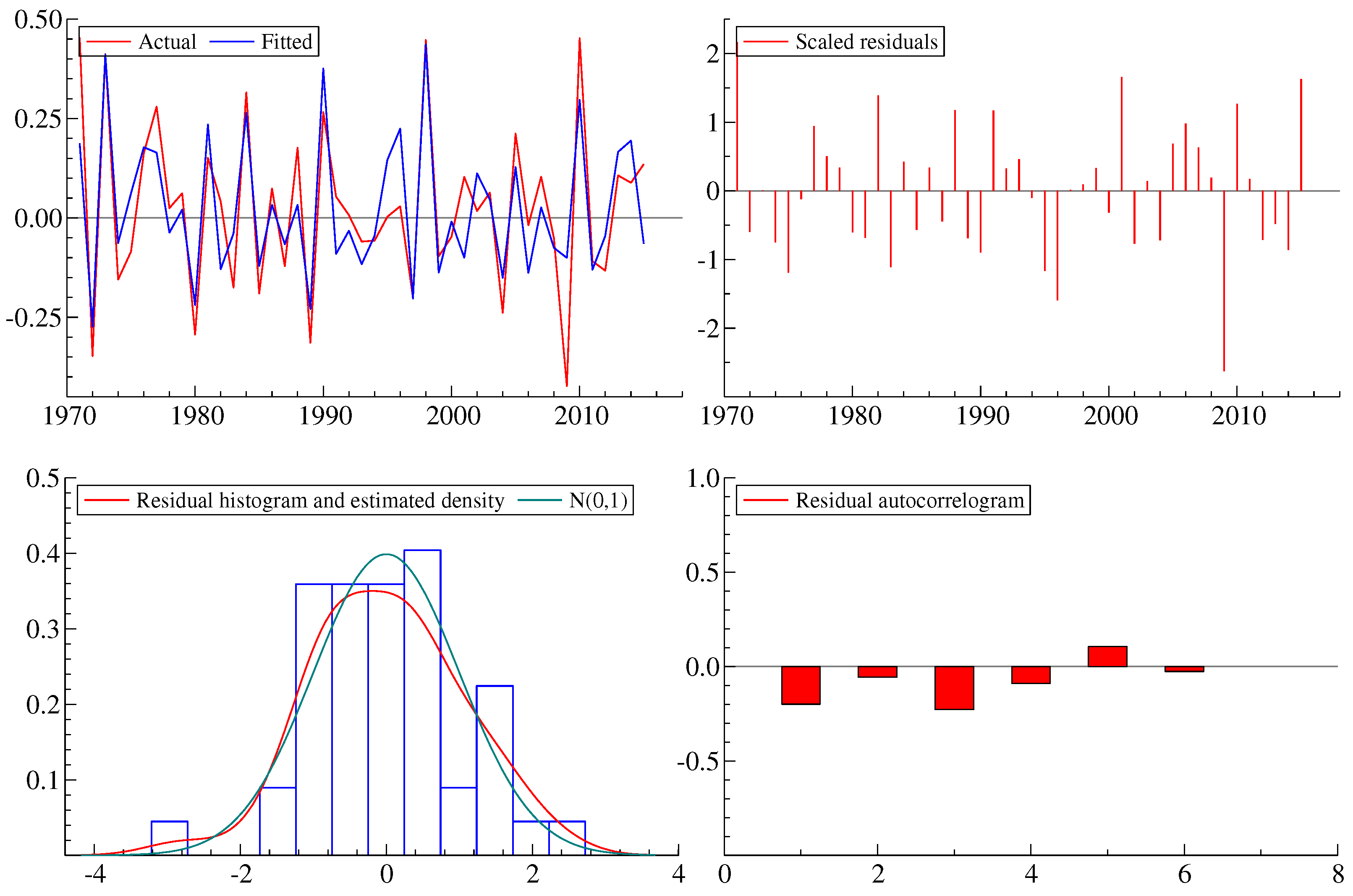
In consequence, we have several explanations, which may be alternative or complementary, to account for the long-run trending behavior of soybean yields. Encompassing by automatic selection can help discriminate long-run effects while selecting other, short-run, determinants. Results are presented in

Table 6. Selected equilibrium correction model, 1971–2015.

Dependent Variable ($\mathbf{\Delta }\mathit{ln}\left(\mathit{y}\right)$)	OLS	IV
	(1)	(2)	(3)
$constant$	2.80	2.85	4.32
	(0.75)	(0.78)	(5.59)
	[0.00]	[0.00]	[0.77]
$\Delta ln{\left(C{O}_2\right)}_t$	38.45	62.67	61.71
	(13.77)	(29.57)	(28.34)
	[0.00]	[0.04]	[0.04]
$max{30}_t$	−0.012	−0.013	−0.012
	(0.002)	(0.002)	(0.002)
	[0.00]	[0.00]	[0.00]
$\Delta ln{\left(y\right)}_{t-1}$	−0.29	−0.24	−0.27
	(0.11)	(0.13)	(0.14)
	[0.01]	[0.07]	[0.06]
EC term${}_{t-1}^{technology}$	−0.34	−0.36	−0.34
	(0.11)	(0.12)	(0.13)
	[0.00]	[0.00]	[0.01]
EC term${}_{t-1}^{climate}$			0.03
			(0.11)
			[0.29]
EC term${}_{t-1}^{prices}$			−0.07
			(0.07)
			[0.27]
$\widehat{\sigma }$	0.123	0.127	0.128
${\chi }^2$ test of excluded instruments		80.36	84.29
		[0.00]	[0.00]
Sargan test		2.34	1.73
		[0.51]	[0.19]
AR 1-2 F-test	1.35	0.76	0.40
	[0.27]	[0.47]	[0.67]
ARCH 1-1 F-test	0.00	0.04	0.20
	[0.95]	[0.84]	[0.66]
Normality ${\chi }^2\left(2\right)$ test	1.10	1.90	0.58
	[0.58]	[0.39]	[0.75]
Heteroskedasticity F-test	0.74	0.88	1.08
	[0.66]	[0.33]	[0.41]

Note: standard errors reported in parentheses, p-values in brackets.

and residual diagnostics in Figure 5.

Column (1) shows the Ordinary Least Squares (OLS) estimation of the model selected by Autometrics at the 1% target size.12 Column (2) shows the instrumental variable (IV) estimation, as the variation of CO${}_2$ concentrations has contemporaneous effects on yield variations. From the long-run results presented in Section 5.1, CO${}_2$ concentrations also adjusted to reach the equilibrium in the climatic model, and thus it is necessary to address the potential endogeneity issue. Therefore, for the EC representation, we re-estimated the model using instrumental variables. As instruments, we employed the log difference of the global fossil fuel consumption13 and its first lag, the log level of passenger cars and commercial vehicles14 and its first lag. According to the CDIAC, hundreds of billions of tons of carbon have been released into the atmosphere from the consumption of fossil fuels since 1751, leading to a positive correlation between these two variables. Finally, Column (3) incorporates the EC terms of the climate and prices model, which were not selected by Autometrics. As indicated in Table 6, the estimated models pass all diagnostic tests at traditional levels. The Sargan test validates the instrumental variables, as the null hypothesis that the error term is not correlated with the instruments is not rejected.

The main finding is that only the EC term derived from the technology model maintains its effect on soybean yield when nested with other long-run deviations. Therefore, the results obtained from this in-sample encompassing test performed by Autometrics suggest that the information content of the technology model in the long run is such that it dominates the others.

However, the effect of climate variables can also explain yield variation in the short run. Our estimates show that an increase in CO${}_2$ concentration growth produces higher soybean yields. For the median values of CO${}_2$ increases, the short-run effect on yield is about 18% (for the OLS estimation) and 29% (for the IV estimation), all else equal. However, it is difficult to assume that atmospheric CO${}_2$ concentrations could rise without an increase in global temperature and a higher intensity, frequency and duration of extreme weather events. The estimates show also the negative effects of cumulated days of high temperature. Ten additional days of maximum temperature above 30 ${}^{\circ }$C during the growing season produce a decrease of around 10%.

Although it is difficult to assess how the climate variables in this model will change in the future due to the local consequences of global warming, the free ride effect of Argentine soybean yields should be jointly evaluated with the potential effects derived from other climate variables.

6. Final Remarks

This paper has focused on understanding the effects of climate change on crop yields, and in particular if there is evidence of a beneficial effect of CO${}_2$ fertilization in the case of soybeans. We followed an econometric approach that enabled us to evaluate this hypothesis considering other climatic, technological and economic factors that have been examined in the literature to describe crop yields. It is a difficult task, mainly due to many different potential determinants, collinearities and endogeneity. A partial system approach allowed us to deal with these issues and study the long-run behavior of soybean yields for the world’s third largest producer and exporter of this commodity. Specifically, we estimated a system to measure the effect of global climate change along with the mitigating effects driven by atmospheric CO${}_2$ concentrations. Two other systems were also estimated to analyze: (i) the effects coming from new management practices and technology innovations, (ii) output and input prices. Once these different models for the long-run relationships were obtained, we used an automatic algorithm, Autometrics, to evaluate which of the deviations of the equilibria is relevant to explain changes in soybean yields, also including short-run effects. This analysis helped us verify if one representation can encompass others or whether none of them can do it.

Our main results indicate that soybean yields in the long run are mainly dominated by technology innovation variables, such as the evolution of no-till adoption and the incorporation of new seeds. As short-run determinants, we found positive effects from changes in atmospheric CO${}_2$ concentrations, which would suggest a climate change mitigation. Nonetheless, we also found negative climate effects from high temperatures during the plant growing season in line with the existing literature. Extreme events, which affect crop yields, are likely to be consequences of global warming as well and, thus, they should be jointly evaluated when analyzing climate change effects.

As part of the future agenda, further research should focus on studying if the technological long-run drivers of soybean yields have been a result of economic factors or part of an adaptation process to the same climate factors derived from global warming.

References

- Auffhammer, Maximilian, Veerabhadran Ramanathan, and Jeffrey R. Vincent. 2012. Climate change, the monsoon, and rice yield in India. Climatic Change 111: 411–24. [Google Scholar] [CrossRef]
- Auffhammer, Maximilian, and Wolfram Schlenker. 2014. Empirical studies on agricultural impacts and adaptation. Energy Economics 46: 555–61. [Google Scholar] [CrossRef] [Green Version]
- Brouwerde Brouwer, Gordon, and Neil R. Ericsson. 1998. Modeling inflation in Australia. Journal of Business & Economic Statistics 16: 433–49. [Google Scholar] [CrossRef]
- Burke, Marshall, and Kyle Emerick. 2016. Adaptation to climate change: Evidence from US agriculture. American Economic Journal: Economic Policy 8: 106–40. [Google Scholar] [CrossRef] [Green Version]
- Castle, Jennifer, Jurgen Doornik, David Hendry, and Felix Pretis. 2015. Detecting location shifts during model selection by step-indicator saturation. Econometrics 3: 240–64. [Google Scholar] [CrossRef] [Green Version]
- Chen, Shuai, Xiaoguang Chen, and Jintao Xu. 2013. Impacts of climate change on corn and soybean yields in China. Paper present at 2013 AAEA & CAES Joint Annual Meeting, Washington, DC, USA, August 4–6. [Google Scholar]
- Choi, Jung-Sup, and Peter G. Helmberger. 1993. How sensitive are crop yields to price changes and farm programs? Journal of Agricultural and Applied Economics 25: 237–44. [Google Scholar] [CrossRef] [Green Version]
- Cohn, Avery S., Leah K. VanWey, Stephanie A. Spera, and John F. Mustard. 2016. Cropping frequency and area response to climate variability can exceed yield response. Nature Climate Change 6: 601. [Google Scholar] [CrossRef]
- Doornik, Jurgen, and Katarina Juselius. 2017. Cointegration Analysis of Time Series Using CATS 3 for OxMetrics. London: Timerlake Consultants Ltd. [Google Scholar]
- Doornik, Jurgen A. 2008. Encompassing and automatic model selection. Oxford Bulletin of Economics and Statistics 70: 915–25. [Google Scholar] [CrossRef]
- Doornik, Jurgen A. 2009. Autometrics. In The Methodology and Practice of Econometrics. A Festschrift in Honour of David Hendry. Edited by Jennifer Castle and Neil Shephard. Oxford: Oxford University Press, pp. 88–121. [Google Scholar]
- Gray, Sharon B., Orla Dermody, Stephanie P. Klein, Anna M. Locke, Justin M. Mcgrath, Rachel E. Paul, David M. Rosenthal, Ursula M. Ruiz-Vera, Matthew H. Siebers, and Reid Strellner. 2016. Intensifying drought eliminates the expected benefits of elevated carbon dioxide for soybean. Nature Plants 2: 16132. [Google Scholar] [CrossRef]
- Hendry, David F. 2001. Modelling UK inflation, 1875–1991. Journal of Applied Econometrics 16: 255–75. [Google Scholar] [CrossRef]
- Hendry, David F., and Jurgen A. Doornik. 2014. Empirical Model Discovery and Theory Evaluation: Automatic Selection Methods in Econometrics. Cambridge: MIT Press. [Google Scholar]
- Hendry, David F., and Grayham E. Mizon. 1993. Evaluating Dynamic Econometric Models by Encompassing the VAR. Oxford: University of Oxford, pp. 272–300. [Google Scholar]
- Houck, James P., and Paul W. Gallagher. 1976. The price responsiveness of US corn yields. American Journal of Agricultural Economics 58: 731–34. [Google Scholar] [CrossRef]
- Juselius, Katarina. 1992. Domestic and foreign effects on prices in an open economy: The case of Denmark. Journal of Policy Modeling 14: 401–28. [Google Scholar] [CrossRef]
- Juselius, Katerina. 2006. The Cointegrated VAR Model. Methodology and Applications. Oxford: Oxford University Press. [Google Scholar]
- Lobell, David. 2010. Crop responses to climate: Time-series models. In Climate Change and Food Security. Edited by David Lobell. Dordrecht: Springer, pp. 85–98. [Google Scholar]
- Lobell, David B., and Marshall B. Burke. 2010. On the use of statistical models to predict crop yield responses to climate change. Agricultural and Forest Meteorology 150: 1443–52. [Google Scholar] [CrossRef]
- Lobell, David B., Marshall B. Burke, Claudia Tebaldi, Michael D. Mastrandrea, Walter P. Falcon, and Rosamond L. Naylor. 2008. Prioritizing climate change adaptation needs for food security in 2030. Science 319: 607–10. [Google Scholar] [CrossRef] [PubMed]
- Lobell, David B., Kenneth G. Cassman, and Christopher B. Field. 2009. Crop yield gaps: Their importance, magnitudes, and causes. Annual Review of Environment and Resources 34: 179–204. [Google Scholar] [CrossRef] [Green Version]
- Lobell, David B., Wolfram Schlenker, and Justin Costa-Roberts. 2011. Climate trends and global crop production since 1980. Science, 1204531. [Google Scholar] [CrossRef] [PubMed] [Green Version]
- Magrin, Graciela O., María I. Travasso, and Gabriel R. Rodríguez. 2005. Changes in climate and crop production during the 20th century in Argentina. Climatic Change 72: 229–49. [Google Scholar] [CrossRef]
- Miao, Ruiqing, Madhu Khanna, and Haixiao Huang. 2015. Responsiveness of crop yield and acreage to prices and climate. American Journal of Agricultural Economics 98: 191–211. [Google Scholar] [CrossRef] [Green Version]
- Nordhaus, William D. 2013. The Climate Casino: Risk, Uncertainty, and Economics for a Warming World. New Haven: Yale University Press. [Google Scholar]
- Pretis, Felix. 2021. Exogeneity in Climate Econometrics. Energy Economics 96: 105122. [Google Scholar] [CrossRef]
- Reilly, John, and David Schimmelpfennig. 2000. Irreversibility, uncertainty, and learning: Portraits of adaptation to long-term climate change. Climatic Change 45: 253–78. [Google Scholar] [CrossRef]
- Schlenker, Wolfram, and David B. Lobell. 2010. Robust negative impacts of climate change on African agriculture. Environmental Research Letters 5: 014010. [Google Scholar] [CrossRef]
- Schlenker, Wolfram, and Michael J Roberts. 2009. Nonlinear temperature effects indicate severe damages to US crop yields under climate change. Proceedings of the National Academy of Sciences 106: 15594–98. [Google Scholar] [CrossRef] [PubMed] [Green Version]
- Stern, Nicholas. 2007. The Economics of Climate Change. The Stern Review. Cambridge: Cambridge University Press. [Google Scholar]
- Suits, Daniel B. 1955. An econometric model of the watermelon market. American Journal of Agricultural Economics 37: 237–51. [Google Scholar] [CrossRef]
- Thomasz, Esteban Otto, María Teresa Casparri, Ana Silvia Vilker, Gonzalo Rondinone, and Miguel Fusco. 2016. Medición económica de eventos climáticos extremos en el sector agrícola: El caso de la soja en Argentina. Revista de Investigación en Modelos Financieros 2: 30–57. [Google Scholar]
- Welch, Jarrod R., Jeffrey R. Vincent, Maximilian Auffhammer, Piedad F. Moya, Achim Dobermann, and David Dawe. 2010. Rice yields in tropical/subtropical Asia exhibit large but opposing sensitivities to minimum and maximum temperatures. Proceedings of the National Academy of Sciences 107: 14562–67. [Google Scholar] [CrossRef] [Green Version]
- Wheeler, Timothy R., Peter Q. Craufurd, Richard H. Ellis, John R. Porter, and P. V. Vara Prasad. 2000. Temperature variability and the yield of annual crops. Agriculture, Ecosystems & Environment 82: 159–67. [Google Scholar] [CrossRef]
Figure 1.
Determinants of crop yields.
Figure 2.
Number of days with temperatures above 30 C during the growing season and El Niño and La Niña phenomena.
Figure 3.
Soybean yields in Argentina and global climate variables.
Figure 4.
Technological variables evolution.
Figure 5.
Fitted and actual values of from OLS estimation in Table 6, and the corresponding scaled residuals, residual histogram and estimated density, and residual correlogram.