Selecting a Model for Forecasting

Abstract

We investigate forecasting in models that condition on variables for which future values are unknown. We consider the role of the significance level because it guides the binary decisions whether to include or exclude variables. The analysis is extended by allowing for a structural break, either in the first forecast period or just before. Theoretical results are derived for a three-variable static model, but generalized to include dynamics and many more variables in the simulation experiment. The results show that the trade-off for selecting variables in forecasting models in a stationary world, namely that variables should be retained if their noncentralities exceed unity, still applies in settings with structural breaks. This provides support for model selection at looser than conventional settings, albeit with many additional features explaining the forecast performance, and with the caveat that retaining irrelevant variables that are subject to location shifts can worsen forecast performance.

1. Introduction

There are many approaches to formulating models when the sole objective is forecasting, from the very parsimonious through to large systems. However, there is little agreement on which performs best on a forecasting criterion: see Makridakis and Hibon (2000) and Fildes and Ord (2002) for evidence from forecast competitions. Clements and Hendry (2001) suggest that this lack of agreement is the result of intermittent distributional shifts that affect alternative formulations in different ways. We address this puzzle by analysing the selection of models in the pursuit of optimal mean square forecast error (MSFE) in settings with structural breaks.1

We focus on regression models that are linear in the parameters, and consider model selection that is controlled by the nominal significance level for statistical significance. Loose significance levels have been shown to be optimal to select regression models for stationary processes if evaluating on a one-step-ahead MSFE. Shibata (1980) showed that the Akaike information criterion (AIC, see Akaike 1973) is an asymptotically efficient selection method when the data generating process (DGP) is an infinite-order process; also see Ing and Wei (2003). Many other criteria have been proposed that aim to have optimal properties in certain settings but information criteria alone are not a sufficient principle for selecting models as they do not ensure congruence, so a misspecified model could be selected: see Bontemps and Mizon (2003). We explore general-to-specific (Gets) model selection in the simulation exercise to narrow down the class of forecasting models to undominated models. This yields well-specified encompassing models in sample, albeit nonstationarities may preclude those benefits continuing over the forecast horizon.

The theoretical analysis commences with a bivariate conditional model that is part of a three-variable system in which the selection decision is whether to retain or exclude one of the regressors. This is empirically relevant as demonstrated by UK inflation, where autoregressive (AR) forecasting models are augmented with the unemployment rate. The bivariate model is analysed first in a stationary setting. This is extended to a nonstationary settings where location shifts occur at or near the forecast origin. The static setting still requires forecasts of the conditioning variables, and alternative forecasting devices are considered, including the two extremes of the class of robust forecasting devices proposed by Castle et al. (2015), the sample mean and the random walk. The results confirm that regressors should be retained for forecasting if their noncentralities exceed unity, regardless of whether or not there is a structural break, or of the forecasting device used. These analytic results map to a selection significance level of 16% in the bivariate case, much looser than conventional significance levels used. The results closely match that of AIC, which can be interpreted as a likelihood ratio ${\chi }^2$ test for a pair of nested models with one degree of freedom and a penalty of two, and also gives a significance level of approximately 16%: see Pötscher (1991) and Leeb and Pötscher (2009).

A key source of forecast failure is an induced shift in the equilibrium mean of the variable being forecast, irrespective of whether those conditioning variables are included in the forecasting model; see the taxonomy in Hendry and Mizon (2012). Consequently, the simulation exercise evaluates a wide range of settings including larger models, break types and magnitudes at or near the forecast origin, and the method of forecasting. We consider a range of significance levels from the very tight (0.001), eliminating almost all potentially irrelevant variables, to the very loose (0.50), enabling retention of relevant variables even if they are only marginally significant. The results enable evaluation of the costs when either omitting relevant variables, or from incorrectly retaining irrelevant variables. Overall, the results support looser than conventional significance levels for selecting forecasting models, with a 10% target significance level often producing superior forecasts.

This paper is structured as follows. Section 2 outlines the aims of this paper, then Section 3 formulates the model framework that is analysed. Section 4 considers the choice of selection significance level for forecasting in a stationary DGP. Section 5 analyses selection in a nonstationary DGP where a location shift occurs out of sample in one of the regressors, and investigates the consequences of that variable’s inclusion or exclusion in the forecasting model. Section 6 considers the impacts on selection of in-sample shifts using different forecasting devices. The analytic results are summarized in Section 7. Section 8 and Section 9 present simulation design and evidence on the performance of the various approaches, examining the preferred significance level to minimize MSFE across experimental designs. Section 10 concludes this paper. Appendix A provides analytical calculations and Supplementary Tables are given in Appendix B.

2. Empirical Motivation

An empirical example of inflation forecasting motivates our interest in structural breaks and their roles in forecast accuracy and the selection of regressors. Two popular models within this large literature include single-equation forecasting models based on past inflation and so-called ‘Phillips curve forecasts’. The former usually consist of univariate models such as autoregressive integrated moving average (ARIMA) models. In the latter, the univariate model is augmented with an activity variable such as the unemployment rate or output gap; see Stock and Watson (2009).

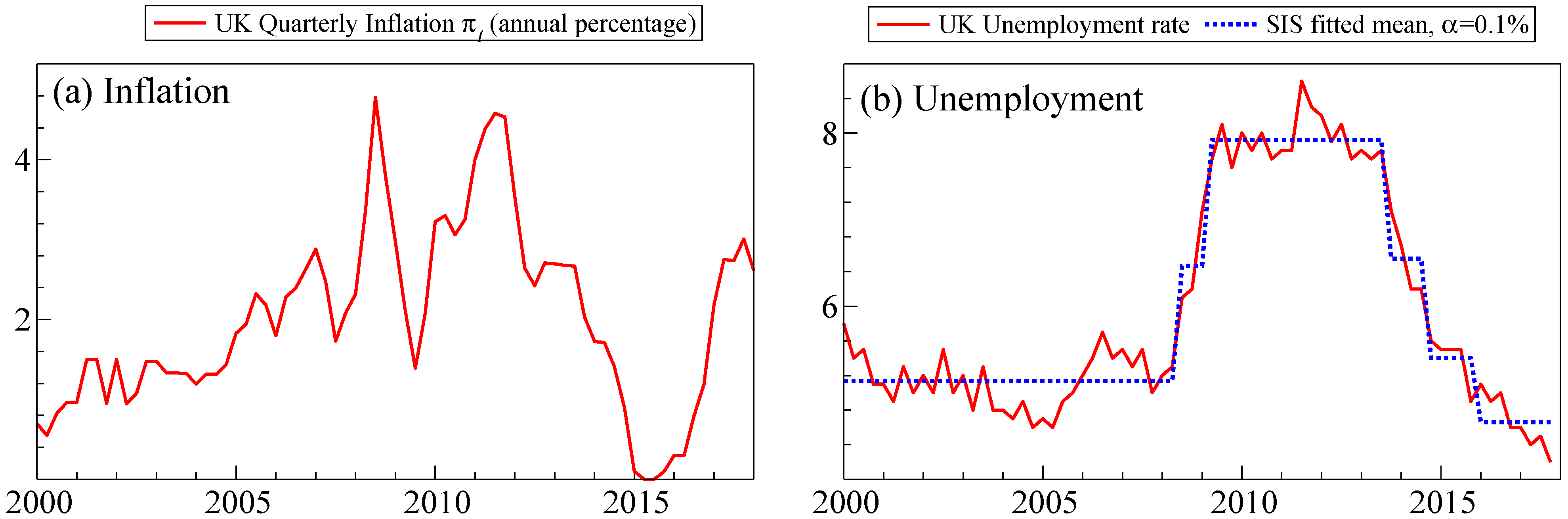
The framework considered below, although static, can be applied to these two models where the econometrician wishes to determine whether to augment a univariate forecasting model with the contemporaneous unemployment rate. This ‘exogenous’ variable is subject to breaks in the form of location shifts, which may occur at or near the forecast horizon. Figure 1 records2 the quarterly observations on the annual percentage inflation in UK consumer price index, ${\pi }_t$, and the UK unemployment rate as a percentage, $U_t$, along with a broken mean obtained by step indicator saturation (SIS, see Castle et al. 2015) at a nominal significance level $\alpha =0.1\%$.

The analytics derived below correspond to a Phillips curve formulation (model ${\mathrm{M}}_1$), a univariate AR model (${\mathrm{M}}_2$) and selection applied to the unemployment rate using a significance level of 0.16 (${\mathrm{M}}_3$). Using model-specific coefficients $\mu ,{\beta }_i,{\gamma }_i$ and error term ${\nu }_i$, the three models are:

$$\begin{array}{cc}\hfill {\mathrm{M}}_1:& \Delta {\pi }_t=\mu +{\sum }_{i=1}^4{\beta }_i\Delta {\pi }_{t-i}+{\sum }_{i=0}^4{\gamma }_i{U}_{t-i}+{\nu }_t,\hfill \\ \hfill {\mathrm{M}}_2:& \Delta {\pi }_t=\mu +{\sum }_{i=1}^4{\beta }_i\Delta {\pi }_{t-i}+{\nu }_t,\hfill \\ \hfill {\mathrm{M}}_3:& \Delta {\pi }_t=\mu +{\sum }_{i=1}^4{\beta }_i\Delta {\pi }_{t-i}+{\sum }_{i=0}^4{\gamma }_i^{*}{U}_{t-i}+{\nu }_t,\hfill \end{array}$$

where $\Delta {\pi }_t={\pi }_t-{\pi }_{t-1}$. Selection using Autometrics at $\alpha =0.16$ is denoted by ${}^{*}$, e.g., ${\gamma }_0^{*}=0$ implies that the contemporaneous unemployment rate is not selected. Dynamics are included to account for any autocorrelation. The forecasting models are estimated over the period 2000Q1–2013Q4, producing one-quarter-ahead inflation forecasts for the period 2014Q1–2017Q4 evaluated on MSFE. Selection at 16% results in $U_{t-1}$ being retained, with a p-value of 0.149, so would not be retained under a commonly used 5% significance level. Longer lags of the unemployment rate were not retained.

Table 1. Root mean square error of one-step forecast for $\Delta {\pi }_t$ over the period 2014Q1–2017Q4.

Conditioning on	M1	M2	M3
Known $U_t$	0.535	0.530	0.515
Mean forecast for $U_t$	0.519	0.530	0.542
Random walk forecast for $U_t$	0.549	0.530	0.515

reports the square root of the MSFEs (RMSFE) for one-step-ahead forecasts over the sample that was held back. Three cases are considered corresponding to the analytics below: (a) known $U_t$, (b) forecast ${\widehat{U}}_t$ using the in-sample mean, and (c) forecast ${\widehat{U}}_t$ using $U_{t-1}$. Method (a) is infeasible; method (c) is the random walk forecast. When $U_t$ is known, model ${\mathrm{M}}_3$ outperforms ${\mathrm{M}}_1$ and ${\mathrm{M}}_2$, although the differences are not statistically significant. As this is infeasible, the random walk forecast combined with selection matches the RMSFE of knowing $U_t$. This shows that selection can be beneficial. The next four sections formalize the framework to establish the optimal significance level for selection.

3. The Analytic Design

In this section, we specify the analytic design, consisting of a three-variable DGP and two different models for that DGP. In later sections, we introduce a third model that involves selection. Together, these mimic the models ${\mathrm{M}}_1$, ${\mathrm{M}}_2$, and ${\mathrm{M}}_3$ that were introduced above.

The DGP is a static vector autoregression (VAR) for variables $y,x_1,x_2$ with coefficients ${\beta }_i,{\mu }_i$ and error terms $ϵ,{\eta }_1,{\eta }_2$ structured as:

$$\left(\begin{array}{ccc}1& -{\beta }_1& -{\beta }_2\\ 0& 1& 0\\ 0& 0& 1\end{array}\right)\left(\begin{array}{c}{y}_t\\ x_{1,t}\\ x_{2,t}\end{array}\right)=\left(\begin{array}{c}{\beta }_0\\ {\mu }_1\\ {\mu }_2\end{array}\right)+\left(\begin{array}{c}{ϵ}_t\\ {\eta }_{1,t}\\ {\eta }_{2,t}\end{array}\right).$$

(1)

Using ${\mathbf{y}}_t^{\prime }=(y_t:x_{1,t}:x_{2,t})$ and ${\mathit{\mu }}^{\prime }=({\mu }_y:{\mu }_1:{\mu }_2)$, assuming normality, we can write (1) as:

$${\mathbf{y}}_t\sim {\mathrm{IN}}_3\left[\mathit{\mu },\mathsf{\Sigma }\right].$$

(2)

${\mathrm{IN}}_3$ denotes a three-dimensional independent normal distribution, here with mean $\mathit{\mu }$ and variance $\mathsf{\Sigma }$. Without loss of generality we set the variance of $x_1$ and $x_2$ to one, $\mathrm{V}\left[x_{i,t}\right]={\sigma }_{ii}^2=1$, and the correlation between $x_1$ and $x_2$ to $\rho$:

$$\mathsf{\Sigma }=\left(\begin{array}{ccc}{\sigma }_{ϵ}^2& 0& 0\\ 0& 1& \rho \\ 0& \rho & 1\end{array}\right).$$

(3)

Unless otherwise noted, Figure 2, Figure 3, Figure 4, Figure 5, Figure 6, Figure 7 and Figure 8 use the following parameter values in calculations: ${\beta }_0=5$, ${\beta }_1=1$, ${\sigma }_{ϵ}^2=1$, ${\mu }_1={\mu }_2=2$, $\rho =0.5$, $M={10}^5$, $T=50$ and (when there is a break in ${\mu }_2$) $\delta =4$.

Although a static DGP may seem restrictive, the main role of adding dynamics to this three-variable VAR would be to slow adjustments to location shifts. Such dynamics are considered in the simulation exercise in Section 9. The analytic design ensures the assumptions required for valid application of a single t-test are satisfied. In practice, selection from a carefully designed general model including long lags and saturation estimators should deliver approximately martingale-difference normal residuals. While it may be more intuitive to lag the exogenous regressors in the DGP for forecasting purposes, none of the results would change. The current set up naturally leads to analyses of the forecasting models for the contemporaneous exogenous regressors, allowing a comparison of alternative devices and an assessment of open models, see Hendry and Mizon (2012).

Throughout, we assume that the sampling variation of estimates of ${\mu }_i$ can be neglected, and use the population values to focus on the impacts of location shifts. Then (1) implies $\mathrm{E}\left[y_t\right]={\mu }_y={\beta }_0+{\beta }_1{\mu }_1+{\beta }_2{\mu }_2$ with:

$$y_t={\mu }_y+{\beta }_1\left(x_{1,t}-{\mu }_1\right)+{\beta }_2\left(x_{2,t}-{\mu }_2\right)+{ϵ}_t.$$

(4)

Considering the conditional model (4), we compare ${\mathrm{M}}_1$, which includes both weakly exogenous regressors, and ${\mathrm{M}}_2$, which excludes $x_2$:

$$\begin{array}{cc}\hfill {\mathrm{M}}_1& :y_t={\beta }_0+{\beta }_1{x}_{1,t}+{\beta }_2{x}_{2,t}+{ϵ}_t,\hfill \end{array}$$

(5)

$$\begin{array}{cc}\hfill {\mathrm{M}}_2& :y_t={\varphi }_0+{\gamma }_1{x}_{1,t}+{\nu }_t,\hfill \end{array}$$

(6)

where Appendix A.1 summarises ${\varphi }_0$, ${\gamma }_1$, ${\nu }_t$ and ${\sigma }_{\nu }^2$.

The choice between ${\mathrm{M}}_1$ and ${\mathrm{M}}_2$ will depend on a test of significance of $x_{2,t}$. The usual Student’s t-statistic for ${\beta }_2$ is

$${\mathrm{t}}_{\beta }=\frac{{\widehat{\beta }}_2}{s.e.\left({\widehat{\beta }}_2\right)}\sim \mathrm{t}\left(T-k,{\psi }_{\beta }\right),$$

where $\mathrm{t}\left(T-k,{\psi }_{\beta }\right)$ indicates a singly noncentral Student’s t-distribution with ${\psi }_{\beta }$ nonzero under the alternative hypothesis. Here, $T-k$ is the degrees of freedom, and

$${\psi }_{\beta }^2=\frac{T{\beta }_2^2\left(1-{\rho }^2\right)}{{\sigma }_{ϵ}^2}$$

(7)

is the squared noncentrality parameter under the alternative.

4. Selection in a Stationary DGP

We start by analysing the forecast errors of the two models that were introduced, denoted ${\mathrm{M}}_1$ and ${\mathrm{M}}_2$, in the absence of breaks. The analysis is then augmented in Section 4.2 by introducing selection of regressors in ${\mathrm{M}}_3$, and the influence of the significance level on the selection decision in Section 4.3. In this section, we assume that there are no breaks in the DGP.

4.1. Known Future Values of Regressors

The one-step-ahead forecast errors from ${\mathrm{M}}_1$ are denoted $\widehat{ϵ}$ and those from ${\mathrm{M}}_2$ $\widetilde{ϵ}$. The mean square forecast errors are written as ${\mathrm{MSFE}}_1$ and ${\mathrm{MSFE}}_2$ respectively. We look at the conditions for ${\mathrm{MSFE}}_2\le {\mathrm{MSFE}}_1$. An estimated intercept is always retained which maintains comparability between ${\mathrm{M}}_1$ and ${\mathrm{M}}_2$.

When there are no breaks, the parameter estimates for ${\mathrm{M}}_1$ are unbiased, $\mathrm{E}\left[{\widehat{ϵ}}_{T+1|T}\right]=0$, so:

$${\mathrm{MSFE}}_1=\mathrm{E}\left[{\widehat{ϵ}}_{T+1|T}^2\right]={\sigma }_{ϵ}^2\left(1+\frac{3}{T}\right),$$

(8)

which is the unconditional MSFE formula for the impact of estimating 3 parameters under the assumption of correct model specification. For ${\mathrm{M}}_2$, despite the misspecification when ${\beta }_2\ne 0$, $\mathrm{E}\left[{\widetilde{ϵ}}_{T+1|T}\right]=0$ and the mean square forecast error is:

$${\mathrm{MSFE}}_2=\mathrm{E}\left[{\widetilde{ϵ}}_{T+1|T}^2\right]={\sigma }_{\nu }^2\left(1+\frac{2}{T}\right),$$

(9)

where ${\sigma }_{\nu }^2={\sigma }_{ϵ}^2\left(1+T^{-1}{\psi }_{\beta }^2\right)\geqq {\sigma }_{ϵ}^2$. There is one less parameter to estimate, traded off against a larger equation variance (see Appendix A.2 for derivations).

If the objective is to minimize MSFE, ${\mathrm{M}}_2$ should be used to forecast when ${\mathrm{MSFE}}_2\le {\mathrm{MSFE}}_1$, which requires:

$${\sigma }_{\nu }^2\left(1+\frac{2}{T}\right)\le {\sigma }_{ϵ}^2\left(1+\frac{3}{T}\right).$$

(10)

From (7), this occurs when ${\psi }_{\beta }^2\le T/\left(T+2\right)$.

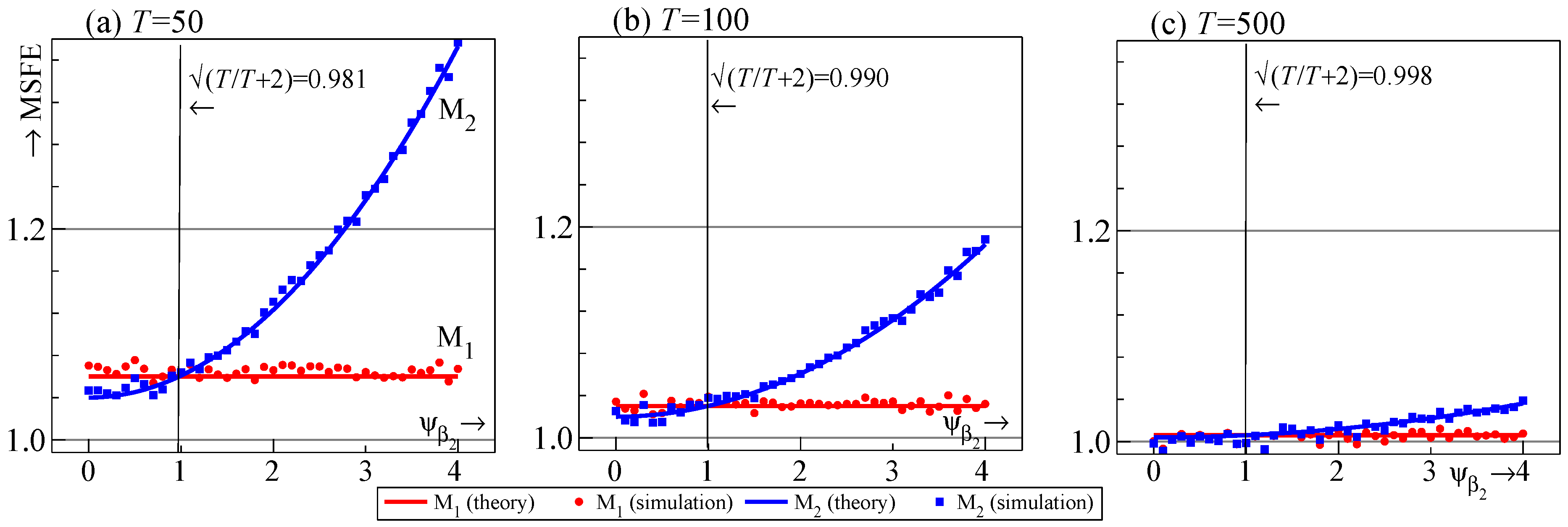
Figure 2 records the one-step-ahead values of ${\mathrm{MSFE}}_1$ and ${\mathrm{MSFE}}_2$ for known $x_{i,T+1},i=1,2$, for the DGP given by (1) and (2). We let ${\beta }_2$ vary along the horizontal axis to get a range of noncentralities in the set ${\psi }_{\beta }=\left[0,4\right]$ using (7).

The results confirm that $x_2$ should be retained if its noncentrality exceeds approximately 1. The result converges to 1 as $T\to \infty$, because the information content of the regressor outweighs the parameter estimation cost for one-step forecasts, regardless of the correlation between $x_1$ and $x_2$.

4.2. Selecting Regressors

Although ${\mathrm{M}}_1$ and ${\mathrm{M}}_2$ provide the extremes of always/never retaining $x_2$, in practice, selection will be applied. From (5), $x_{2,t}$ will be omitted if ${\mathrm{t}}_{{\beta }_2=0}^2<c_{\alpha }^2$. Using the approximation that:

$${\mathrm{t}}_{{\beta }_2=0}=\frac{{\widehat{\beta }}_2}{s.e.\left[{\widehat{\beta }}_2\right]}\approx \frac{\sqrt{T\left(1-{\rho }^2\right)}{\widehat{\beta }}_2}{{\sigma }_{ϵ}},$$

implies:

$${\widehat{\beta }}_2^2<\frac{c_{\alpha }^2{\sigma }_{ϵ}^2}{T\left(1-{\rho }^2\right)}.$$

(11)

Thus, retention of $x_{2,t}$ will depend on $\alpha$ and ${\psi }_{\beta }^2$ for a given draw.

Forecasts in repeated sampling will be based on a mixture of ${\mathrm{M}}_1$ and ${\mathrm{M}}_2$ depending on whether $x_{2,t}$ is retained in each draw. The MSFE of the selected model, called ${\mathrm{M}}_3$, will be a weighted average of the MSFEs of ${\mathrm{M}}_1$ and ${\mathrm{M}}_2$, with the weights given by the probability that $x_{2,t}$ is retained:

$$\begin{array}{cc}\hfill {\mathrm{MSFE}}_3& ={\mathrm{p}}_{\alpha }\left({\psi }_{\beta }\right){\mathrm{MSFE}}_1+\left(1-{\mathrm{p}}_{\alpha }\left({\psi }_{\beta }\right)\right){\mathrm{MSFE}}_2\hfill \end{array}$$

$$\begin{array}{cc}\hfill & ={\mathrm{MSFE}}_1+\left(1-{\mathrm{p}}_{\alpha }\left({\psi }_{\beta }\right)\right)\left({\mathrm{MSFE}}_2-{\mathrm{MSFE}}_1\right)\hfill \end{array}$$

(12)

$$\begin{array}{cc}\hfill & \approx {\mathrm{MSFE}}_1+{\sigma }_{ϵ}^2{T}^{-1}\left(1-{\mathrm{p}}_{\alpha }\left({\psi }_{\beta }\right)\right)\left({\psi }_{\beta }^2-1\right),\hfill \end{array}$$

(13)

where ${\psi }_{\beta }^2$ is given by (7), with:

$${\mathrm{p}}_{\alpha }\left({\psi }_{\beta }\right)=Pr\left({\mathrm{t}}_{{\beta }_2=0}^2\geqq c_{\alpha }^2\right).$$

From the last term in (13), it is clear that ${\mathrm{MSFE}}_3\le {\mathrm{MSFE}}_1$ whenever ${\psi }_{\beta }^2\le 1$. Moreover, ${\mathrm{p}}_{\alpha }\left({\psi }_{\beta }\right)$ will be low when ${\psi }_{\beta }^2\le 1$, so ${\mathrm{M}}_2$ will usually be selected. Note that ${\mathrm{p}}_{\alpha }\left({\psi }_{\beta }\right)=\alpha$ when ${\beta }_2=0$. However, ${\mathrm{MSFE}}_3$ is a highly nonlinear function of ${\psi }_{\beta }^2$ entering directly and indirectly, as well as of $\alpha$ which also influences ${\mathrm{p}}_{\alpha }\left({\psi }_{\beta }\right)$ nonlinearly.

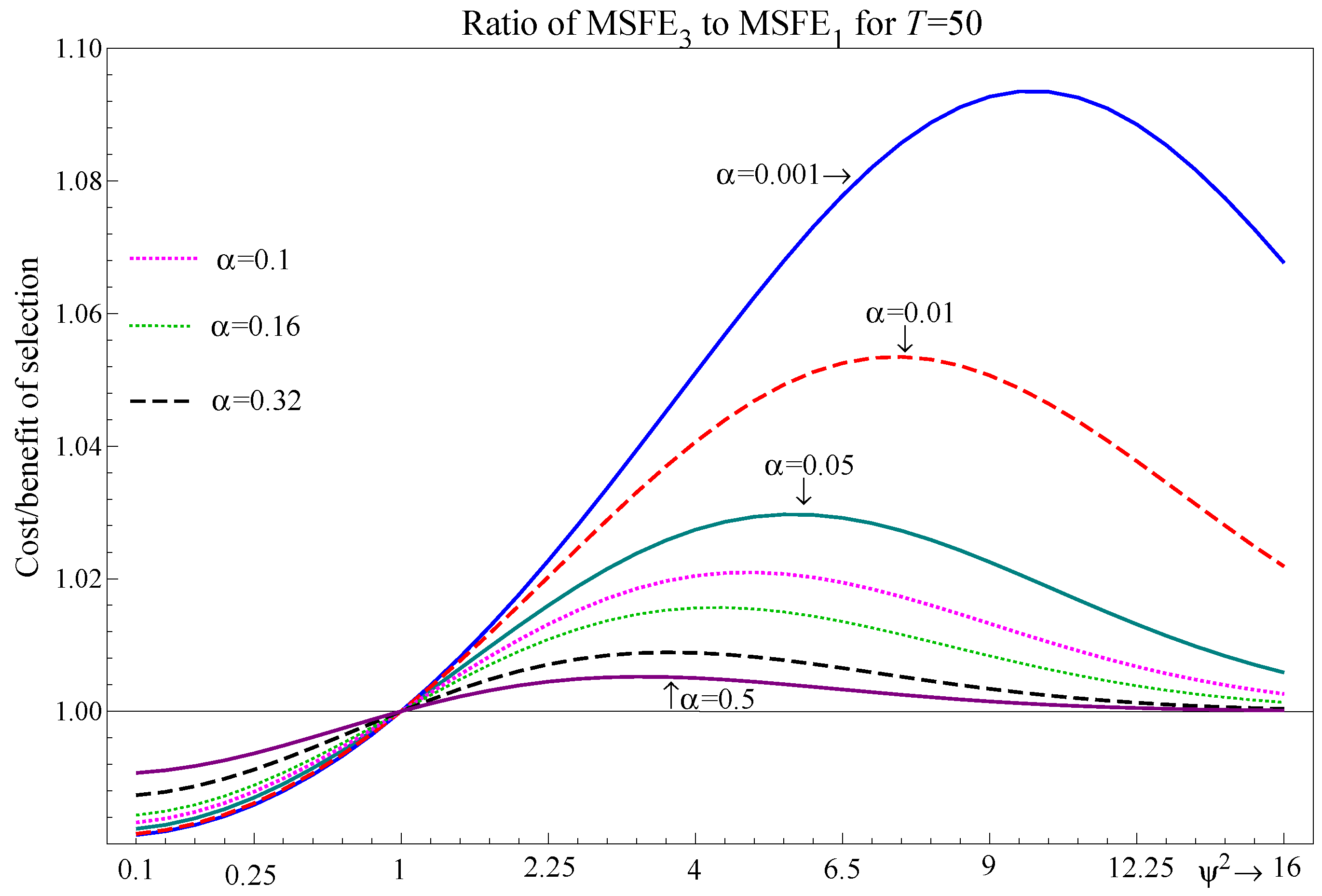
Figure 3 records the ratio of ${\mathrm{MSFE}}_3$ to ${\mathrm{MSFE}}_1$, for a range of ${\psi }_{\beta }^2$, which from (13) is given by:

$$\frac{{\mathrm{MSFE}}_3}{{\mathrm{MSFE}}_1}\approx 1+{\left(T+3\right)}^{-1}\left(1-{\mathrm{p}}_{\alpha }\left({\psi }_{\beta }\right)\right)\left({\psi }_{\beta }^2-1\right).$$

(14)

Selection delivers a 1.8% improvement in MSFE relative to ${\mathrm{M}}_1$ under the null when ${\psi }_{\beta }^2=0$ with $\alpha =0.05$ or tighter, but for looser $\alpha$, e.g., at 0.5, ${\mathrm{p}}_{\alpha }\left({\psi }_{\beta }\right)=0.5$ when $x_{2,t}$ is irrelevant so the benefits of selection are halved. Selection is most costly at intermediate noncentralities under the alternative, where, e.g., the largest increase in MSFE relative to ${\mathrm{M}}_1$ is 3% at $\alpha =0.05$ for $T=50$, but is over 9% for $\alpha =0.001$ at its peak. The hump shape reflects the nonlinear trade-off as the noncentrality of $x_{2,t}$ increases from the cost of omitting $x_{2,t}$ rising as its signal is stronger, but the probability of retaining $x_{2,t}$ also increases. While the magnitude of the maximal loss may seem small for intermediate values of $\alpha$, this example considers the selection of just one regressor. In practice, selection is applied when there are multiple potential regressors, and the loss associated with selection at a given significance level is cumulated across all potential regressors, as seen in the simulation results below.

The selection rule that $x_{2,t}$ should be retained if ${\psi }_{\beta }^2>1$ is evident $\forall \alpha$, but unfortunately the forecaster does not know ${\psi }_{\beta }^2$. If it was known, the optimal $\alpha$ is 0 for ${\psi }_{\beta }^2<1$ and 1 for ${\psi }_{\beta }^2>1$. We next look at the choice of $\alpha$ to minimize cost in terms of improvements in MSFEs for an unknown ${\psi }_{\beta }^2$.

4.3. The Choice of Significance Level

Equation (11) must hold for $x_2$ to be excluded at the chosen significance level. On average, that inequality requires:

$$\mathrm{E}\left[{\widehat{\beta }}_2^2\right]=\mathrm{V}\left[{\widehat{\beta }}_2\right]+{\beta }_2^2={\beta }_2^2+\frac{{\sigma }_{ϵ}^2}{T\left(1-{\rho }^2\right)}<\frac{c_{\alpha }^2{\sigma }_{ϵ}^2}{T\left(1-{\rho }^2\right)},$$

assuming unbiasedness. Equating that inequality for ${\beta }_2^2$ with ${\psi }_{\beta }^2<1$ from (10) gives the boundary for the critical value $c_{\alpha }$ in which selection results in a smaller MSFE due to the omission–estimation trade-off:

$${\beta }_2^2=\frac{{\sigma }_{ϵ}^2\left(c_{\alpha }^2-1\right)}{T\left(1-{\rho }^2\right)}\le \frac{{\sigma }_{ϵ}^2}{T\left(1-{\rho }^2\right)}.$$

This implies that $c_{\alpha }^2=2$ at the boundary, or an approximate significance level of $\alpha =0.16$.

The theoretical probability of retaining $x_2$ for ${\beta }_2>0$ at $\alpha =0.16$ using $\mathrm{E}\left[{\mathrm{t}}_{{\widehat{\beta }}_2}\right]={\psi }_{\beta }$ is:

$$Pr\left({\mathrm{t}}_{{\widehat{\beta }}_2}\geqq c_{\alpha }\right)=Pr\left({\mathrm{t}}_{{\widehat{\beta }}_2}-{\psi }_{\beta }\geqq c_{\alpha }-{\psi }_{\beta }\right).$$

This gives the retention probabilities recorded in

Table 2. Retention probabilities for individual t-tests given $\mathrm{E}\left[{\mathrm{t}}_{{\widehat{\beta }}_2}\right]={\psi }_{\beta }$.

${\mathit{\psi }}_{\mathit{\beta }}$	1	2	3	4
${\mathrm{P}}_{0.16}$	0.34	0.72	0.94	0.995
${\mathrm{P}}_{0.05}$	0.16	0.51	0.85	0.98

.

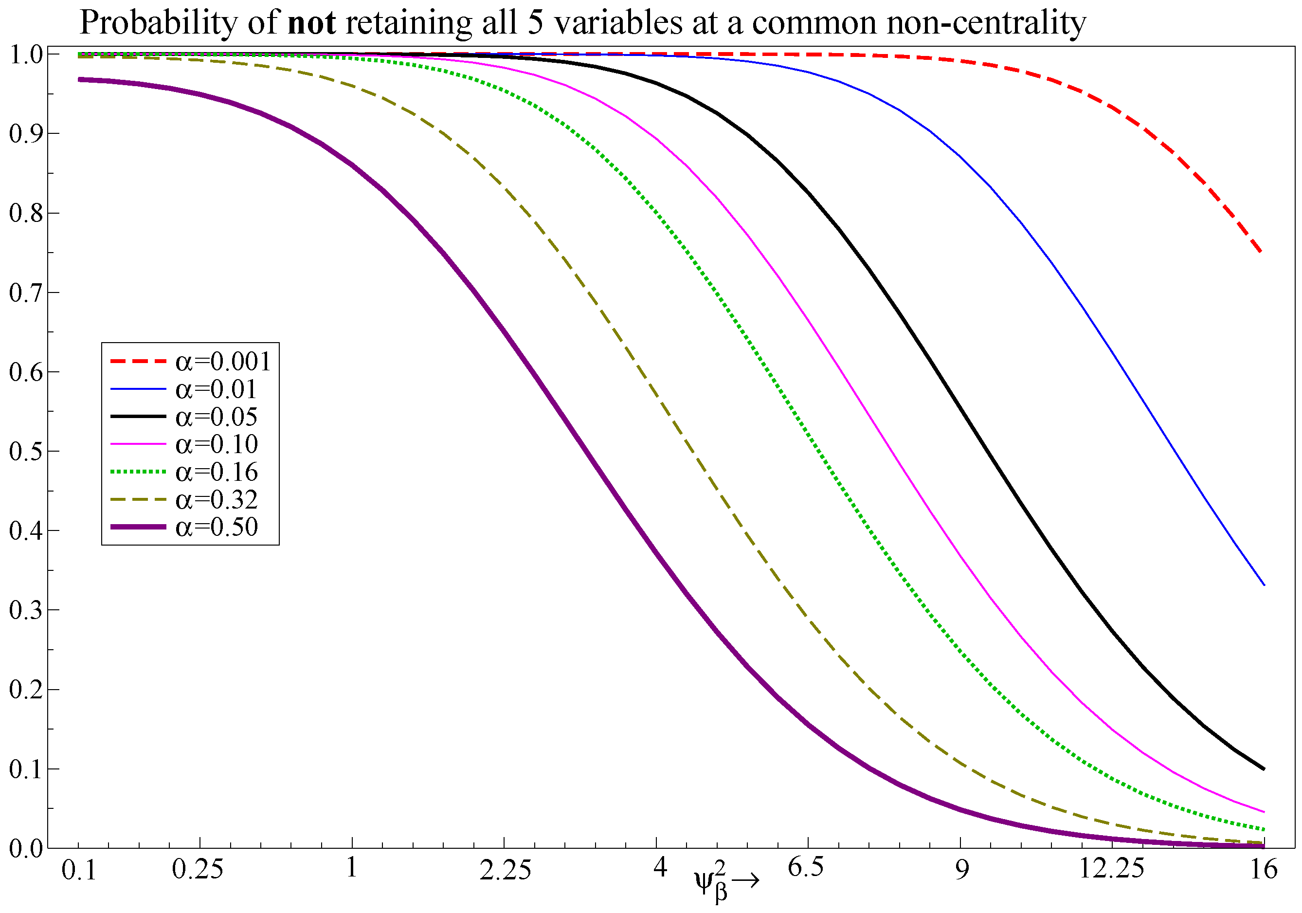
These results are close to the implied significance level for the AIC in Campos et al. (2003). This can have a cumulative effect, as shown in Figure 4 which records values of the term $\left(1-{\mathrm{p}}_{\alpha }\left({\psi }_{\beta }\right)\right)$ where there are five independent regressors, all with the same ${\psi }_{\beta }^2$. The probability of retaining all five variables is low even at loose significance levels unless the noncentralities are large. At ${\psi }_{\beta }^2=9$ the gap between $\alpha =0.05$ and $\alpha =0.16$ is 29%, demonstrating large benefits to a looser significance level for the retention of relevant regressors. The trade-off is that more irrelevant variables will be retained, and this can be costly if those variables are subject to breaks, which we next explore.

5. An Out-of-Sample Shift in the Regressors

The analysis of the previous section is augmented by the introduction of a break in Section 5.1. This break is immediately after the estimation sample, while in Section 6 it is applied to the last in-sample observation. We distinguish between whether the future values of the regressors are known (Section 5.2) or unknown (Section 5.4). The role of selection is studied again (Section 5.3), and we look at the random walk as a device to forecast future values of the regressors in Section 5.5. Forecasting devices based on full in-sample information and a random walk are the extremes of the class in Castle et al. (2015), but there is no information in sample regarding the break to help either device.

5.1. Specification of the Out-of-Sample Shift

Consider a mean shift of size $\delta$ in $x_2$ at $T+1$ with the forecast origin at T, so the shift coincides with the one-step-ahead forecast. The DGP has the same structure as (1)–(3) with the parameters $\left({\beta }_1{\beta }_2\right)$ of the conditional model constant:

$$\begin{array}{cc}\hfill x_{1,t}& ={\mu }_1+{\eta }_{1,t}t=1,\dots ,T+1,\hfill \\ \hfill x_{2,t}& =\left\{\begin{array}{c}{\mu }_2+{\eta }_{2,t}t=1,\dots ,T,\hfill \\ {\mu }_2+\delta +{\eta }_{2,t}t=T+1.\hfill \end{array}\right.\hfill \end{array}$$

(15)

Since (15) entails:

$$\begin{array}{cc}\hfill y_{T+1}& ={\beta }_0+{\beta }_1{x}_{1,T+1}+{\beta }_2{x}_{2,T+1}+{ϵ}_{T+1}\hfill \\ \hfill & =\left({\mu }_y+{\beta }_2\delta \right)+{\beta }_1\left(x_{1,T+1}-{\mu }_1\right)+{\beta }_2\left(x_{2,T+1}-{\mu }_2-\delta \right)+{ϵ}_{T+1},\hfill \end{array}$$

(16)

then ${\beta }_2\delta \ne 0$ induces a location shift in the relationship between $y_{T+1}$ and its in-sample determinants unless the future $x_{2,T+1}$ is known at time T. As shown in all forecast-error taxonomies (see e.g., Clements and Hendry 1998), shifts in the equilibrium mean are the most pernicious source of forecast failure, whereas changes in the parameters of mean-zero variables have only a variance impact. Omitting $x_{2,T+1}$ from (16) as in ${\mathrm{M}}_2$ will create the same location shift. Thus, there is little loss of generality by only considering shifts in the regressors.

We first evaluate the trade-off to omitting $x_{2,t}$ for known future exogenous regressors, emulating the above results as the break which occurs in the forecast period is modeled in the known $x_{2,T+1}$.

5.2. Known Future Values of Regressors

The one-step-ahead forecasts for ${\mathrm{M}}_1$ given (15), in which values of ${\mathbf{x}}_{T+1}$ are assumed to be known at T, are unbiased when the parameter estimates are unbiased. The mean square forecast error of ${\mathrm{M}}_1$ (see Appendix A.3 for derivations) is:

$${\mathrm{MSFE}}_1=\mathrm{E}\left[{\overline{\widehat{ϵ}}}_{T+1|T+1}^2\right]={\sigma }_{ϵ}^2\left(1+\frac{1}{T\left(1-{\rho }^2\right)}\left({\delta }^2+2-\rho \right)\right),$$

(17)

which does not depend on ${\psi }_{\beta }^2$. Comparison with (8) highlights the effects of the location shift: ${\delta }^2$ enters the MSFE despite the shift being ‘known’ given $x_{2,T+1}$, and ${\mathrm{MSFE}}_1$ is no longer independent of $\rho$. (17) also reveals the additional costs of including an irrelevant regressor which shifts out of sample as ${\delta }^2$ enters even when ${\beta }_2=0$, although it is scaled by $T\left(1-{\rho }^2\right)$ so larger samples mitigate its effect.

For ${\mathrm{M}}_2$ (which omits the regressor $x_{2,t}$), the expectation of the forecast error is $\mathrm{E}\left[{\overline{\widetilde{ϵ}}}_{T+1|T+1}\right]={\beta }_2\delta$, so the forecasts are biased by the shift in the omitted variable. The one-step-ahead MSFE for ${\mathrm{M}}_2$ is:

$${\mathrm{MSFE}}_2=\mathrm{E}\left[{\overline{\widetilde{ϵ}}}_{T+1|T+1}^2\right]={\sigma }_{ϵ}^2+{\beta }_2^2\left(1-{\rho }^2+{\delta }^2\right)+2T^{-1}{\sigma }_{ϵ}^2\left(1+T^{-1}{\psi }_{\beta }^2\right),$$

(18)

where ${\beta }_2^2$ enters directly so the MSFE is a function of ${\psi }_{\beta }^2$, unlike for ${\mathrm{M}}_1$. Comparison with (9) reveals the role that $\rho$ and ${\delta }^2$ play. When ${\beta }_2=0$, so ${\mathrm{M}}_2$ is the correct model, (18) collapses to (9).

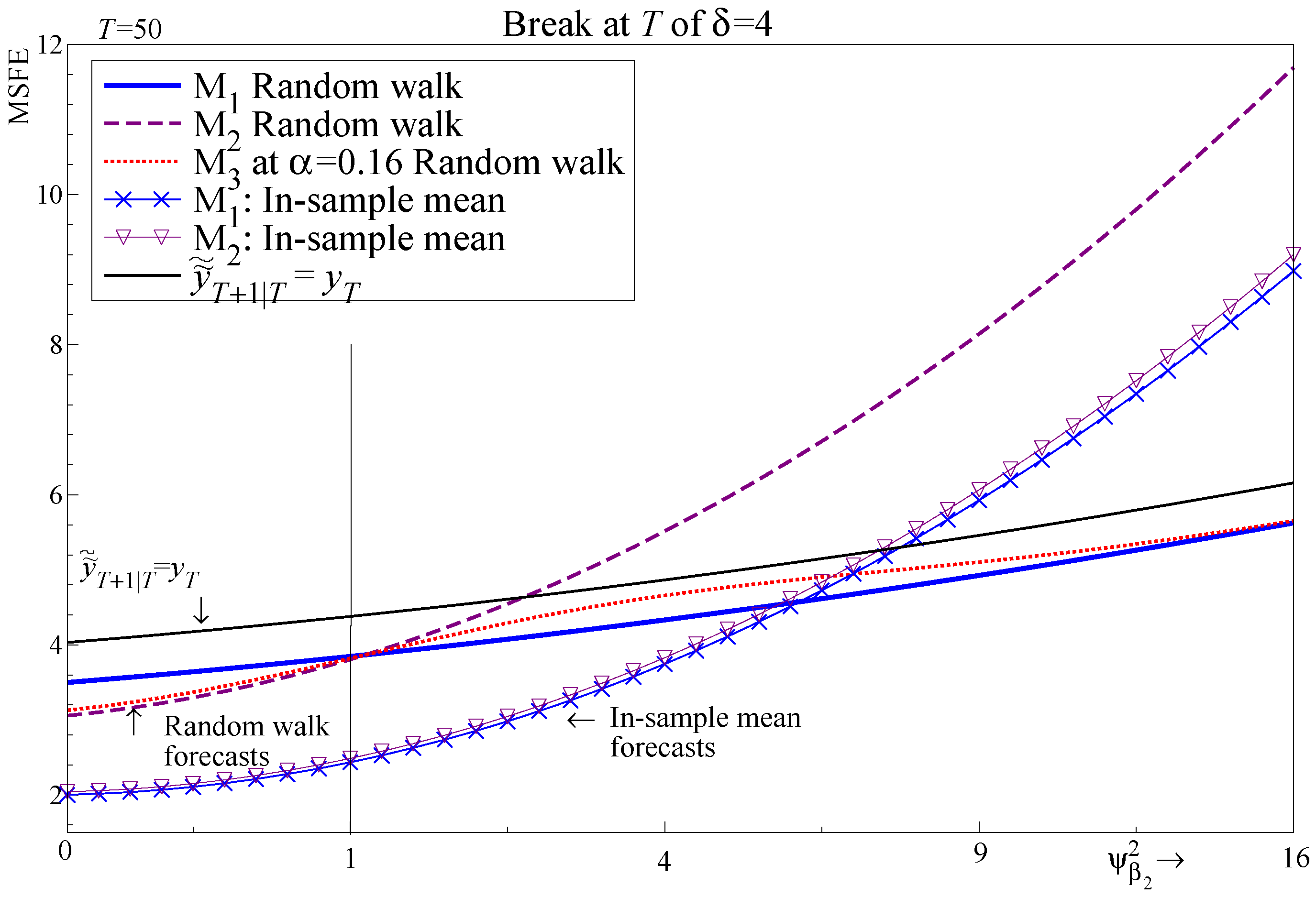
Assuming a criterion of minimizing one-step-ahead MSFE, using (10), ${\mathrm{MSFE}}_2\le {\mathrm{MSFE}}_1$ requires:

$${\delta }^2\left({\psi }_{\beta }^2-1\right)+{\psi }_{\beta }^2\left(1-{\rho }^2\right)\left(1+2T^{-1}\right)-\rho <0,$$

(19)

which depends on estimation uncertainty and therefore does not simplify neatly. However, the solution is close to 1 for reasonable values of $\rho$. For example, when $\rho =0.5$, $T=50$ and $\delta =4$, then ${\psi }_{\beta }^2<0.983$, or $|{\psi }_{\beta }|<0.991$, results in a smaller ${\mathrm{MSFE}}_2$ compared to ${\mathrm{MSFE}}_1$.

Figure 5 demonstrates the close approximation to a trade-off at ${\psi }_{\beta }=1$ which holds regardless of the break. Thus, even knowing there is a shift in $x_2$ does not affect the choice of forecasting model between including or omitting $x_2$: always (never) include for ${\psi }_{\beta }^2\ge 1$ (${\psi }_{\beta }^2<1$).

5.3. Selecting Regressors

Following Section 4.2, a t-test for statistical significance will be conducted on $x_{2,t}$ in sample and a decision to retain or exclude $x_{2,t}$ will be made at $c_{\alpha }$ for a given draw. Hence, ${\mathrm{MSFE}}_3$ will be a weighted average of ${\mathrm{MSFE}}_1$ and ${\mathrm{MSFE}}_2$, using (12):

$${\mathrm{MSFE}}_3={\mathrm{MSFE}}_1+\left(1-{\mathrm{p}}_{\alpha }\left({\psi }_{\beta }\right)\right)\left({\sigma }_{ϵ}^2{T}^{-1}\left[{\psi }_{\beta }^2\left\{1+\frac{{\delta }^2}{\left(1-{\rho }^2\right)}\right\}-\frac{{\delta }^2+2-\rho }{\left(1-{\rho }^2\right)}\right]\right).$$

(20)

The term in square brackets is scaled by $T^{-1}$. As before, the difference between ${\mathrm{MSFE}}_1$ and ${\mathrm{MSFE}}_3$ diminishes as the sample size increases. When ${\psi }_{\beta }^2=0$, the first term in square brackets in (20) drops out and the benefits of selection relative to ${\mathrm{MSFE}}_1$ are evident as the second term must be negative. The magnitude of ${\delta }^2$ affects both ${\mathrm{MSFE}}_1$ and ${\mathrm{MSFE}}_2$ but, from (20), the first ${\delta }^2$ term is multiplied by ${\psi }_{\beta }^2$ whereas the second offsetting term is not, so the effect of the location shift is exacerbated if ${\psi }_{\beta }^2>1$.

Figure 5 compares the MSFEs of ${\mathrm{M}}_1$ from (17), ${\mathrm{M}}_2$ from (18), and ${\mathrm{M}}_3$ using (20) at three illustrative values of $\alpha$. The profiles of the MSFEs mirror the analytical results for the no break case. Selection outperforms the estimated DGP for ${\psi }_{\beta }^2<1$ despite a break, and remains close to the ${\mathrm{MSFE}}_1$ at $\alpha =0.16$ for ${\psi }_{\beta }^2>1$.

5.4. Unknown Future Values of Regressors

Now consider when the future values of the regressors are unknown. We use two devices to obtain forecasts of $x_{i,T+1}$, $i=1,2$: the in-sample mean or a random walk. The random walk is biased for unanticipated location shifts but does not result in systematic bias following a location shift, whereas the in-sample mean is persistently biased following a location shift unless updated. The two devices comprise the two extremes of using either the full in-sample data or only the last observation to produce the forecasts of the weakly exogenous regressors.3

Although the link between y and the $x_i$ stays constant, forecasts when the $x_{i,T+1}$ are unknown will fail if the shift at $T+1$ is not anticipated, inducing a shift in $y_{T+1}$. This will lead to forecast failure as the in-sample mean ${\mu }_y$ shifts to $({\mu }_y+{\beta }_2\delta )$ at $T+1$ but would be forecast to be ${\mu }_y$.

The forecasts based on in-sample estimates from (15) when ${\mu }_1$ and ${\mu }_2$ are not zero are given by:

$$\begin{array}{cc}\hfill {\overline{x}}_{1,T+1|T}& ={\widehat{\mu }}_1=\frac{1}{T}{\sum }_{t=1}^T{x}_{1,t}={\mu }_1+{\overline{\eta }}_1,\hfill \end{array}$$

(21)

$$\begin{array}{cc}\hfill {\overline{x}}_{2,T+1|T}& ={\widehat{\mu }}_2=\frac{1}{T}{\sum }_{t=1}^T{x}_{2,t}={\mu }_2+{\overline{\eta }}_2,\hfill \end{array}$$

(22)

so will miss the unknown break. When the break occurs in $x_2$, the MSFEs will worsen for ${\beta }_2\ne 0$. As before, we consider the sampling variation in estimating the means as small compared to the impact of shifts, so we approximate by taking T sufficiently large that ${\widehat{\mu }}_i\approx {\mu }_i$.

Replacing the unknown $x_{i,T+1}$ by ${\mu }_i$ leads to forecasting $y_{T+1}$ by the in-sample mean for both ${\mathrm{M}}_1$ and ${\mathrm{M}}_2$, see Appendix A.4. Both face the same forecast bias, $\mathrm{E}\left[{\widehat{\widehat{ϵ}}}_{T+1|T}\right]=\mathrm{E}\left[{\widetilde{\tilde{ϵ}}}_{T+1|T}\right]={\beta }_2\delta$ which is the same bias as ${\mathrm{M}}_2$ with known regressors. Parameter estimation adds terms of ${\mathrm{O}}_p\left(T^{-1}\right)$. Hence, ignoring ${\mathrm{O}}_p\left(T^{-1}\right)$ terms, ${\mathrm{MSFE}}_1={\mathrm{MSFE}}_2$:

$$\mathrm{E}\left[{\widehat{\widehat{ϵ}}}_{T+1|T}^2\right]=\mathrm{E}\left[{\widetilde{\tilde{ϵ}}}_{T+1|T}^2\right]={\beta }_2^2{\delta }^2+{\sigma }_{ϵ}^2+\left({\beta }_1^2+{\beta }_2^2+2\rho {\beta }_1{\beta }_2\right).$$

(23)

When ${\beta }_2=0$, the MSFE is ${\sigma }_{ϵ}^2+{\beta }_1^2$, so is inflated relative to the known regressors case as $x_{1,T+1}$ must also be forecast. However, the in-sample mean forecast is the best forecast device for $x_{1,T+1}$ in this setting (in terms of minimum MSFE) as $x_{1,T+1}$ is stationary and not subject to a location shift. Selection will have little or no noticeable impact when ${\mathrm{MSFE}}_2\approx {\mathrm{MSFE}}_1$, as this will also result in ${\mathrm{MSFE}}_3\approx {\mathrm{MSFE}}_1$.

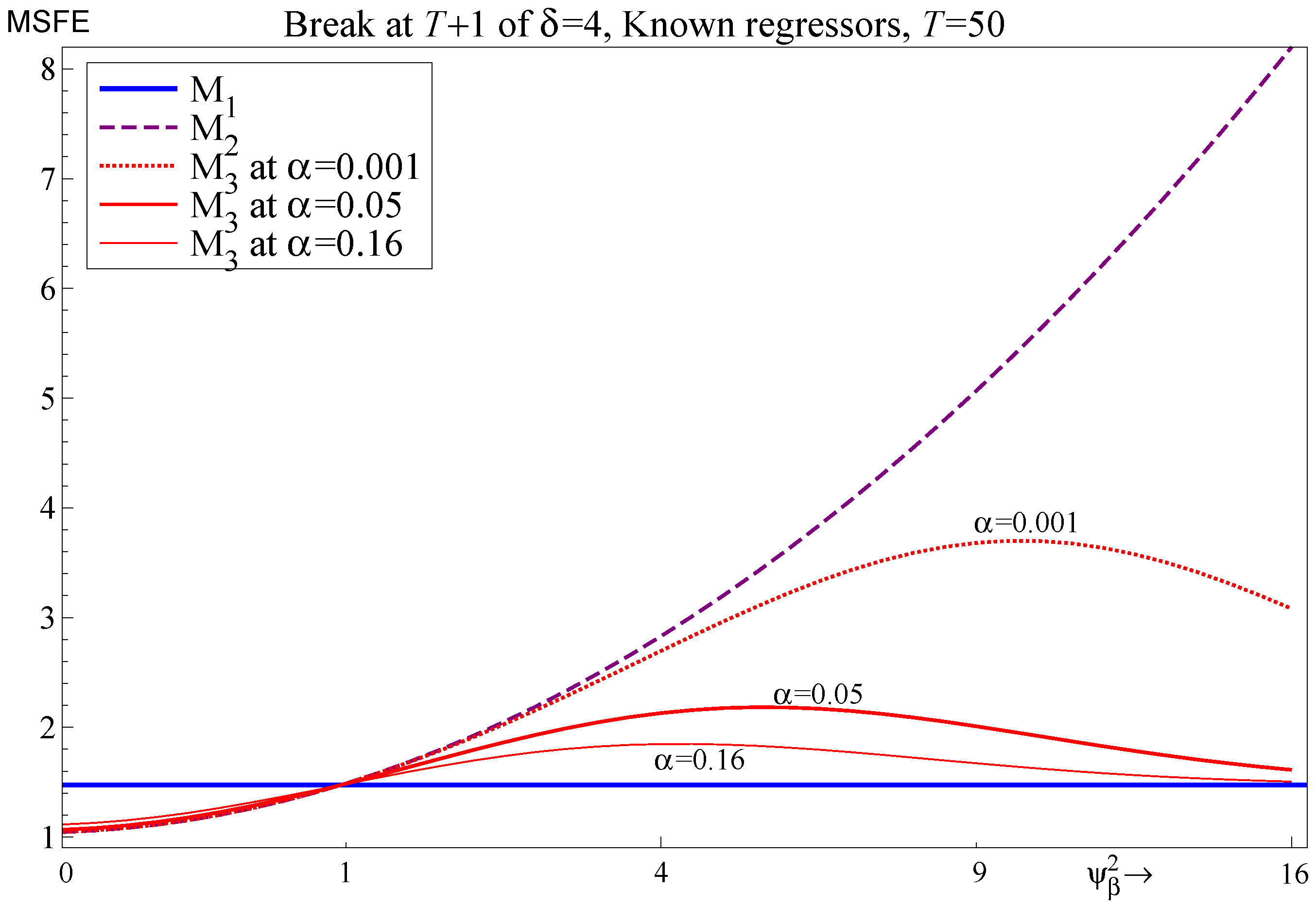
Figure 6 records the MSFEs for ${\mathrm{M}}_1$ and ${\mathrm{M}}_2$ when there is a break in $x_2$ at $T+1$, comparing known and unknown regressors using the in-sample mean to forecast $x_{i,T+1}$, $i=1,2$ in the unknown regressor case, i.e., the figure records (17), (18) and (23), (solid/dashed/dotted lines). Simulation outcomes are checked to capture ${\mathrm{O}}_p\left(T^{-1}\right)$ effects but they are negligible so are not recorded. Figure 6 includes the random walk forecasts and the ${\mathrm{M}}_1$ and ${\mathrm{M}}_2$ results for the known regressor case are repeated from Figure 5 to facilitate comparison.

The simulation outcomes where parameters are estimated closely match the analytic results. For known regressors for ${\mathrm{MSFE}}_1$, the break in ${\mu }_2$ does not affect the MSFE as it is captured in $x_{2,T+1}$: even at $\delta =4$ for $T=100$, ${\mathrm{MSFE}}_1=1.23$ for the parameters given in the figure which is only slightly greater than ${\sigma }_{ϵ}^2$. However, when ${\mathbf{x}}_{T+1}$ is unknown both ${\mathrm{M}}_1$ and ${\mathrm{M}}_2$ are affected by the break in $x_{2,T+1}$. Simulation outcomes again closely match the theory for the unknown break case, and show that the choice of whether to retain or exclude $x_{2,t}$ is not important in a forecasting context. The unanticipated break dominates any forecast error resulting from model misspecification. Increasing the sample size does mitigate the MSFE costs but the MSFE premium relative to known regressors is maintained for all ${\psi }_{\beta }^2$. Increasing the number of relevant exogenous regressors that shift will increase the MSFE at ${\psi }_{\beta }^2=0$, shifting the MSFE trajectories up.

These results show that in this static setting of location shifts, if the break occurs in the forecast period and is unknown and unpredictable, then the retention of $x_2$ is irrelevant (other than parameter estimation uncertainty), as neither ${\mathrm{M}}_1$ nor ${\mathrm{M}}_2$ capture the shift which dominates the MSFE. Parsimony, or lack thereof, neither helps nor hinders much in this setting. Moreover, selection does not substantively affect the outcome as ${\mathrm{MSFE}}_3\approx {\mathrm{MSFE}}_1$.

5.5. Forecasting Regressors with a Random Walk

We now consider using a random walk to forecast the exogenous variables:

$$\begin{array}{cc}\hfill {\overline{\overline{x}}}_{1,T+1|T}& =x_{1,T},\hfill \end{array}$$

(24)

$$\begin{array}{cc}\hfill {\overline{\overline{x}}}_{2,T+1|T}& =x_{2,T}.\hfill \end{array}$$

(25)

Such a device is not robust in this setting as the forecasts are made before the shift, and robustness refers to forecasting properties that are insensitive to a feature in the DGP, such as after a location shift.

Although the last in-sample observation is an imprecise measure of the out-of-sample mean, it is unbiased when there are no location shifts (as there are no dynamics in the DGP), so $\mathrm{E}\left[x_{1,T}\right]={\mu }_1$ and $\mathrm{E}\left[x_{2,T}\right]={\mu }_2$, and hence $\mathrm{E}\left[\Delta x_{1,T+1}\right]=0$ and $\mathrm{E}\left[\Delta x_{2,T+1}\right]=\delta$.

The forecasts from ${\mathrm{M}}_1$ will be biased by the bias in the random walk forecast of $x_{2,T+1}$, so (see Appendix A.5 for derivations) neglecting the small impact of ${\eta }_{i,T}$ on ${\beta }_i-{\widehat{\beta }}_i$:

$$\mathrm{E}\left[{\overline{\overline{ϵ}}}_{T+1|T}\right]={\beta }_2\delta ,$$

and the resulting mean square forecast error is:

$${\mathrm{MSFE}}_1=\mathrm{E}\left[{\overline{\overline{ϵ}}}_{T+1|T}^2\right]={\beta }_2^2{\delta }^2+2\left({\beta }_1^2+{\beta }_2^2\right)+4\rho {\beta }_1{\beta }_2+{\sigma }_{ϵ}^2\left(1+2T^{-1}\right).$$

(26)

Comparison with (23) highlights the additional cost of using the random walk relative to the in-sample mean when neither forecasting device can predict the break, since:

$$\mathrm{E}\left[{\widehat{\widehat{ϵ}}}_{T+1|T}^2\right]-\mathrm{E}\left[{\overline{\overline{ϵ}}}_{T+1|T}^2\right]=-\left({\beta }_1^2+{\beta }_2^2+2\rho {\beta }_1{\beta }_2+2{\sigma }_{ϵ}^2{T}^{-1}\right).$$

The in-sample mean of $x_1$ is the optimal forecast of $x_{1,T+1}$ given its in-sample stationarity, so irrespective of the value of ${\beta }_2$, the in-sample mean forecasts dominate when the shift is during the forecast period. When ${\beta }_2=0$, (26) collapses to $\approx {\sigma }_{ϵ}^2+2{\beta }_1^2$, ignoring ${\mathrm{O}}_p\left(T^{-1}\right)$ terms, compared to ${\sigma }_{ϵ}^2+{\beta }_1^2$ for the in-sample mean forecasts. A random walk doubles the error variance, so can be costly if there are no breaks or if the break occurs after the forecast origin. As for the in-sample mean case, the MSFE of ${\mathrm{M}}_1$ is a function of the break.

The forecast bias for ${\mathrm{M}}_2$ is the same as that for ${\mathrm{M}}_1$ by the same argument, although ${\mathrm{MSFE}}_2$ (reported in Appendix A.5) does deviate from that for ${\mathrm{M}}_1$ as ${\psi }_{\beta }^2$ increases. This is due to the correlation parameter $\rho$ which is picking up part of the omitted variable $x_{2,T+1}$ in ${\mathrm{M}}_2$ and has more effect as ${\psi }_{\beta }^2$ increases. When ${\beta }_2=0$, ${\mathrm{MSFE}}_2\approx {\sigma }_{ϵ}^2+2{\beta }_1^2$, which is the same as for ${\mathrm{M}}_1$. Despite small but increasing deviations as ${\psi }_{\beta }^2$ increases, ${\mathrm{MSFE}}_2$ follows a similar trajectory to ${\mathrm{MSFE}}_1$. The misspecification is less relevant for the random walk forecasts of the marginal processes relative to the effect of the break, similar to the results for the in-sample mean forecasts.

5.6. Selecting Forecasted Regressors

In practice, selection will be applied to determine whether to include $x_{2,t}$ or not. Then, from (12), we can obtain the ${\mathrm{MSFE}}_3$ as:

$$\begin{array}{cc}\hfill {\mathrm{MSFE}}_3& ={\mathrm{MSFE}}_1+\left(1-{\mathrm{p}}_{\alpha }\left({\psi }_{\beta }\right)\right)\left({\sigma }_{ϵ}^2{T}^{-1}\left[{\psi }_{\beta }^2\left\{\frac{\left(1+{\rho }^2\right)}{\left(1-{\rho }^2\right)}+T^{-1}\right\}+1\right]\right).\hfill \end{array}$$

The trade-off between parameter estimation uncertainty and including $x_2$ is essentially the same as in the known variable case: if $x_2$ has a noncentrality of zero, so ${\beta }_2={\psi }_{\beta }^2=0$, then the one-step MSFE is minimized by excluding $x_2$ from the forecasting model. It should be included if ${\psi }_{\beta }^2>1$. However, depending on the values of $\rho$ and T, the switch point can be smaller than ${\psi }_{\beta }^2=1$, although the impact is likely to be small given the scale factor ${\sigma }_{ϵ}^2{T}^{-1}$. Even though the random walk forecast is highly uncertain by using just one observation, if the variable that breaks is quite significant then it pays to include that variable when using the random walk forecast.

Figure 6 also records the MSFEs for the random walk forecasts using the same parameter values. The increase in MSFE over the in-sample mean forecasts is evident. Both ${\mathrm{MSFE}}_1$ and ${\mathrm{MSFE}}_2$ follow similar trajectories, although they do start to diverge for large ${\psi }_{\beta }^2$, with ${\mathrm{MSFE}}_3$ at $\alpha =0.16$ close to ${\mathrm{MSFE}}_1$.

6. An In-Sample Shift in the Regressors

In contrast to the previous section, the break is assumed to occur at T, which is the last observation available for estimation. Now there is information available regarding the break when the forecasts are made. Such a framework would also be relevant in sequential forecasting. We consider forecasting using in-sample means. In common with the previous section, we study selection (Section 6.3 and Section 6.5), the random walk device to forecast the regressors (Section 6.4), and finally using the random walk to forecast y (Section 6.6).

6.1. Specification of the In-Sample Shift

The DGP is adapted from (15) but the shift in ${\mu }_2$ occurs at T, rather than $T+1$:

$$\begin{array}{cc}\hfill x_{1,t}& ={\mu }_1+{\eta }_{1,t}t=1,\dots ,T+1,\hfill \\ \hfill x_{2,t}& =\left\{\begin{array}{c}{\mu }_2+{\eta }_{2,t}t=1,\dots ,T-1,\hfill \\ {\mu }_2+\delta +{\eta }_{2,t}t=T,T+1.\hfill \end{array}\right.\hfill \end{array}$$

(27)

6.2. Forecasting Regressors Using In-Sample Means

The relationship of interest, i.e., the conditional equation for $y_{T+1}$, remains constant. However, the in-sample mean ${\mu }_y$ is shifted to $({\mu }_y+{\beta }_2\delta )$ at T. Although the only DGP parameter to shift is ${\mu }_2$ to ${\mu }_2+\delta$, sample calculations will be altered as now $\mathrm{E}\left[{\overline{x}}_2\right]={\mu }_2+T^{-1}\delta$ (see Appendix A.6 for derivations).

The impact on the estimated in-sample mean of $\left\{x_{2,t}\right\}$ will be small from the break, unless $\delta$ is very large, so by using the in-sample means for their future unknown values, the forecasted mean of $y_{T+1}$ for ${\mathrm{M}}_1$ will still be close to ${\mu }_y$, and the resulting forecast error bias is:

$$\mathrm{E}\left[{\widehat{\widehat{ϵ}}}_{T+1|T+1}\right]\approx {\beta }_2\delta \left(1-T^{-1}\right).$$

This is unbiased when ${\beta }_2=0$, but could be badly biased if ${\beta }_2\delta$ is large. The MSFE for ${\mathrm{M}}_1$ is:

$${\mathrm{MSFE}}_1=\mathrm{E}\left[{\widehat{\widehat{ϵ}}}_{T+1|T+1}^2\right]={\beta }_2^2{\delta }^2{\left(1-T^{-1}\right)}^2+{\beta }_1^2+{\beta }_2^2+{\sigma }_{ϵ}^2.$$

(28)

This is very similar to the ${\mathrm{MSFE}}_1$ in (23) for an out-of-sample break using the in-sample means to forecast the exogenous regressors, and hence ${\mathrm{MSFE}}_2$ and ${\mathrm{MSFE}}_3$ as well, although the correlation between the two regressors does not enter.

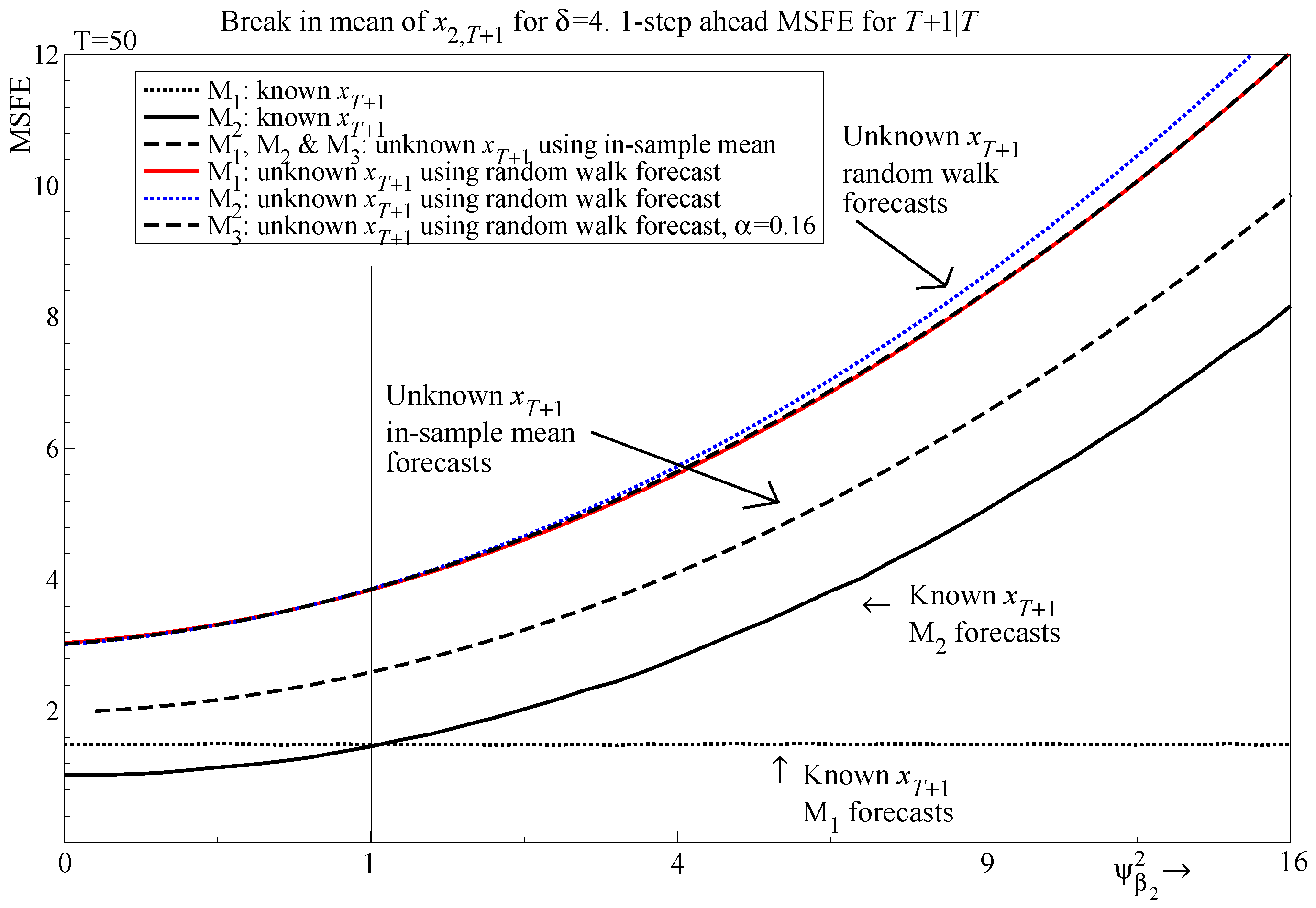
When ${\beta }_2=0$, both (23) and (28) collapse to ${\sigma }_{ϵ}^2+{\beta }_1^2$. The dampening of the squared location shift by ${\left(1-T^{-1}\right)}^2$ slightly improves the MSFE for the in-sample shift relative to an out-of-sample shift at larger ${\psi }_{\beta }^2$, as shown in Figure 7.

For a break out of sample, we find the analytic results for ${\mathrm{M}}_2$ are identical to those for ${\mathrm{M}}_1$ (see Section 5.4). For the in-sample break, the forecast error and MSFE for ${\mathrm{M}}_2$ does differ to that of ${\mathrm{M}}_1$ (see Appendix A.6 for analytic results). This is because the in-sample location shift affects $\rho$ which introduces a term similar to the squared location shift scaled by T in (28). Therefore, ${\mathrm{MSFE}}_1\ne {\mathrm{MSFE}}_2$ unless ${\beta }_2=0$, with ${\mathrm{M}}_2$ incurring a larger MSFE cost as ${\psi }_{\beta }^2$ increases due to misspecification, although the divergence is small even for small T, and disappears asymptotically.

6.3. Selecting Regressors

Selection follows from (12) and hence:

$${\mathrm{MSFE}}_3\approx {\mathrm{MSFE}}_1+\left(1-{\mathrm{p}}_{\alpha }\left({\psi }_{\beta }\right)\right)\left[{\sigma }_{ϵ}^2-{\beta }_1^2-{\rho }^2{\beta }_2^2+2T^{-1}\left({\sigma }_{\nu }^2+{\beta }_2^2{\delta }^2\right)\right].$$

The cost of omitting $x_2$ rises with ${\beta }_2^2{\delta }^2$, although increases in ${\beta }_2$ will raise ${\psi }_{\beta }^2$ and hence raise the probability of retaining $x_2$, albeit unconnected with the magnitude of ${\delta }^2$. As the location shift is scaled by T, ${\mathrm{MSFE}}_3\to {\mathrm{MSFE}}_1$ as $T\to \infty$.

6.4. Forecasting Regressors Using a Random Walk

From the previous analysis in Section 6.2, knowledge of the break at T brought little benefit when using in-sample means as forecasts. However, the random walk should do better when the break occurs at T as opposed to $T+1$. As before:

$${\tilde{\tilde{x}}}_{1,T+1|T}=x_{1,T}\mathrm{and}{\tilde{\tilde{x}}}_{2,T+1|T}=x_{2,T},$$

but now $\mathrm{E}\left[x_{1,T}\right]={\mu }_1$ and $\mathrm{E}\left[x_{2,T}\right]={\mu }_2+\delta$, and hence $\mathrm{E}\left[\Delta x_{1,T+1}\right]=0$ and $\mathrm{E}\left[\Delta x_{2,T+1}\right]=0$ as well.

Given the unbiased forecasts of the exogenous regressors, it follows that the forecasts for ${\mathrm{M}}_1$ are unbiased (see Appendix A.7) when the parameter estimates are unbiased. The MSFE for ${\mathrm{M}}_1$ is:

$${\mathrm{MSFE}}_1=\mathrm{E}\left[{\overline{\widehat{ϵ}}}_{T+1|T}^2\right]=2\left({\beta }_1^2+{\beta }_2^2\right)+4\rho {\beta }_1{\beta }_2+{\sigma }_{ϵ}^2\left(1+\frac{2}{T}+\frac{{\delta }^2}{T\left(1-{\rho }^2\right)}\right).$$

(29)

When ${\beta }_2=0$, the MSFE is similar to that of the out-of-sample break case, where the random walk is costly as forecasts of both $x_{1,T+1}$ and $x_{2,T+1}$ are inefficient. However, (29) does depend on the magnitude of the shift independently of ${\beta }_2$, unlike (26). ${\mathrm{MSFE}}_1$ is a function of ${\psi }_{\beta }^2$, increasing as ${\psi }_{\beta }^2$ increases, unlike in the known regressor case. But it does so more slowly than for breaks out of sample, or breaks in sample using the in-sample mean. As ${\psi }_{\beta }^2$ increases, the break at T in ${\mu }_2$ has a larger effect on the dependent variable, and hence the benefits of using a random walk forecast of $x_{2,T+1}$ are larger.

${\mathrm{M}}_2$ will suffer when ${\beta }_2\ne 0$ as the forecasts will be biased. The MSFE for ${\mathrm{M}}_2$ is:

$${\mathrm{MSFE}}_2=\mathrm{E}\left[{\widetilde{\overline{ϵ}}}_{T+1|T}^2\right]={\beta }_2^2\left({\delta }^2+{\rho }^2+1\right)+2{\beta }_1^2+4\rho {\beta }_1{\beta }_2+{\sigma }_{ϵ}^2\left(1+T^{-1}+T^{-2}{\psi }_{\beta }^2\right),$$

(30)

so no robustness in the sense of reducing bias is achieved unless ${\beta }_2=0$. When ${\beta }_2=0$, ${\mathrm{MSFE}}_2<{\mathrm{MSFE}}_1$, but the bias from not including a random walk, and hence unbiased, forecast of $x_{2,T+1}$ quickly outweighs parameter estimation costs as ${\psi }_{\beta }^2$ increases.

Solving for ${\mathrm{MSFE}}_2<{\mathrm{MSFE}}_1$ results in:

$${\psi }_{\beta }^2<\frac{\left(1-{\rho }^2\right)+{\delta }^2}{\left(1-{\rho }^2\right)\left(T^{-1}-1\right)+{\delta }^2}.$$

(31)

The break term dominates and offsets on the numerator and denominator, leading to a trade-off at ≈1 with deviations scaled by $T^{-1}$. For $\rho =0.5$, $T=100$ and $\delta =4$, ${\mathrm{MSFE}}_2$ dominates when ${\psi }_{\beta }=1.05$. Interestingly, the cut-off is slightly above 1 for this case, compared to slightly below 1 for the known breaks out-of-sample case, but the results still imply that a selection significance level of approximately 16% would be optimal to trade-off the cost of estimating an additional parameter.

Figure 8 records the MSFEs from ${\mathrm{M}}_1$ (29), ${\mathrm{M}}_2$ (30) and three values of ${\mathrm{M}}_3$ (A4) for the analytic results. There is a clear trade-off at ${\psi }_{\beta }^2\approx 1$, just as in the known breaks case.

6.5. Selecting Forecasted Regressors

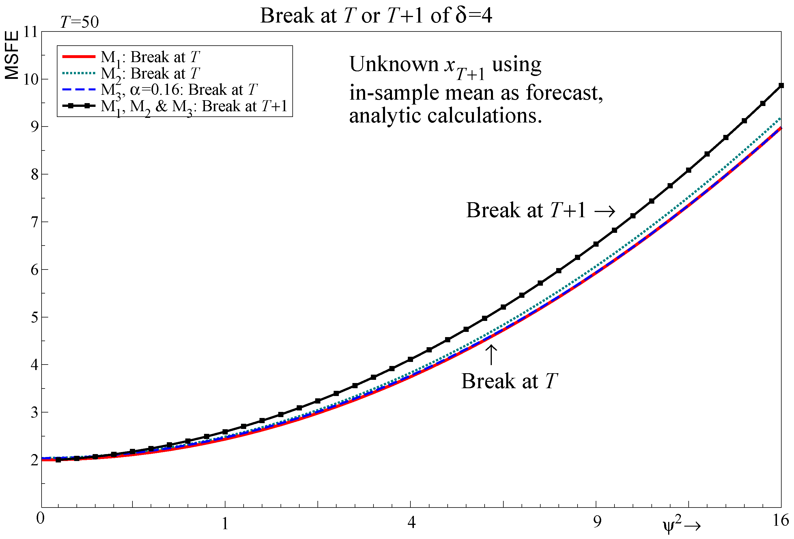
The final step is to compute the MSFE for ${\mathrm{M}}_3$ for the random walk forecast, reported in Appendix A.7. Just as regression models are usually selected, that will occur for any forecasting devices designed to minimize systematic bias. As with Figure 5, selection between ${\mathrm{M}}_1$ and ${\mathrm{M}}_2$ can be advantageous even for these forecasting devices as seen in Figure 8. Selection outperforms ${\mathrm{M}}_1$ for ${\psi }_{\beta }^2<1$, and remains close to the ${\mathrm{MSFE}}_1$ at $\alpha =0.05$ and $\alpha =0.16$, again in all cases matching or outperforming always using ${\mathrm{M}}_2$.

A comparison with the MSFE for the in-sample mean forecasts, also recorded in Figure 8, suggests a possible forecast improvement. If the regressor that breaks at T is known, combining the in-sample mean forecast for ${\mathrm{M}}_1$ with the random walk forecast for ${\mathrm{M}}_2$ will improve forecast performance (shifting the MSFE curves for the random walk forecast down by approximately 1). As the number of regressors increases, the forecasting method for each contemporaneous regressor will have a cumulative impact. However, as the break occurs in sample, methods to detect breaks at the forecast origin such as impulse indicator saturation (IIS) could be used to guide the forecaster to the most appropriate forecasting device.4 Selection between forecasting devices that minimize systematic bias versus those that trade-off bias and variance requires pre-testing and would only help for in-sample shifts; see, e.g., Chu et al. (1996).

Thus, selection can be valuable for forecasting to the extent that it retains relevant regressors that shift (here, $x_2$), and also if it eliminates irrelevant regressors that shift, as considered in Section 9.

6.6. Forecasting the Dependent Variable Using a Random Walk

If a break is suspected, an alternative to the approaches considered so far is to use a knowingly misspecified model of the conditional DGP. One possibility is to use a random walk forecast for y, with the advantage that $y_T$ is known and avoids the need to forecast $x_{1,T+1}$ and $x_{2,T+1}$. Hendry and Mizon (2012) derive a forecast-error taxonomy for open models that demonstrates the numerous additional forecast errors that arise from forecasting regressors offline in open models. They show that, in some cases, it can pay to use a misspecified model rather than to forecast the regressors offline. The forecast device is:

$${\tilde{\tilde{y}}}_{T+1|T}=y_T.$$

Then

$$y_T={\mu }_y+{\beta }_2\delta +{\beta }_1{\eta }_{1,T}+{\beta }_2{\eta }_{2,T}+{ϵ}_T$$

is a noisy one-observation estimator of $\left({\mu }_y+{\beta }_2\delta \right)$. The outturn at $T+1$ is:

$$y_{T+1}=\left({\mu }_y+{\beta }_2\delta \right)+{\beta }_1\Delta {\eta }_{1,T+1}+{\beta }_2\Delta {\eta }_{2,T+1}+{ϵ}_{T+1}+{\beta }_1{\eta }_{1,T}+{\beta }_2{\eta }_{2,T}.$$

The forecast error is given by:

$${\widetilde{\tilde{ϵ}}}_{T+1|T}=y_{T+1}-{\tilde{\tilde{y}}}_{T+1|T}={\beta }_1\Delta {\eta }_{1,T+1}+{\beta }_2\Delta {\eta }_{2,T+1}+\Delta {ϵ}_{T+1},$$

which is unbiased and has a MSFE of:

$${\mathrm{MSFE}}_4=\mathrm{E}\left[{\widetilde{\tilde{ϵ}}}_{T+1|T}^2\right]=2\left({\beta }_1^2+{\beta }_2^2\right)+4\rho {\beta }_1{\beta }_2+2{\sigma }_{ϵ}^2.$$

This is independent of $\delta$ so should perform relatively the best when ${\delta }^2$ is large, although performs worse than random walk forecasts for $x_{1,T+1}$ and $x_{2,T+1}$ when ${\psi }_{\beta }^2$ is small; see Figure 8. The forecasts are invariant to omitting $x_2$ since this random walk forecast is independent of the regressors, which is a major advantage and negates the role of selection. However, there is a cost when the model is correctly specified. The results in the simulation below suggest that such an approach should be viewed as complementary, with forecast pooling across selected conditional models and misspecified robust devices designed to mitigate bias frequently outperforming individual methods.

7. Summary of Analytic Results and the Impact of Selection

The theoretical analysis has established four results.

• Regressors should be retained if ${\psi }_{\beta }\ge 1$. This is established for DGPs that are stationary or with a break out of sample for known regressors and a break in sample for random walk forecasts.
• For the two-regressor case, ${\psi }_{\beta }=1$ maps to $\alpha \approx 0.16$. Selection delivers improvements to the one-step-ahead MSFE for ${\psi }_{\beta }<1$ and can be close to the correct model specification for ${\psi }_{\beta }>1$, with the largest deviations occurring at intermediate values of ${\psi }_{\beta }$.
• If there are breaks out of sample and contemporaneous regressors need to be forecast, the break dominates the MSFE and selection plays almost no role. Similar results are found even if the break occurs at the end of the sample, but the in-sample mean is used to forecast the regressors.
• Random walk forecasts are costly if there are no breaks (forecasting $x_{1,T+1}$) or if the breaks are unpredictable (a break at $T+1$ and forecasting $T+1|T$). However, they improve MSFE when the break is predictable (break at T and forecasting $T+1|T$).

Table 3. Ratio of MSFE to that of ${\mathrm{MSFE}}_1$, $T=50$. ${\mathrm{M}}_2$ has no selection ($\alpha =0$); selection in ${\mathrm{M}}_3$ at $\alpha$.

	MSFE Relative to ${\mathbf{MSFE}}_1$
	Model	${\mathit{\psi }}_{\mathit{\beta }}^2=0$	${\mathit{\psi }}_{\mathit{\beta }}^2=1$	${\mathit{\psi }}_{\mathit{\beta }}^2=4$	${\mathit{\psi }}_{\mathit{\beta }}^2=9$	${\mathit{\psi }}_{\mathit{\beta }}^2=16$
Section 4.1 and Section 4.2 No shift with known future regressors
	$\alpha =0\left({\mathrm{M}}_2\right)$	0.981	1.001	1.060	1.158	1.295
	$\alpha =0.001$	0.981	1.000	1.051	1.093	1.068
	$\alpha =0.05$	0.982	1.000	1.027	1.023	1.006
	$\alpha =0.16$	0.984	1.000	1.016	1.008	1.001
Section 5.2 and Section 5.3 Out-of-sample shift with known future regressors
	$\alpha =0\left({\mathrm{M}}_2\right)$	0.709	1.014	1.927	3.450	5.582
	$\alpha =0.001$	0.709	1.013	1.836	2.505	2.095
	$\alpha =0.05$	0.724	1.011	1.449	1.366	1.095
	$\alpha =0.16$	0.756	1.009	1.256	1.136	1.022
Section 5.4 Out-of-sample shift with mean forecast of future regressors
	$\alpha =0\left({\mathrm{M}}_2\right)$	1.000	1.000	1.000	1.000	1.000
	$\alpha =0.001$	1.000	1.000	1.000	1.000	1.000
	$\alpha =0.05$	1.000	1.000	1.000	1.000	1.000
	$\alpha =0.16$	1.000	1.000	1.000	1.000	1.000
Section 5.5 Out-of-sample shift with random walk forecast of future regressors
	$\alpha =0\left({\mathrm{M}}_2\right)$	0.993	1.004	1.020	1.034	1.043
	$\alpha =0.001$	0.993	1.004	1.018	1.021	1.010
	$\alpha =0.05$	0.994	1.003	1.010	1.005	1.001
	$\alpha =0.16$	0.994	1.002	1.006	1.002	1.000
Section 6.2 and Section 6.3 In-sample shift with mean forecast of future regressors
	$\alpha =0\left({\mathrm{M}}_2\right)$	1.020	1.021	1.022	1.023	1.024
	$\alpha =0.001$	1.020	1.021	1.020	1.014	1.006
	$\alpha =0.05$	1.019	1.017	1.011	1.004	1.000
	$\alpha =0.16$	1.017	1.014	1.006	1.001	1.000
Section 6.4 and Section 6.5 In-sample shift with random walk forecast of future regressors
	$\alpha =0\left({\mathrm{M}}_2\right)$	0.871	0.990	1.273	1.653	2.078
	$\alpha =0.001$	0.871	0.990	1.246	1.401	1.258
	$\alpha =0.05$	0.878	0.991	1.132	1.097	1.022
	$\alpha =0.16$	0.892	0.993	1.075	1.036	1.005

summarises the results for specific parameters using $T=50$ ($T=100$ is in

Table A1. Ratio of MSFE to that of ${\mathrm{MSFE}}_1$. $T=100$, otherwise as Table 3.

	MSFE Relative to ${\mathbf{MSFE}}_1$
Model	${\mathit{\psi }}_{\mathit{\beta }}^2=0$	${\mathit{\psi }}_{\mathit{\beta }}^2=1$	${\mathit{\psi }}_{\mathit{\beta }}^2=4$	${\mathit{\psi }}_{\mathit{\beta }}^2=9$	${\mathit{\psi }}_{\mathit{\beta }}^2=16$
Section 4.1 and Section 4.2 No shift with known future regressors
$\alpha =0\left({\mathrm{M}}_2\right)$	0.990	1.000	1.030	1.079	1.149
$\alpha =0.001$	0.990	1.000	1.026	1.048	1.035
$\alpha =0.05$	0.991	1.000	1.014	1.012	1.003
$\alpha =0.16$	0.992	1.000	1.008	1.004	1.001
Section 5.2 and Section 5.3 Out-of-sample shift with known future regressors
$\alpha =0\left({\mathrm{M}}_2\right)$	0.827	1.008	1.551	2.457	3.724
$\alpha =0.001$	0.827	1.008	1.497	1.895	1.651
$\alpha =0.05$	0.836	1.007	1.267	1.217	1.056
$\alpha =0.16$	0.855	1.005	1.152	1.081	1.013
Section 5.4 Out-of-sample shift with mean forecast of future regressors
$\alpha =0\left({\mathrm{M}}_2\right)$	1.000	1.000	1.000	1.000	1.000
$\alpha =0.001$	1.000	1.000	1.000	1.000	1.000
$\alpha =0.05$	1.000	1.000	1.000	1.000	1.000
$\alpha =0.16$	1.000	1.000	1.000	1.000	1.000
Section 5.5 Out-of-sample shift with random walk forecast of future regressors
$\alpha =0\left({\mathrm{M}}_2\right)$	0.997	1.002	1.013	1.024	1.033
$\alpha =0.001$	0.997	1.002	1.012	1.015	1.008
$\alpha =0.05$	0.997	1.002	1.006	1.004	1.001
$\alpha =0.16$	0.997	1.001	1.004	1.001	1.000
Section 6.2 and Section 6.3 In-sample shift with mean forecast of future regressors
$\alpha =0\left({\mathrm{M}}_2\right)$	1.010	1.009	1.008	1.007	1.007
$\alpha =0.001$	1.010	1.009	1.008	1.005	1.002
$\alpha =0.05$	1.010	1.008	1.004	1.001	1.000
$\alpha =0.16$	1.008	1.006	1.002	1.000	1.000
Section 6.4 and Section 6.5 In-sample shift with random walk forecast of future regressors
$\alpha =0\left({\mathrm{M}}_2\right)$	0.931	0.994	1.155	1.386	1.661
$\alpha =0.001$	0.931	0.994	1.140	1.237	1.158
$\alpha =0.05$	0.934	0.995	1.075	1.058	1.014
$\alpha =0.16$	0.942	0.996	1.043	1.021	1.003

in Appendix B). For each scenario, the ratio of ${\mathrm{MSFE}}_j$/${\mathrm{MSFE}}_1$ for $j=2,3$ is reported. ${\mathrm{MSFE}}_2$ has no selection, and is therefore listed as $\alpha =0$, while three values of $\alpha$ are used for ${\mathrm{MSFE}}_3$. The squared noncentralities ${\psi }_{\beta }^2=0,1,4,9,16$ capture the full hump shape seen in the figures above.

${\mathrm{M}}_2$ is the correct model in the column labelled ${\psi }_{\beta }^2=0$, so the ratio of ${\mathrm{MSFE}}_2/{\mathrm{MSFE}}_1$ measures the cost of over-specification. The gains can be substantial in some cases, almost 30% for a break out of sample with known regressors, but in other cases including $x_{2,t}$ is not at all costly despite its irrelevance. Tighter selection for ${\mathrm{M}}_3$ is close to ${\mathrm{M}}_2$ as $x_{2,t}$ will be omitted more frequently, but even at $\alpha =0.16$ the ratio for ${\mathrm{M}}_3$ is close to the ratio for ${\mathrm{M}}_2$, suggesting that selection is not costly.

Moving to the next column highlights the ${\psi }_{\beta }=1$ trade-off, with all cases almost exactly equal to one. A cut-off slightly lower than one was found in (19), which is reflected in the ratio marginally greater than one. Conversely, (31) found a cut-off slightly larger than one, resulting in a ratio slightly below one, but the differences are small.

Next, consider the columns labelled ${\psi }_{\beta }^2=4,9$, and 16. ${\mathrm{M}}_1$ is the correct model so the objective is to minimize the ratio. In some cases ${\mathrm{M}}_2$ performs poorly, but ${\mathrm{M}}_3$ at $\alpha =0.16$ is frequently very close to 1, i.e., ${\mathrm{MSFE}}_1$. Selection forecast performance tends to be worse at ${\psi }_{\beta }^2=4$, but as the signal for $x_2$ increases, the probability of retaining $x_2$ increases so the selected model is closer to ${\mathrm{M}}_1$. The benefits of selection vary by case. For example, for a break at T using in-sample means, selection at $\alpha =0.16$ delivers a 2.4% improvement relative to ${\mathrm{M}}_2$ for ${\psi }_{\beta }=4$, compared to a halving of the ratio for the random walk. In almost every setting, ${\mathrm{MSFE}}_3$ is close to ${\mathrm{MSFE}}_1$ so the costs of selection are usually small, irrespective of the noncentrality. In that sense, model selection acts to reduce the risk relative to the worst model. Conversely, the costs of unmodeled shifts are very large, up to almost 8-fold greater than the baseline stationary ${\mathrm{MSFE}}_1$.

These results show that even facing breaks, the well-known trade-off for selecting variables in forecasting models, namely that variables should be retained if their noncentralities exceed 1, still applies, resulting in much looser significance levels than typically used. The problem with such an approach is that when many ${\beta }_{2,i}=0$ but are subject to location shifts, ${\mathrm{M}}_1$, which erroneously includes $x_{2,t}$ in the model, will perform worse. Loose significance levels increase the chance that irrelevant variables with ${\psi }_{\beta }=0$ are retained by being adventitiously significant for that draw. To evaluate this effect, the next section undertakes a simulation study of selection in models with ten irrelevant and five relevant exogenous regressor variables confronting a variety of shifts.

8. Simulation Design

We generalize the above analysis using Monte Carlo analysis, formalizing the DGP and models that are estimated. We consider larger models with dynamics, evaluating for a range of strategies to forecast future values of the regressors, different significance levels, and different configurations of out-of-sample breaks. The next section then evaluates the simulation results.

8.1. Data Generation Process

The DGP is for a scalar dependent variable $y_t$, and N regressors ${\mathbf{x}}_t={(x_{1,t},\dots ,x_{N,t})}^{\prime }$. There are n regressors that are relevant, i.e., have a nonzero coefficient in the DGP for $y_t$, and $N-n$ that are irrelevant with coefficient zero.

We wish to introduce breaks either in relevant, or irrelevant, or both types of regressors. For convenience we assume that the regressors are ordered by increasing significance (i.e., squared noncentrality ${\psi }_{{\beta }_i}^2$). The DGP for y is an AR(1) with regressors:

$$y_t^{*}={\beta }_0+{\beta }_y{y}_{t-1}^{*}+\sum _{j=1}^N{\beta }_j{x}_{j,t}+{ϵ}_t,{ϵ}_t\sim \mathrm{IN}[0,{\sigma }_{ϵ}^2],t=-Q+1,\dots ,0,1,\dots ,T+H.$$

(32)

The regressors are independent of each other and (in sample) have a common autoregressive coefficient $\lambda$ and mean $\delta /\left(1-\lambda \right)$. We allow for a break in observations $T+1$ and $T+2$, using subscript I if the break applies to xs that are irrelevant in (32) (i.e., have a coefficient of zero) and R for those that are relevant:

$$\begin{array}{ccc}\hfill x_{j,t}& =\delta +\lambda x_{j,t-1}+{\eta }_{j,t},{\eta }_{j,t}\sim \mathrm{IN}[0,1],\hfill & \hfill j=1,\dots ,N,t=-Q+1,\dots ,T,T+3,\dots ,\\ \hfill x_{j,t}& ={\delta }_I+{\lambda }_I{x}_{j,t-1}+{\eta }_{j,t},{\eta }_{j,t}\sim \mathrm{IN}[0,1],\hfill & \hfill j=1,\dots ,N-n,t=T+1,T+2,\\ \hfill x_{j,t}& ={\delta }_R+{\lambda }_R{x}_{j,t-1}+{\eta }_{j,t},{\eta }_{j,t}\sim \mathrm{IN}[0,1],\hfill & \hfill j=N-n+1,\dots ,t=T+1,T+2.\end{array}$$

(33)

Throughout, we set ${\sigma }_{ϵ}^2=1$, ${\beta }_0=5$, ${\beta }_y=0.5$, $\delta =2$, $N=15$. Fifty initial observations are discarded ($Q=50$). We set observation zero equal to twenty in each replication, giving the generated data as:

$$y_t=y_t^{*}+20-y_0^{*}.$$

(34)

The remaining coefficients in (32) are specified through their noncentralities. We run three alternative experiments:

$$\begin{array}{cc}\mathit{\psi }\left(1\right):\hfill & {\mathit{\psi }}_{\beta }={\left(0,0,0,0,0,1.2,1.2,1.2,1.2,1.2,1.2,1.2,1.2,1.2,1.2\right)}^{\prime },\hfill \\ \mathit{\psi }\left(2\right):\hfill & {\mathit{\psi }}_{\beta }={\left(0,0,0,0,0,0,0,0.5,1,1.5,2,3,4\right)}^{\prime },\hfill \\ \mathit{\psi }\left(4\right):\hfill & {\mathit{\psi }}_{\beta }={\left(0,0,0,0,0,0,0,0,0,0,0,0,4,4,4\right)}^{\prime }.\hfill \end{array}$$

(35)

Then ${\beta }_j={\psi }_{{\beta }_j}{\left\{(T-N-2)\mathrm{V}\left[x_{j,t}\right]\right\}}^{-1/2}$, using the in-sample variances computed over $t=1,\dots ,T$. This ensures that the t-values in the estimates of (32) will be equal to ${\psi }_{{\beta }_j}$ on average. Note that the noncentralities in each specification sum to twelve, and have $n=10,6,3$ respectively.

With common coefficients $\delta$ and $\lambda$, the regressors are exchangeable in analytical calculations. The unconditional process of each $x_j$, in the absence of any break, has mean $\overline{x}=\delta /(1-\lambda )$ and variance ${(1-{\lambda }^2)}^{-1}$. When $\delta =2$ and $\lambda =0.75$, the steady state for $y_t^{*}$ is then $\overline{y}=10+2\times 8\times 12\times {\{83/(1-{0.775}^2)\}}^{-1/2}\approx 10+16\times 0.87=23.9$, using total noncentrality of 12, $\overline{x}=8$, $T=100$, $N=15$. The degrees-of-freedom adjustment counts N, the intercept, and the lagged dependent variable.

Breaks in the process for the target variable y are introduced through breaks in the regressors. During the break, ${\delta }_R=-0.3\equiv {\delta }_{\Delta }$, so $\delta$ drops by $-2.3$. Keeping $\lambda$ unchanged, the equilibrium changes from $\overline{x}=8$ to ${\overline{x}}_{\Delta }=-1.2$, which is a shock of six unconditional standard errors. The impact on $y_t$ depends on the coefficients ${\beta }_j$. To quantify this, it is convenient to assume that the processes are at their unconditional means, after which we follow the shocks through the dynamic system, ignoring the disturbances. The impact on x when the coefficients change from $(\delta ,\lambda )=(2,0.75)$ to $({\delta }_{\Delta },{\lambda }_{\Delta })$ is given in

Table 4. Impact on x when coefficients change from $(\delta ,\lambda )=(2,0.75)$ to $({\delta }_{\Delta },{\lambda }_{\Delta })$.

$({\mathit{\delta }}_{\mathsf{\Delta }},{\mathit{\lambda }}_{\mathsf{\Delta }})=$	(2, 0.75)	(−0.3, 0.75)	(−0.3, 0.95)	(−0.3, 0.05)	(2, 0.05)	(2, 0.95)
$x_{j,T+1|T}$	8	5.7	7.3	0.1	2.4	9.6
$x_{j,T+2|T+1}$	8	4.0	6.6	−0.3	2.1	11.1
$x_{j,T+3|T+2}$	8	5.0	7.0	1.8	3.6	10.3

.

The process reverts to the original coefficients at $T+3$, aiming to capture qualitatively aspects of a sustained but temporary structural break, such as the Great Financial Crisis or the COVID-19 pandemic. The impact of the break on $y_{j,T+1|T}$ is $0.87$ times the new x. For $(-0.3,0.95)$ this is a change of $0.6$, well below y’s conditional standard error of unity.

Table 5. Configurations of breaks in the simulations.

	${\mathit{\delta }}_{\mathsf{\Delta }}$	${\mathit{\lambda }}_{\mathsf{\Delta }}$
No break	2	0.75
Break in mean	−0.3	0.75
Break in slope (a)	2	0.95
Break in slope (b)	2	0.05
Break in mean and slope (a)	−0.3	0.95
Break in mean and slope (b)	−0.3	0.05

lists the break settings we consider. The upward break in slope (a) pushes the process towards a unit root, while the downward break in slope (b) makes it almost white noise. Figure 9 plots the second half of $y_t$ for one replication of the DGP and for each of the five specifications of the break. This is for $T=100$ and after discarding the initial observations. The break lasts for two observations in the forecast period, after which the DGP reverts to the settings without break. Figure 9 illustrates the low impact of the break in mean and slope when $({\delta }_{\Delta },{\lambda }_{\Delta })=(-0.3,0.95)$.

The design (33) allows for breaks in relevant variables, in irrelevant variables, or in both. In the last case: ${\delta }_R={\delta }_I={\delta }_{\Delta }$ and ${\lambda }_R={\lambda }_I={\lambda }_{\Delta }$. Breaks in irrelevant variables do not affect y, but can have an impact on forecasts if the irrelevant variables are used in the forecasts’ construction. However, when forecasting for $T+1|T$, such breaks have no impact at all, because the future $x_{T+1}$s are not yet known.

8.2. Models and Forecast Devices

We generate $Q+T+H$ observations from DGP (32)–(34), discarding the initial Q. The starting point for modeling is the general unrestricted model (GUM):

$$y_t={\beta }_0+{\beta }_y{y}_{t-1}+\sum _{j=1}^N{\beta }_j^{*}{x}_{j,t}+\sum _{j=1}^N{\gamma }_j^{*}{x}_{j,t-1}+{ϵ}_t,\mathrm{for}t=1,\dots ,T.$$

(36)

An asterisk indicates that model selection is used, so the intercept and lagged y are not selected over but are always retained. Model selection is only performed once for each replication, but the selected model is re-estimated by ordinary least squares (OLS) each time that we forecast given data up to $T+h-1$:

$$y_t={\beta }_0+{\beta }_y{y}_{t-1}+\sum _{{\widehat{\beta }}_j^{*}\ne 0}{\beta }_j{x}_{j,t}+\sum _{{\widehat{\gamma }}_j^{*}\ne 0}{\gamma }_j{x}_{j,t-1}+{\epsilon }_t,\mathrm{for}t=h,\dots ,T+h-1.$$

(37)

Only one-step-ahead forecasts are generated and evaluated:

$${\widehat{y}}_{T+h|T+h-1}={\widehat{\beta }}_0+{\widehat{\beta }}_y{y}_{T+h-1}+\sum _{{\widehat{\beta }}_j^{*}\ne 0}{\widehat{\beta }}_j{\tilde{x}}_{j,T+h}+\sum _{{\widehat{\gamma }}_j^{*}\ne 0}{\widehat{\gamma }}_j{x}_{j,T+h-1}\mathrm{for}h=1,\dots ,H.$$

(38)

The out-of-sample values ${\tilde{x}}_{j,T+h}$ of the regressors in (38) are unknown when forming the forecasts. We consider a range of forecast devices that can supply these missing values:

inf: 

future outcomes: ${\tilde{x}}_{j,T+h}=x_{j,T+h}$;

avg: 

the in-sample average: ${\tilde{x}}_{j,T+h}={\sum }_{t=h}^{T+h-1}{x}_{j,t}/T$;

arx: 

an AR(1) for each regressor: ${\tilde{x}}_{j,T+h}={\widehat{\mu }}_j+{\widehat{\rho }}_j{x}_{j,T+h-1}$, estimated by OLS for each horizon from:

$$x_{j,t}={\mu }_j+{\rho }_j{x}_{j,t-1}+u_{j,t},t=h,\dots ,T+h-1;$$

(39)

rwx: 

the random walk forecast: ${\tilde{x}}_{j,T+h}=x_{j,T+h-1}$;

rdx: 

a random walk with differencing (Hendry 2006), using differenced estimates from (39):

$${\tilde{x}}_{j,T+h}=x_{j,T+h-1}+{\widehat{\rho }}_j\Delta x_{j,T+h-1}.$$

cax: 

Cardt forecast of ${\tilde{x}}_{j,T+h}$.

In addition, several alternatives that ignore the regressors are considered:

rwy: 

a random walk forecast: ${\widehat{y}}_{T+h}=y_{T+h-1}$;

ary: 

an AR(1) forecast: ${\widehat{y}}_{T+h}={\widehat{\gamma }}_0+{\widehat{\gamma }}_1{y}_{T+h-1}$, estimated by OLS for each horizon;

cay: 

Cardt forecasts of ${\widehat{y}}_{T+h}$.

Model selection is performed using Autometrics (Doornik 2009) for a range of target significance levels $\alpha =\left(0.001,0.01,0.05,0.1,0.16,0.32\right)$. Forecasting from a re-estimated GUM (37) without selection is also considered (i.e., $\alpha =1$). Dropping all regressors (i.e., $\alpha =0$) leaves the AR(1) model for $y_t$.

The devices that forecast the regressors supply plug-in values to allow forecasting with the GUM (36), as well as the reductions (37) of the GUM, at a range of nominal significance levels. Device inf uses future outcomes, making it infeasible for stochastic variables. Note that all devices using regressors benefit from some knowledge that is not available in practice, namely that the DGP is nested in the GUM, and the GUM is not misspecified. The fact that the regressors are exchangeable and break at the same time in the same way may also help: finding just one that matters could already improve the forecasts.

Cardt is a slightly improved version of Card (calibrated average of rho and delta methods), see Doornik et al. (2020a), which performed very well in the M4 forecast competition of Makridakis et al. (2020). Cardt averages forecasts from a differenced, autoregressive, and a moving average model. These are then treated as future observations in a calibration model with richer autoregressive structure. The full procedure is documented in Castle et al. (2021). Cardt pays particular attention to seasonality, which is irrelevant here. We use Cardt to make four forecasts, then use the first of these. The method will take logarithms by default. Switching that off makes little difference in these experiments. Cardt is used in daily COVID-19 forecasts of Doornik et al. (2020b).

8.3. Selecting Regressors

The noncentrality ${\mathit{\psi }}_{\beta }$ in the DGP affects the probabilities of retaining a variable in the model selection procedure.

Table 6. Probability of retaining one or all variables when the coefficients have the specified noncentrality, assuming independence at nominal significance $\alpha$ and Student-t(83) distribution.

	${\mathit{\psi }}_{\mathit{\beta }}=1.2$		${\mathit{\psi }}_{\mathit{\beta }}=0.5$	${\mathit{\psi }}_{\mathit{\beta }}=1$	${\mathit{\psi }}_{\mathit{\beta }}=1.5$	${\mathit{\psi }}_{\mathit{\beta }}=2$	${\mathit{\psi }}_{\mathit{\beta }}=3$	${\mathit{\psi }}_{\mathit{\beta }}=4$	Joint	Average	${\mathit{\psi }}_{\mathit{\beta }}=4$
$\mathit{\alpha }$	$\mathit{n}\mathbf{=}\mathbf{1}$	$\mathit{n}\mathbf{=}\mathbf{10}$	$\mathit{n}\mathbf{=}\mathbf{1}$	$\mathit{n}\mathbf{=}\mathbf{1}$	$\mathit{n}\mathbf{=}\mathbf{1}$	$\mathit{n}\mathbf{=}\mathbf{1}$	$\mathit{n}\mathbf{=}\mathbf{1}$	$\mathit{n}\mathbf{=}\mathbf{1}$	$\mathit{n}\mathbf{=}\mathbf{6}$	$\mathit{n}\mathbf{=}\mathbf{6}$	$\mathit{n}\mathbf{=}\mathbf{1}$	$\mathit{n}\mathbf{=}\mathbf{3}$
0.001	0.015	0.000	0.002	0.009	0.030	0.081	0.341	0.721	0.000	0.197	0.721	0.375
0.01	0.077	0.000	0.018	0.053	0.130	0.263	0.641	0.912	0.000	0.336	0.912	0.758
0.05	0.216	0.000	0.070	0.163	0.313	0.504	0.843	0.976	0.001	0.478	0.976	0.930
0.1	0.322	0.000	0.124	0.254	0.435	0.631	0.907	0.989	0.008	0.557	0.989	0.968
0.16	0.414	0.000	0.181	0.339	0.533	0.719	0.941	0.994	0.022	0.618	0.994	0.983
0.32	0.579	0.004	0.309	0.500	0.691	0.840	0.976	0.998	0.087	0.719	0.998	0.995

shows the probability of retaining one or all relevant regressors assuming independent t-tests. While the probability of retaining one variable may be quite large, the joint probability of retaining all can be extremely low. Thus, even using a significance level of 16%, many relevant variables will be omitted if their noncentralities are small. However, their contribution to explaining the dependent variable is also small and breaks in such variables will have a smaller effect.

The fraction of relevant variables that is retained in the Monte Carlo experiment is denoted the potency, and the fraction of irrelevant variables that is retained is denoted the gauge. We always retain the intercept and lagged y, so the GUM (36) has $2N$ possible variables to select over, of which n are relevant. For $m=1,\dots ,M$ replications we define the indicator function $\mathbf{1}\{·\}$ and:

$$\begin{array}{cc}\hfill {\mathrm{gauge}}_m=& \frac{1}{2N-n}\left[\sum _{j=1}^{N-n}\mathbf{1}\{{\widehat{\beta }}_{j,m}\ne 0\}+\sum _{j=1}^N\mathbf{1}\{{\widehat{\gamma }}_{j,m}\ne 0\}\right],\hfill \\ \hfill {\mathrm{potency}}_m=& \frac{1}{n}\sum _{j=N-n+1}^N\mathbf{1}\{{\widehat{\beta }}_{j,m}\ne 0\}.\hfill \end{array}$$

This is then averaged over all replications.

Table 7. Gauge and potency for three noncentrality designs, M = 10,000 replications.

	Gauge			Potency
$\mathit{\alpha }$	$\mathit{\psi }\mathbf{\left(}\mathbf{1}\mathbf{\right)}$	$\mathit{\psi }\mathbf{\left(}\mathbf{2}\mathbf{\right)}$	$\mathit{\psi }\mathbf{\left(}\mathbf{4}\mathbf{\right)}$	$\mathit{\psi }\mathbf{\left(}\mathbf{1}\mathbf{\right)}$	$\mathit{\psi }\mathbf{\left(}\mathbf{2}\mathbf{\right)}$	$\mathit{\psi }\mathbf{\left(}\mathbf{4}\mathbf{\right)}$
0.001	0.005	0.006	0.006	0.034	0.205	0.712
0.01	0.025	0.024	0.020	0.113	0.345	0.884
0.05	0.079	0.075	0.069	0.231	0.458	0.919
0.1	0.126	0.124	0.121	0.297	0.507	0.919
0.16	0.181	0.180	0.178	0.355	0.545	0.923
0.32	0.328	0.328	0.327	0.479	0.634	0.941

shows that the empirical gauge matches the theoretical probabilities in Table 6 when using Autometrics for selection: the gauge is higher than $\alpha$ but not by much. Potencies are close to the powers of one-off t-tests with the same noncentralities, up to $\alpha =0.1$, beyond that they fall behind. Consequently, it is appropriate to use Autometrics to investigate the theoretical results by simulating a more general setting, without concern that the selection algorithm will influence the results relative to the single t-test approach analyzed above.

9. Simulation Evidence

Simulation evidence is presented using the design of Section 8.1 and forecast devices of Section 8.2. All experiments use M = 10,000 and are implemented in Ox 9 (Doornik 2018) and PcGive (Hendry and Doornik 2018). We start with out-of-sample forecasts in Section 9.1, when the break is unanticipated. Then Section 9.2 compares breaks in relevant and irrelevant variables, Section 9.3 looks at forecasts after the break, Section 9.4 considers selection, Section 9.5 introduces pooled forecasts, and Section 9.6 summarizes.

9.1. Forecasting before the Break

The top half of

Table 8. No break and out-of-sample break. Ratio of MSFE to MSFE_ary forecasting $T+1|T$.

	$\mathit{\psi }\left(1\right)$				$\mathit{\psi }\left(2\right)$				$\mathit{\psi }\left(4\right)$
	inf	avg	arx	rwx	inf	avg	arx	rwx	inf	avg	arx	rwx
Ratio	No break
$\alpha =0$	1.00	1.00	1.00	1.00	1.00	1.00	1.00	1.00	1.00	1.00	1.00	1.00
$\alpha =0.001$	1.03	1.01	1.02	1.03	0.95	1.06	0.99	1.02	0.83	1.13	0.94	0.99
$\alpha =0.01$	1.08	1.06	1.05	1.08	0.93	1.11	0.98	1.02	0.79	1.17	0.93	0.97
$\alpha =0.05$	1.13	1.13	1.08	1.12	0.95	1.19	0.99	1.03	0.83	1.23	0.95	0.99
$\alpha =0.1$	1.16	1.18	1.09	1.13	0.99	1.23	1.01	1.06	0.87	1.27	0.97	1.02
$\alpha =0.16$	1.19	1.23	1.11	1.15	1.01	1.28	1.04	1.08	0.91	1.31	1.00	1.04
$\alpha =0.32$	1.25	1.36	1.15	1.19	1.09	1.38	1.09	1.13	0.99	1.41	1.05	1.09
GUM	1.34	1.51	1.20	1.23	1.18	1.50	1.13	1.17	1.08	1.52	1.10	1.14
MSFEary	1.15				1.31				1.43
Ratio	Average over five break types in relevant regressors
$\alpha =0$	1.00	1.00	1.00	1.00	1.00	1.00	1.00	1.00	1.00	1.00	1.00	1.00
$\alpha =0.001$	0.90	1.00	1.00	1.01	0.58	1.02	0.99	1.00	0.37	1.05	0.97	0.98
$\alpha =0.01$	0.74	1.01	1.01	1.02	0.42	1.04	0.99	0.99	0.28	1.06	0.97	0.97
$\alpha =0.05$	0.57	1.03	1.01	1.02	0.37	1.06	0.99	0.99	0.28	1.08	0.97	0.98
$\alpha =0.1$	0.52	1.05	1.02	1.03	0.37	1.07	0.99	1.00	0.29	1.09	0.98	0.98
$\alpha =0.16$	0.50	1.06	1.02	1.03	0.37	1.08	1.00	1.01	0.30	1.10	0.99	0.99
$\alpha =0.32$	0.48	1.10	1.03	1.04	0.38	1.11	1.01	1.02	0.32	1.13	1.00	1.01
GUM	0.49	1.13	1.05	1.05	0.41	1.14	1.03	1.03	0.35	1.16	1.01	1.02
MSFEary	18.58				18.80				18.98

is for the case without breaks, when forecasting $T+1|T$ is similar to forecasting $T+2|T+1$, etc. The table reports the ratio of the MSFE for devices inf, avg, arx, rwx respectively to the MSFE of ary for a range of significance levels $\alpha$. Selection at $\alpha =0$ implies dropping all the regressors, leaving an AR(1) in y, denoted ary. The bottom row of each half gives the MSFE of ary. Not selecting at all ($\alpha =1$) coincides with the GUM.

Without a break, knowing the future value of regressors, device inf, is only useful when they are significant. Using the sample mean avg never improves one-step forecasting relative to ary. This also holds when there is a break, and is even more pronounced for $T+2|T+1$ and $T+3|T+2$ (not shown). We see that ${\mathrm{MSFE}}_{ary}$ increases when there are more highly significant variables. There is an improvement over ary from forecasting the regressors with arx at strict significance levels for $\psi \left(4\right)$. In this stationary DGP without breaks, arx dominates rwx: it is better to model the regressors by an autoregression (the true model) than taking the last known value.

The bottom half of Table 8 is for the cases with an out-of-sample break in the relevant variables only. The ratios for the five break settings (in mean, in slope, and in mean and slope, for (a) and (b)) are averaged. Now it really would help to know the future. There is only a small penalty for including irrelevant regressors, as their influence is swamped by the break. Except for the sample means, both feasible methods perform on a par with ary. The infeasible device is best with loose selection, as was found theoretically.

9.2. Selection and Location of the Break

The design of the experiments allows for three locations of the break.

Table 9. Break in mean and slope (b). MSFE for different locations of the break.

			$\mathit{T}+1|\mathit{T}$				$\mathit{T}+2|\mathit{T}+1$				$\mathit{T}+3|\mathit{T}+2$
	$\mathit{\psi }$	Where	inf	avg	arx	rwx	inf	avg	arx	rwx	inf	avg	arx	rwx
$\alpha =0$ary	$\mathit{\psi }\left(1\right)$	Relevant	54.42				50.41				6.75
$\alpha =0.1$	$\mathit{\psi }\left(1\right)$	Relevant	16.44	54.49	54.50	54.60	10.67	60.24	18.33	11.24	3.51	33.30	3.03	3.48
GUM	$\mathit{\psi }\left(1\right)$	Relevant	11.43	54.78	54.63	54.77	10.15	60.60	13.56	9.76	2.89	41.42	2.43	4.15
$\alpha =0$ary	$\mathit{\psi }\left(1\right)$	All	54.42				50.41				6.75
$\alpha =0.1$	$\mathit{\psi }\left(1\right)$	All	18.32	54.49	54.50	54.60	11.19	61.32	18.71	11.70	3.32	33.28	2.89	3.61
GUM	$\mathit{\psi }\left(1\right)$	All	16.42	54.78	54.63	54.77	14.12	64.35	17.41	13.64	3.05	42.12	2.55	4.21
$\alpha =0$ary	$\mathit{\psi }\left(1\right)$	Irrel.	1.15				1.19				1.18
$\alpha =0.1$	$\mathit{\psi }\left(1\right)$	Irrel.	3.19	1.36	1.26	1.31	2.86	2.59	2.55	2.80	1.82	2.04	1.80	1.89
GUM	$\mathit{\psi }\left(1\right)$	Irrel.	6.71	1.75	1.39	1.42	5.74	6.16	5.38	5.52	2.18	3.39	2.02	2.00
$\alpha =0$ary	$\mathit{\psi }\left(2\right)$	Relevant	54.71				43.20				6.02
$\alpha =0.1$	$\mathit{\psi }\left(2\right)$	Relevant	7.90	54.86	54.82	54.98	4.84	61.25	12.40	5.43	2.64	37.40	2.51	3.87
GUM	$\mathit{\psi }\left(2\right)$	Relevant	7.60	55.05	54.94	55.17	6.73	58.20	10.67	6.58	2.68	40.60	2.47	4.31
$\alpha =0$ary	$\mathit{\psi }\left(2\right)$	All	54.71				43.20				6.02
$\alpha =0.1$	$\mathit{\psi }\left(2\right)$	All	11.05	54.86	54.82	54.98	6.76	62.80	13.90	7.23	2.65	37.15	2.59	4.27
GUM	$\mathit{\psi }\left(2\right)$	All	16.45	55.05	54.94	55.17	13.99	64.88	17.65	13.72	3.02	42.09	2.71	4.41
$\alpha =0$ary	$\mathit{\psi }\left(2\right)$	Irrel.	1.31				1.39				1.35
$\alpha =0.1$	$\mathit{\psi }\left(2\right)$	Irrel.	4.44	1.61	1.33	1.38	3.71	3.70	3.43	3.72	1.93	2.66	2.04	2.14
GUM	$\mathit{\psi }\left(2\right)$	Irrel.	10.46	1.97	1.48	1.53	8.90	9.47	8.59	8.78	2.36	4.11	2.28	2.26
$\alpha =0$ary	$\mathit{\psi }\left(4\right)$	Relevant	54.98				39.74				5.66
$\alpha =0.1$	$\mathit{\psi }\left(4\right)$	Relevant	4.38	54.98	55.03	55.31	2.64	61.84	9.54	3.19	2.00	38.64	2.21	4.54
GUM	$\mathit{\psi }\left(4\right)$	Relevant	4.56	55.27	55.21	55.51	4.20	56.23	8.50	4.27	2.42	39.53	2.45	4.47
$\alpha =0$ary	$\mathit{\psi }\left(4\right)$	All	54.98				39.74				5.66
$\alpha =0.1$	$\mathit{\psi }\left(4\right)$	All	8.45	54.98	55.03	55.31	5.27	63.59	11.82	5.71	2.31	38.55	2.55	5.00
GUM	$\mathit{\psi }\left(4\right)$	All	16.47	55.27	55.21	55.51	13.89	65.37	17.89	13.79	3.00	42.11	2.85	4.59
$\alpha =0$ary	$\mathit{\psi }\left(4\right)$	Irrel.	1.43				1.52				1.49
$\alpha =0.1$	$\mathit{\psi }\left(4\right)$	Irrel.	5.20	1.82	1.39	1.45	4.09	4.37	3.92	4.23	1.92	3.09	2.16	2.25
GUM	$\mathit{\psi }\left(4\right)$	Irrel.	13.46	2.17	1.57	1.63	11.33	12.03	11.05	11.29	2.47	4.62	2.44	2.43

gives the mean square forecast errors for a break in mean and slope (b), listing three cases.

Break in relevant regressors 

(${\delta }_R=-0.3,{\lambda }_R=0.05,{\delta }_I=\delta ,{\lambda }_I=\lambda$)

The break shows up in y through the relevant variables. Inclusion of irrelevant variables in the forecasting model is not costly relative to the impact of the break. Loose selection is preferred, because it includes more relevant variables. For $T+1|T$ selection has no impact because the break is not observed (except for known regressors). Including regressors in arx and rwx gives a substantial improvement over ary.

Break in irrelevant regressors 

(${\delta }_I=-0.3,{\lambda }_I=0.05,{\delta }_R=\delta ,{\lambda }_R=\lambda$)

There is no break in y, so any inclusion of irrelevant variables is costly, as their break offsets the small estimated coefficients. The more irrelevant variables included, the stronger this effect. The autoregression in y is almost always preferred.

Break in all regressors 

(${\delta }_R={\delta }_I=-0.3,{\lambda }_R={\lambda }_I=0.05$)

The y variable is identical to that of a break in relevant variables only. Selection is now a trade-off between including variables that matter and help with forecasting, and irrelevant variables that make forecasts worse. Including regressors in arx and rwx gives a substantial improvement over ary.

9.3. Forecasting after theBreak

We now dispense of inf for its infeasibility, and avg because it has the highest MSFE in all experiments.

Table 10. Ratio of MSFE to that of MSFE_ary. Selection at $\alpha =0.1$ for arx, rwx, rdx, and cax.

	$\mathit{T}+2|\mathit{T}+1$						$\mathit{T}+3|\mathit{T}+2$						$\mathit{T}+4|\mathit{T}+3$
	arx	rwx	rdx	cax	rwy	cay	arx	rwx	rdx	cax	rwy	cay	arx	rwx	rdx	cax	rwy	cay
	No break
$\mathit{\psi }\left(1\right)$	1.10	1.15	1.31	1.15	1.21	1.29	1.11	1.16	1.31	1.16	1.21	1.29	1.10	1.14	1.30	1.15	1.21	1.28
$\mathit{\psi }\left(2\right)$	1.00	1.04	1.24	1.05	1.14	1.19	1.02	1.07	1.29	1.08	1.15	1.22	1.01	1.06	1.25	1.06	1.15	1.21
$\mathit{\psi }\left(4\right)$	0.96	1.00	1.23	1.01	1.12	1.16	0.97	1.02	1.26	1.03	1.12	1.17	0.96	1.00	1.23	1.00	1.12	1.17
	Break in mean and slope (b) of irrelevant regressors
$\mathit{\psi }\left(1\right)$	2.14	2.35	3.30	2.33	1.21	1.29	1.53	1.61	1.75	1.64	1.21	1.29	1.20	1.25	1.35	1.25	1.21	1.28
$\mathit{\psi }\left(2\right)$	2.47	2.68	3.80	2.66	1.14	1.19	1.51	1.59	1.78	1.62	1.15	1.22	1.13	1.17	1.31	1.17	1.15	1.21
$\mathit{\psi }\left(4\right)$	2.58	2.79	3.90	2.76	1.12	1.16	1.45	1.51	1.73	1.53	1.12	1.17	1.07	1.11	1.29	1.11	1.12	1.17
	Break in mean of all regressors
$\mathit{\psi }\left(1\right)$	0.62	0.50	0.34	0.50	0.63	0.57	0.48	0.47	0.75	0.48	0.28	0.26	0.72	0.69	0.82	0.69	0.67	0.67
$\mathit{\psi }\left(2\right)$	0.57	0.42	0.25	0.42	0.69	0.62	0.50	0.58	1.19	0.60	0.37	0.34	0.79	0.84	0.92	0.85	0.85	0.85
$\mathit{\psi }\left(4\right)$	0.54	0.37	0.22	0.37	0.72	0.65	0.51	0.69	1.61	0.72	0.43	0.40	0.81	0.96	0.98	0.96	0.94	0.94
	Break in slope (a) of all regressors
$\mathit{\psi }\left(1\right)$	0.69	0.59	0.43	0.58	0.69	0.58	0.57	0.57	0.85	0.57	0.37	0.36	0.77	0.75	0.87	0.75	0.71	0.76
$\mathit{\psi }\left(2\right)$	0.64	0.51	0.34	0.50	0.73	0.63	0.58	0.66	1.29	0.68	0.48	0.46	0.82	0.87	0.98	0.86	0.87	0.92
$\mathit{\psi }\left(4\right)$	0.61	0.46	0.30	0.46	0.76	0.65	0.60	0.77	1.69	0.80	0.55	0.53	0.83	0.95	1.03	0.94	0.95	1.00
	Break in slope (b) of all regressors
$\mathit{\psi }\left(1\right)$	0.41	0.28	0.42	0.29	0.38	0.33	0.42	0.41	0.49	0.42	0.21	0.21	0.85	0.86	0.99	0.84	1.16	1.03
$\mathit{\psi }\left(2\right)$	0.36	0.21	0.59	0.22	0.44	0.38	0.43	0.54	0.70	0.57	0.28	0.28	0.87	1.03	1.04	0.98	1.29	1.17
$\mathit{\psi }\left(4\right)$	0.32	0.19	0.78	0.19	0.49	0.41	0.45	0.69	0.91	0.74	0.33	0.34	0.87	1.18	1.05	1.11	1.35	1.24
	Break in mean and slope (a) of all regressors
$\mathit{\psi }\left(1\right)$	0.83	0.78	0.75	0.78	0.86	0.87	0.88	0.91	1.11	0.92	0.79	0.82	0.99	1.01	1.14	1.01	1.00	1.05
$\mathit{\psi }\left(2\right)$	0.76	0.69	0.67	0.69	0.86	0.87	0.87	0.94	1.31	0.95	0.86	0.88	0.97	1.01	1.17	1.01	1.06	1.10
$\mathit{\psi }\left(4\right)$	0.73	0.65	0.63	0.64	0.87	0.87	0.85	0.95	1.42	0.96	0.88	0.91	0.93	1.00	1.18	1.00	1.08	1.10
	Break in mean and slope (b) of all regressors
$\mathit{\psi }\left(1\right)$	0.37	0.23	0.39	0.25	0.35	0.32	0.43	0.53	0.67	0.60	0.21	0.22	0.86	1.09	1.07	1.03	1.64	1.44
$\mathit{\psi }\left(2\right)$	0.32	0.17	0.55	0.18	0.42	0.37	0.43	0.71	0.94	0.82	0.26	0.27	0.83	1.25	1.04	1.17	1.66	1.51
$\mathit{\psi }\left(4\right)$	0.30	0.14	0.71	0.16	0.46	0.40	0.45	0.88	1.19	1.04	0.30	0.31	0.82	1.41	1.02	1.30	1.67	1.55
	Average over all breaks in all regressors
$\mathit{\psi }\left(1\right)$	0.58	0.48	0.47	0.48	0.58	0.54	0.56	0.58	0.77	0.60	0.37	0.37	0.84	0.88	0.98	0.87	1.04	0.99
$\mathit{\psi }\left(2\right)$	0.53	0.40	0.48	0.40	0.63	0.58	0.56	0.69	1.08	0.72	0.45	0.45	0.86	1.00	1.03	0.97	1.15	1.11
$\mathit{\psi }\left(4\right)$	0.50	0.36	0.53	0.36	0.66	0.60	0.57	0.80	1.37	0.85	0.50	0.50	0.85	1.10	1.05	1.06	1.20	1.17

reports the ratio of the MSFE for all other devices to that of ary. For the devices that forecast regressor values, results are reported after selection at $10\%$.

When there is no break, only arx is able to gain on ary, and then only for the design with significant regressors (but stricter selection would help; see Table 8). Otherwise, and always for the break in irrelevant variables only, the AR(1) in y has the smallest mean square forecast error. This matches an oft-found outcome. This model is misspecified, ignoring all information from the exogenous regressors, but misspecification need not entail forecast failure. Indeed, the costs of forecasting the exogenous regressors can outweigh their inclusion. However, the DGP design is also an AR(1) in y so this forecasting device has the advantage of correctly specifying the dynamics. It may not perform so well if the DGP contains more complex dynamics.

The AR(1) in y performs poorly when relevant regressors break. Now we see substantial gains in Table 10 from modeling the regressors, even shortly after the break has finished (the break is active for $T+1$ and $T+2$).

Device rdx improves on rwx when the process shifts towards a unit root, but not otherwise. Cardt behaves quite similar to the random walk forecasts in this DGP: cax is close to rwx in most cases. Cardt on y is usually a small improvement on rwy in the cases with a break.

The AR(1) for x always improves on ary in the cases with break. In the first period with an observed break, $T+2$, it is the worst of the methods that forecast regressors, while in subsequent periods it is the best of these. But note that at $T+3$ the naive random walk forecast of y and Cardt are better still.

9.4. Is Selection Costly When Forecasting?

Comparing selection to using the GUM to forecast regressors, we find that selection is always advantageous.

Table 11. Ratio of MSFE to that of MSFE_ary. Average over noncentralities.

	$\mathit{T}+2|\mathit{T}+1$					$\mathit{T}+3|\mathit{T}+2$					$\mathit{T}+4|\mathit{T}+3$
	inf	arx	rwx	rdx	cax	inf	arx	rwx	rdx	cax	inf	arx	rwx	rdx	cax
	No break in y: no break and break in irrelevant variables
$\alpha =0.01$	1.13	1.15	1.22	1.55	1.22	0.99	1.07	1.13	1.26	1.13	0.93	1.01	1.04	1.16	1.04
$\alpha =0.05$	1.52	1.47	1.59	2.14	1.57	1.14	1.21	1.27	1.45	1.28	0.99	1.05	1.10	1.25	1.10
$\alpha =0.1$	1.78	1.71	1.84	2.46	1.81	1.21	1.26	1.33	1.52	1.33	1.03	1.08	1.12	1.29	1.12
GUM	3.69	3.55	3.64	4.17	3.61	1.46	1.41	1.42	1.60	1.41	1.21	1.17	1.19	1.41	1.19
DGP	0.82	0.92	0.96	1.12	0.96	0.83	0.93	0.97	1.14	0.97	0.82	0.93	0.96	1.13	0.96
	Break in y: break in all variables
$\alpha =0.01$	0.40	0.63	0.52	0.52	0.52	0.59	0.62	0.68	0.94	0.70	0.82	0.87	0.99	1.00	0.97
$\alpha =0.05$	0.31	0.56	0.43	0.48	0.44	0.54	0.56	0.67	1.02	0.70	0.82	0.85	0.99	1.01	0.96
$\alpha =0.1$	0.30	0.54	0.41	0.49	0.42	0.55	0.56	0.69	1.07	0.72	0.83	0.85	0.99	1.02	0.97
GUM	0.38	0.54	0.44	0.64	0.43	0.67	0.65	0.79	1.26	0.83	0.96	0.91	1.00	1.09	0.98
DGP	0.17	0.44	0.29	0.41	0.30	0.36	0.40	0.61	1.11	0.66	0.64	0.72	1.02	0.86	0.97

gives the average MSFE ratio relative to ary, where the average is taken over the three noncentrality settings, and different break cases. The top panel of the table combines cases where there is no change in y, either because nothing breaks, or for the break in mean and slope for irrelevant variables only. In that case ary tends to dominate, so tight selection is advantageous. The exception is highly significant regressors in a stationary setting.

The bottom panel of Table 11 averages over the five cases where all variables break. There we often see a U-shaped effect of selection, with a loose selection best. This is particularly so at $T+2|T+1$, as was found in the theoretical results.

The bottom row in each panel of Table 11 gives the result when the specification of the DGP is known but its parameters need estimated. The entries under inf have the most information: the DGP as well as the future values of the regressors. Moving to the other columns shows the cost of not knowing the latter.

9.5. Forecast Combinations

Many investigations of forecasting have shown that combined forecasts can outperform the individual forecasts. The main candidates here are arx in combination with a random walk style forecast of y. Although there are many other possibilities, we restrict ourselves to:

apool 

(arx + rwy)/2;

cpool 

(arx + cay)/2.

In both cases arx is used in the model that is selected from the GUM at $10\%$.

To summarize the results, we consider again the MSFE relative to ary, with a three-way average across noncentralities, break types and horizons $T+2,T+3,T+4$.

Table 12. Ratio of MSFE to that of MSFE_ary. Selection at $\alpha =0.1$. Average over noncentralities and horizons $T+2,$ … $,T+4$. Lowest two in bold (excluding inf).

	inf	avg	arx	rwx	rdx	cax	rwy	cay	apool	cpool	ary
No break	0.99	1.22	1.03	1.07	1.27	1.07	1.16	1.22	0.96	1.00	1.00
Break irrelevant	1.69	1.99	1.68	1.78	2.25	1.77	1.16	1.22	1.13	1.20	1.00
All breaks	0.56	2.93	0.65	0.70	0.86	0.70	0.73	0.70	0.73	0.58	1.00
Sum	3.24	6.14	3.36	3.55	4.38	3.54	3.05	3.14	2.82	2.78	3.00

illustrates that in this setting pooling can be advantageous as well. It is even competitive with the infeasible device.

9.6. Summary of the Simulation Results

We can infer some general results from the experiments. First, using the in-sample mean to forecast the exogenous regressors is always dominated by other approaches.

Next, when the break occurs out of sample, so forecasts are computed for $T+1$, all methods struggle, and incorporating regressors is worse than simply using the AR(1) for y. Moving to the case when the break occurs in sample, so the forecasts are computed for $T+2$ when the break occurs at $T+1$, the random walk forecasts of the regressors is preferred when the break occurs in the relevant or all regressors. Looser significance levels tend to do well here. If the breaks occur in the irrelevant regressors, including even one can already be poisonous, and the AR(1) in y performs best.

There are substantial differences in the forecast performance of the two robust devices rwx and rdx. The former is the random walk for the regressor, and works best, except if the break drives the process towards a unit root. In that case, the differenced AR(1) for x gives a higher weight to the previous value. However, when the type of break is unknown, represented by the average performance here, the simple random walk dominates.

Table 12, rather arbitrarily, averages over all experiments and horizons. It shows that pooling provides some protection against different states of nature, just inching ahead of the autoregression in y. After that come the methods that ignore regressors, followed by using an AR(1), random walk, or Cardt, to forecast the regressors. However, if we know that a break has happened in the regressors, we should switch to modeling them, at least until the break is out of the system again.

The variation in MSFEs across $\alpha$ is very small for intermediate values of $\alpha$ relative to the variation in MSFEs across break types and DGP designs. For moderate $\alpha$ the selection significance level does not have a large impact on forecast performance. This is an encouraging finding showing that forecast performance is relatively unaffected by the precise choice of significance level for selection when using Autometrics, despite a range of noncentralities and numbers of relevant and irrelevant exogenous variables.

10. Conclusions

This paper investigates the choice of significance level and its associated critical value when selecting forecasting models, both analytically in a static bivariate setting where there are location shifts at the forecast origin, and in more general simulation experiments. The theory suggests that variables should be retained if their noncentralities exceed 1, which translates to $c_{\alpha }^2=2$ at the boundary. This result holds regardless of whether location shifts affect the variable about which a retention decision is made. Undertaking selection at such loose significance levels implies that fewer relevant variables will be excluded when they contribute to forecast accuracy, but that more variables will be retained by chance because they happen to be in a draw that results in statistical significance at the proposed critical value. Although retaining irrelevant variables that are subject to location shifts usually worsens forecast performance, their coefficient estimates will be driven towards zero when updating estimates as the horizon moves forward.

Although the static design is simple, it produces several generic analytical results. Those results hold regardless of whether the regressors are contemporaneous or lagged, although the timing of location shifts is fundamental. Dynamics will slow adjustment to new equilibria, but this would not change the essence of the results. The inflation forecasts illustrated the analytic results, with a loose selection significance level of 16% being preferred for both the known regressors and the random walk forecasts for unknown regressors case.

The simulation evidence examines a wide range of experimental designs and despite the disparate outcomes, they provide some guidance for forecasting. The ideal scenario is obviously to have complete knowledge of the DGP, such that the empirical modeller knows the number and magnitude of both relevant and irrelevant regressors, and their future values, and hence whether and where breaks are likely to occur. In practice, no-one has the benefit of omniscience, and once the future values of regressors need to be forecast, selecting from a GUM that nests the DGP may cost little, relative to knowing the precise specification of the DGP.

The simulation results suggest that if the model is being used primarily for one-step-ahead forecasting with the aim of minimizing MSFE, selection at looser than standard selection significance levels may well help, and doing so will rarely hinder forecast performance. The results provide some support for selecting models at around 10% when there are approximately 15 regressors, many of which are irrelevant. This is close to the 16% derived theoretically in this paper when the number of irrelevant regressors is small. The simulation results also highlight the degree of complexity in pinning down the optimal selection rule for forecasting, with results depending on all aspects of the experimental design. A take-away for the forecaster is that pooling works well across many settings, suggesting a combination of a robust device which minimizes systematic bias and model-based forecast based on univariate methods as a good insurance policy. Moreover, methods that did not nest the DGP, such as the direct AR(1) forecast of the dependent variable and Cardt, also performed well, both matching commonly found empirical outcomes. However, if we know that a break has happened, one-step forecasts are improved by incorporating forecasts of the regressors.

References

- Akaike, Hirotogu. 1973. Information theory and an extension of the maximum likelihood principle. In Second International Symposium of Information Theory. Edited by Boris N. Petrov and Frigyes Csaki. Budapest: Akademiai Kiado, pp. 267–81. [Google Scholar]
- Bontemps, Christophe, and Grayham E. Mizon. 2003. Congruence and encompassing. In Econometrics and the Philosophy of Economics. Edited by Bernt P. Stigum. Princeton: Princeton University Press, pp. 354–78. [Google Scholar]
- Campos, Julia, David F. Hendry, and Hans-Martin Krolzig. 2003. Consistent model selection by an automatic Gets approach. Oxford Bulletin of Economics and Statistics 65: 803–19. [Google Scholar] [CrossRef]
- Castle, Jennifer L., Jurgen A. Doornik, and David F. Hendry. 2012. Model selection when there are multiple breaks. Journal of Econometrics 169: 239–46. [Google Scholar] [CrossRef] [Green Version]
- Castle, Jennifer L., Jurgen A. Doornik, and David F. Hendry. 2021. Forecasting principles from experience with forecasting competitions. Forecasting 3: 138–65. [Google Scholar] [CrossRef]
- Castle, Jennifer L., Jurgen A. Doornik, David F. Hendry, and Felix Pretis. 2015. Detecting location shifts during model selection by step-indicator saturation. Econometrics 3: 240–64. [Google Scholar] [CrossRef] [Green Version]
- Castle, Jennifer L., Michael P. Clements, and David F. Hendry. 2015. Robust approaches to forecasting. International Journal of Forecasting 31: 99–112. [Google Scholar] [CrossRef] [Green Version]
- Chu, Chia-Shang, Maxwell Stinchcombe, and Halbert White. 1996. Monitoring structural change. Econometrica 64: 1045–65. [Google Scholar] [CrossRef] [Green Version]
- Clements, Michael P., and David F. Hendry. 1993. On the limitations of comparing mean squared forecast errors (with discussion). In Journal of Forecasting. vol. 12, pp. 617–37, Reprinted in Mills, Terence C., ed. 1999. Economic Forecasting. Cheltenham: Edward Elgar Publishing. [Google Scholar]
- Clements, Michael P., and David F. Hendry. 1998. Forecasting Economic Time Series. Cambridge: Cambridge University Press. [Google Scholar]
- Clements, Michael P., and David F. Hendry. 2001. Explaining the results of the M3 forecasting competition. International Journal of Forecasting 17: 550–54. [Google Scholar]
- Doornik, Jurgen A. 2009. Autometrics. In The Methodology and Practice of Econometrics: A Festschrift in Honour of David F. Hendry. Edited by Jennifer L. Castle and Neil Shephard. Oxford: Oxford University Press, pp. 88–121. [Google Scholar]
- Doornik, Jurgen A. 2018. Object-Oriented Matrix Programming Using Ox, 8th ed. London: Timberlake Consultants Press. [Google Scholar]
- Doornik, Jurgen A., Jennifer L. Castle, and David F. Hendry. 2020a. Card forecasts for M4. International Journal of Forecasting 36: 129–34. [Google Scholar] [CrossRef]
- Doornik, Jurgen A., Jennifer L. Castle, and David F. Hendry. 2020b. Short-term forecasting of the coronavirus pandemic. International Journal of Forecasting. in press. [Google Scholar] [CrossRef] [PubMed]
- Fildes, Robert, and Keith Ord. 2002. Forecasting competitions—Their role in improving forecasting practice and research. In A Companion to Economic Forecasting. Edited by Michael P. Clements and David F. Hendry. Oxford: Blackwells, pp. 322–53. [Google Scholar]
- Hendry, David F. 2006. Robustifying forecasts from equilibrium-correction models. Journal of Econometrics 135: 399–426. [Google Scholar] [CrossRef]
- Hendry, David F., and Grayham E. Mizon. 2012. Open-model forecast-error taxonomies. In Recent Advances and Future Directions in Causality, Prediction, and Specification Analysis. Edited by Xiaohong Chen and Norman R. Swanson. New York: Springer, pp. 219–40. [Google Scholar]
- Hendry, David F., and Jurgen A. Doornik. 2018. Empirical Econometric Modelling—PcGive 15 Volume I. London: Timberlake Consultants Press. [Google Scholar]
- Ing, Ching-Kang, and Ching-Zong Wei. 2003. On same-realization prediction in an infinite-order autoregressive process. Journal of Multivariate Analysis 85: 130–55. [Google Scholar] [CrossRef] [Green Version]
- Leeb, Hannes, and Benedikt M. Pötscher. 2009. Model selection. In Handbook of Financial Time Series. Edited by Torben Andersen, Richard A. Davis, Jens-Peter Kreiss and Thomas Mikosch. Berlin: Springer, pp. 889–926. [Google Scholar]
- Makridakis, Spyros, and Michele Hibon. 2000. The M3-competition: Results, conclusions and implications. International Journal of Forecasting 16: 451–76. [Google Scholar] [CrossRef]
- Makridakis, Spyros, Evangelos Spiliotis, and Vassilios Assimakopoulos. 2020. The M4 competition: 100,000 time series and 61 forecasting methods. International Journal of Forecasting 36: 54–74. [Google Scholar] [CrossRef]
- Pötscher, Benedikt M. 1991. Effects of model selection on inference. Econometric Theory 7: 163–85. [Google Scholar] [CrossRef]
- Shibata, Ritei. 1980. Asymptotically efficient selection of the order of the model for estimating parameters of a linear process. Annals of Statistics 8: 147–64. [Google Scholar] [CrossRef]
- Stock, James, and Mark W. Watson. 2009. Phillips curve inflation forecasts. In Understanding Inflation and the Implications for Monetary Policy. Edited by Jeff Fuhrer, Yolanda Kodrzycki, Jane Sneddon Little and Giovanni Olivei. Cambridge: MIT Press, pp. 99–202. [Google Scholar]
Figure 1.
(a) Quarterly average of CPI 12 month inflation rates for the UK (percent per annum); (b) quarterly UK unemployment rate in percent, with SIS detected mean shifts at .
Figure 2.
(solid lines computed from (8), circles by simulation) and (dashed line computed from (9), squares by simulation).
Figure 3.
The costs/benefits of selection measured by in (14).
Figure 4.
Values of for five independent regressors with the same noncentrality for a range of and .
Figure 5.
MSFE comparisons of , and at 3 illustrative values of for known future exogenous regressors where the break occurs in the mean of at .
Figure 6.
MSFE comparisons between , and for known and unknown future exogenous regressors including in-sample mean and random walk forecasts, where the break occurs in the mean of at .
Figure 7.
, , and for unknown future exogenous regressors where the break occurs in the mean of at T and the in-sample mean is used as the forecast for the regressors. Included are the results when the break occurs at .
Figure 8.
MSFE comparisons between , and at for unknown future exogenous regressors where the break occurs in the mean of at T and the last in-sample observation is used as the forecast for the conditioning regressors. Also recorded is the MSFE for and using in-sample means and a misspecified random walk for directly.
Figure 9.
One replication of the DGP without break (solid line) and breaks as in Table 5, .