Søren Johansen and Katarina Juselius: A Bibliometric Analysis of Citations through Multivariate Bass Models

Abstract

We showcase the impact of Katarina Juselius and Søren Johansen’s contribution to econometrics using bibliometric data on citations from 1989 to 2017, extracted from the Web of Science (WoS) database. Our purpose is to analyze the impact of KJ and SJ’s ideas on applied and methodological research in econometrics. To this aim, starting from WoS data, we derived two composite indices whose purpose is to disentangle the authors’ impact on applied research from their impact on methodological research. As of 2017, the number of applied citing papers per quarter had not yet reached the peak; conversely, the peak in the methodological literature seem to have been reached around 2000, although the shape of the trajectory is very flat after the peak. We analyzed the data using a multivariate dynamic version of the well known Bass model. Our estimates suggest that the methodological literature is mainly driven by “innovators”, whereas “imitators” are relatively more important in the applied literature: this might explain the different location of the peaks. We also find that, in the literature referring to KJ and SJ, the “cross-fertilization” between methodological and applied research is statistically significant and bi-directional.

1. Introduction

Using bibliometric methods in order to value the quantity and quality of knowledge produced by researchers is increasingly the standard practice in most disciplines (Garfield et al. 1978; Redner 1998). In the field of economics, Kalaitzidakis et al. (1999) provided a ranking of European departments based on ten top journals, which was later updated and expanded to include, amongst others, also a ranking of academic journals in economics (Kalaitzidakis et al. 2003). At the same time, Coupé (2003, p. 1336) published a paper including rankings for researchers based on publications and citations; there, he explicitly mentions the highly-cited work by Søren Johansen and Katarina Juselius on cointegration, stating that “first in the citation ranking is Søren Johansen. Thanks to his top cited papers on cointegration written at the beginning of the 1990s, he is first on the three different citation rankings”(Coupé 2003).

The aim of this paper is to showcase, through a bibliometric analysis, the impact of Katarina Juselius (KJ) and Søren Johansen’s (SJ) contribution to the field of econometrics. An important distinctive trait of their scientific production is to combine methodological and applied research, placing their work in the so-called “Pasteur’s Quadrant” (Stokes 1997), characterized by use-inspired basic research, where applied objectives are chased in parallel with fundamental scientific creativity. This motivates our main research question: what is the influence of KJ and SJ’s work on applied and methodological research in econometrics? We believe that, from this analysis, we can learn something about the mechanisms of scientific discovery in general. Although the methodology used in this paper is different, our analysis has some resemblance to the work by Stigler (1994), who analyzed citation data in the journals of statistics and probability, investigating the mechanisms of knowledge diffusion within and across fields. Among other findings, he observed that “there is a tendency for influence to flow from theory to applications to a much greater extent than in the reverse direction” (see Stigler 1994, p. 94). As we will show in this paper, this is, to some extent, confirmed also in the abundant literature inspired by KJ and SJ, although the flow running from applied econometrics toward econometric methodology is also clearly visible in this case. We think that this depends on the peculiar approach to empirical research inspired by KJ and SJ work, “in which data would be allowed to speak freely without being silenced by prior restriction and in which basic hypotheses could be adequately tested and empirically relevant structures estimated”—the quote is taken from Juselius (2021, p. 6), in the same Special Issue of Econometrics hosting this paper. This approach requires a continuous dialogue with methodologists, posing to them challenging requests for appropriate statistical models and suitable probability results allowing for correct inference within such models.

Our empirical investigation is based on citation data collected through the Web of Science (WoS) database, based on which we derived two new composite indices whose purpose is to disentangle the citations originated in the applied econometric research from those coming from the methodological research. Our analysis reveals that the majority of citations (about 85%) arise from applied research. Of course, to put this figure into perspective, one should compare it with the share of methodological research in econometrics in general: unfortunately, we do not have this information (our impression is that the share is somewhat lower than 15%). Interestingly, the dynamic pattern of the two indices is quite different: the citation peak in the applied literature does not seem to be reached yet, whereas the peak in the methodological literature seems to have occurred around the turn of the century. To analyze these bibliometric data, we resorted to a multivariate dynamic version of the well known Bass (1969) model, proposed by Boswijk et al. (2009) building on Franses (2003); Boswijk and Franses (2005) and Fok and Franses (2007). Bibliometric evidence suggests that Bass-type models provide a useful way to fit most Nobel in Economics prize winner citation trajectories; see Bjork et al. (2014). This fact might indicate that, up to a point, economic knowledge could follow the well-known product life cycle, which is usually characterized by the following phases: introduction, growth, maturity (including peak) and decline, within the context of a scholar’s professional lifetime and beyond. An interesting aspect of Bass models is that they describe the diffusion pattern as dependent on two key parameters, p and q, measuring the relevance of innovation and imitation, respectively: these two parameters are shown in Min et al. (2018) to have an important role in the growth and decay of citation counts in several scientific disciplines. In this paper, we will show that, according to our estimates, the relative importance of imitative and innovative mechanisms is quite different for methodological and applied econometric research: this seems to be responsible for the different trajectories of the two research strands.

The paper is organized as follows: Section 2 describes the data collection and management process to support the analysis. Section 3 presents the univariate and multivariate Bass model, and Section 4 illustrates our empirical findings. Finally, Section 5 concludes and provides directions for further research.

A word on notation used in the paper. The backshift operator L is defined as $L{X}_t=X_{t-1}$, where $X_t$ is a time series; the difference operator is defined as $\Delta =1-L$, so that $\Delta X_t=X_t-X_{t-1}$. ${\mathit{I}}_n$ is the $n\times n$ identity matrix, ${\mathit{u}}_{n,i}$ is the i-th column of ${\mathit{I}}_n$, ${\mathbf{1}}_n={\sum }_{i=1}^n{\mathit{u}}_{n,i}$, ${\mathbf{0}}_{m,n}$ is an $m\times n$ matrix of zeros, $diag\left\{{\mathit{a}}_i\right\}$ is the block diagonal matrix whose generic diagonal block is the matrix ${\mathit{a}}_i$ (of course any of the ${\mathit{a}}_i$’s could also be a scalar).

2. The Data

This section describes the line of thought and the data collection process, including the source and sample size, while providing some preliminary analysis through stylized facts.

To the purpose of this study, we consider the scientific production on cointegration by KJ and SJ as an indissoluble whole, where economic questions motivate the development of econometric theory and the development of econometric theory sharpens the economic questions. Their papers on cointegration are, therefore, analyzed together, whether single authored or coauthored and whether the main focus is on methodology (with just an illustrative example) or application (with a pedagogical effort to illustrate how the methodology can be applied to a real problem).

On 9 April 2018, we collected from the Web of Science (WoS) the data about the citations received by KJ and SJ for papers between 1989:Q1 and 2017:Q3.1 For practical reasons, we limit the analysis to the 10 most quoted papers, which are presented in

Table 1. The 10 “Top Cited” papers by S. Johansen and K. Juselius, in chronological order (data collected on 9 April 2018).

Order (Time)	Paper	Citations (WoS)	New Citations (WoS)
1	Johansen (1988)	4008	4008
2	Johansen and Juselius (1990)	2567	1060
3	Johansen (1991)	2256	997
4	Johansen (1992c)	170	45
5	Johansen and Juselius (1992)	477	90
6	Johansen (1992b)	249	40
7	Johansen (1992a)	251	69
8	Johansen and Juselius (1994)	196	32
9	Johansen et al. (2000)	167	60
10	Hendry and Juselius (2001)	112	56
		10,453	6457

, sorted by publication date.

The total number of citations received by the top ten papers amounted at that time to 10,453, whereas the number of citing papers was 6457, 2 so that every citing paper cites, on average, 1.62 papers, with a maximum of 7 observed four times.3 In terms of the number of citations, well ahead of the rest of the publications, are the papers by Johansen (1988) in the Journal of Economic Dynamics & Control with 4008 citations, the joint paper by Johansen and Juselius (1990) in the Oxford Bulletin of Economics & Statistics with 2567 citations, and the paper by Johansen (1991) in Econometrica with 2256 citations. For each paper, the last column in Table 1, “new citations”, indicates the number of citing papers referring to that paper and to none of the earlier ones: for example, paper number 7 is cited by 251 papers, but only 69 of them cite paper number 7 and none of the earlier. A high “new citations”/citations ratio suggests that the paper has broken new ground in the field: for example, the paper by Hendry and Juselius (2001) treats data from the field of energy, and as a result, energy-related papers often cite Hendry and Juselius (2001), rather than the earlier papers. Notice that the first three papers account for 84.5% of the citations and 93.9% of the citing papers.

To avoid double counting, we focus on the number of citing papers rather than on the number of citations,4 and we define by $c_t$ the number of citing papers published in quarter t (t ranges from 1989:Q1 to 2017:Q3, i.e., 115 quarters). Based on the WoS data, we split $c_t$ into two composite indices aimed at measuring the impact of KJ and SJ ideas on applied and methodological econometric research, respectively.5 To this aim, we have analyzed each of the 6457 citing papers, classifying them according to their methodological or applied nature. The classification is essentially based on the title of the citing paper.6 We adopted the following classification:

• Purely applied (PA) papers: the title refers to an application, with no reference to an econometric method, technique or issue. We have found $n_{PA}=4198$ such papers.
• Mainly applied (MA) papers: the title refers both to an econometric method, technique or issue and an application, and the focus seems to be on the latter (e.g., “Does exchange-rate volatility affect import flows in G-7 countries? Evidence from cointegration models”). We have found $n_{MA}=1451$ such papers.
• Purely methodological (PM) papers: the title refers to an econometric method, technique or issue, with no reference at all to an application. We have found $n_{PM}=716$ such papers.
• Mainly methodological (MM) papers: the title refers both to an econometric method, technique or issue and an application, and the focus seems on the first (e.g., “Robust cointegration testing in the presence of weak trends, with an application to the human origin of global warming”). We have found $n_{MM}=92$ such papers.

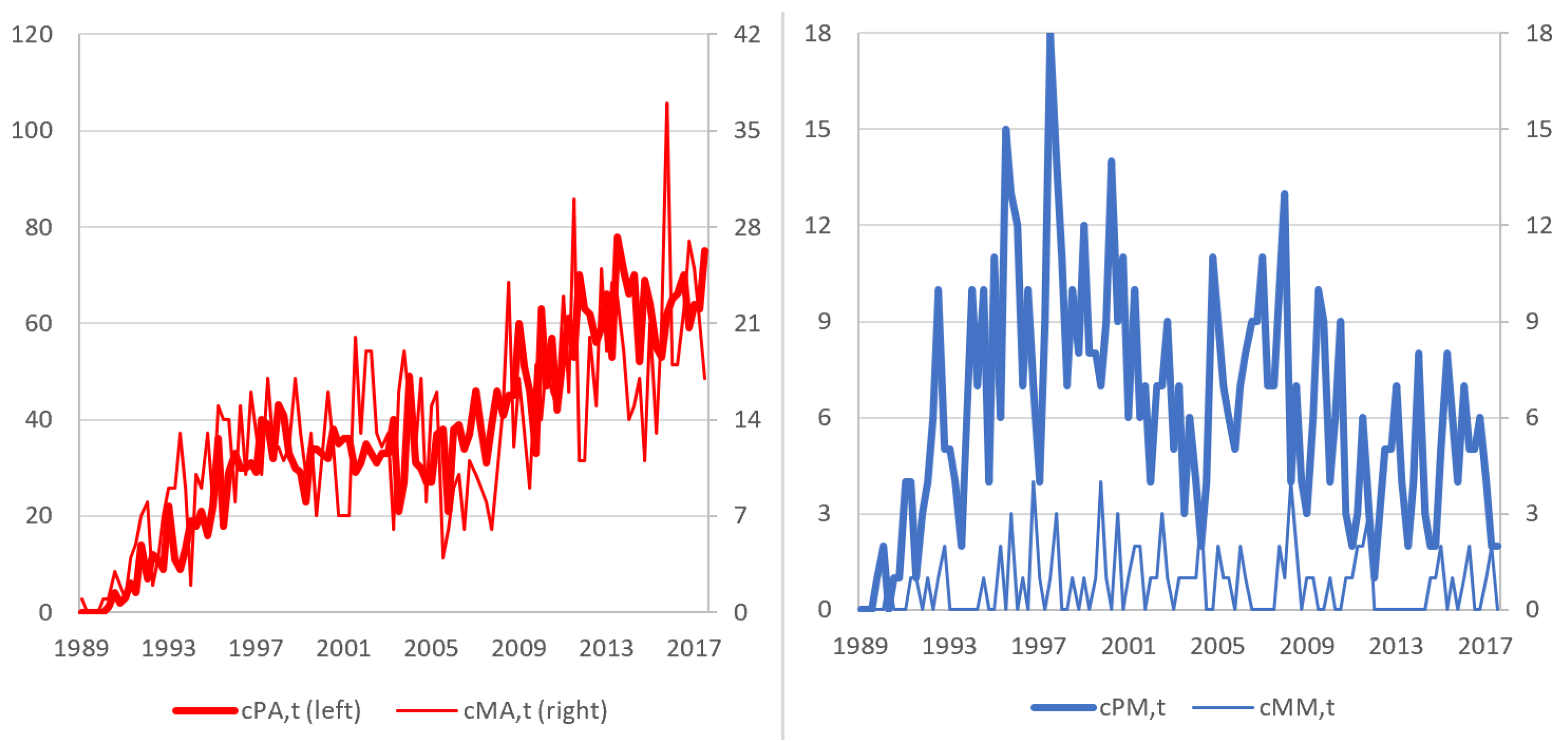
We have, therefore, derived four quarterly time series, labeled $c_{PA,t}$, $c_{MA,t}$, $c_{PM,t}$ and $c_{MM,t}$, counting the citing papers of each group in each quarter; of course, $c_t=c_{PA,t}+c_{MA,t}+c_{PM,t}+c_{MM,t}$. The four time series are reported in Figure 1, where one can observe that the behavior of $c_{PA,t}$ and $c_{MA,t}$ is quite similar, steadily increasing over time, with some low frequency fluctuations, which seem to be shared by both series (the correlation is 69.5%). Conversely, $c_{PM,t}$ has a peak around the year 2000 with about 10 papers per quarter, and then it declines until 2005, seeming to stabilize at around 5 papers per quarter. The series $c_{MM,t}$ is irregular, due to the small number of MM papers, but resembles $c_{PM,t}$ to some extent, as it shows a higher frequency around the year 2000; then, the frequency seems to slightly decline.

Finally, by combining the four series with suitable weights, we obtained two composite indicators, whose purpose is to measure the impact of KJ and SJ ideas on applied ($c_{1,t}$) and methodological ($c_{2,t}$) research:

$$\begin{array}{ccc}\hfill c_{1,t}& =& c_{PA,t}+\omega c_{MA,t}+\left(1-\omega \right)c_{MM,t}\hfill \end{array}$$

(1)

$$\begin{array}{ccc}\hfill c_{2,t}& =& c_{PM,t}+\omega c_{MM,t}+\left(1-\omega \right)c_{MA,t}\hfill \end{array}$$

(2)

Of course $c_{1,t}+c_{2,t}=c_t$for any $\omega$ by construction. Composite indicators have several pros and cons, as illustrated for example in Nardo et al. (2008) and Kuc-Czarnecka et al. (2020): they allow to summarize complex, multi-dimensional realities, reducing the dimensionality. On the other hand, they might simplify too much, and, even more importantly, the selection of indicators and weights could be the subject of dispute. It is, therefore, important to motivate clearly one’s weighting choice and to provide an extensive sensitivity analysis. We provide a thorough discussion of both aspects in Appendix B. In short, the baseline results presented in this paper are based on $\omega =0.85$. This choice is motivated by two main reasons: (i) $\omega$ should be in the range from 0.5 to 1, extremes excluded, since the papers classified as MA (or MM) should contribute mainly ($\omega >1/2$) to the applied (or methodological) index but also, to a lesser extent ($1-\omega >0$), to the methodological (or applied) index; (ii) $\omega =0.85$ would be approximately equal to $n_{PA}/(n_{PA}+n_{PM})=0.8545$—in practice, this corresponds to the assumption that the share of “applied research” of an MA paper is similar, on average, to the share of applied research in the econometric literature referring to KJ and SJ papers in general. Notice, however, that, as illustrated in Appendix B, the main results of our econometric analysis are robust to the choice of $\omega$ in the range from 0.5 to 1.

In order to fix ideas, we provide a short example based on the first few citations in the WoS data. For the year 1989, we have to split the only two existing citations by Baillie and Bollerslev (classified as MA) and Gilbert (classified as PM).7 Thus, for this example we have obtained the series illustrated in

Table 2. Illustration of the classification scheme: citations in 1989.

Author(s)	Quarter	${\mathit{c}}_{\mathit{t}}$	${\mathit{c}}_{\mathit{PA},\mathit{t}}$	${\mathit{c}}_{\mathit{MA},\mathit{t}}$	${\mathit{c}}_{\mathit{PM},\mathit{t}}$	${\mathit{c}}_{\mathit{MM},\mathit{t}}$	${\mathit{c}}_{1,\mathit{t}}$	${\mathit{c}}_{2,\mathit{t}}$
Baillie-Bollerslev	1989:Q1	1	0	1	0	0	0.85	0.15
	1989:Q2	0	0	0	0	0	0	0
	1989:Q3	0	0	0	0	0	0	0
Gilbert	1989:Q4	1	0	0	1	0	0	1

.

The cumulative applied index at time $T=115$, i.e., 2017:Q3, is equal to the following:

$$\begin{array}{ccc}\hfill C_{1,T}& =& \sum _{t=1}^T\left(c_{PA,t}+\omega c_{MA,t}+\left(1-\omega \right)c_{MM,t}\right)\hfill \\ & =& 4198+0.85\times 1451+0.15\times 92=5445.2,\hfill \end{array}$$

while the cumulative methodological index will be equal to the following:

$$\begin{array}{ccc}\hfill C_{2,T}& =& \sum _{t=1}^T\left(c_{PM,t}+\omega c_{MM,t}+\left(1-\omega \right)c_{MA,t}\right)\hfill \\ & =& 716+0.85\times 92+0.15\times 1451=1011.8.\hfill \end{array}$$

This shows that the majority of citations originates from applied research: defining $C_t=C_{1,t}+C_{2,t}$, the ratio $\frac{C_{1,T}}{C_T}$ is 84.4%, whereas $\frac{C_{2,T}}{C_T}$ is 15.6%. To check the appropriateness of our classification scheme, we analyzed how these ratios vary by publishing journal. Tracking down the 6457 citing papers, we obtained from the WoS database that they appeared in 696 distinct journals.

Table 3. The top 20 journals supplying citations to S. Johansen and K. Juselius’ works.

Rank	Journal	${\mathit{C}}_{\mathit{T}}$	$\frac{{\mathit{C}}_{1,\mathit{T}}}{{\mathit{C}}_{\mathit{T}}}$	$\frac{{\mathit{C}}_{2,\mathit{T}}}{{\mathit{C}}_{\mathit{T}}}$
1	APPLIED ECONOMICS	539	92.0%	8.0%
2	APPLIED ECONOMICS LETTERS	254	89.2%	10.8%
3	ENERGY ECONOMICS	208	94.9%	5.1%
4	ECONOMIC MODELLING	204	92.7%	7.3%
5	ENERGY POLICY	172	95.1%	4.9%
6	JOURNAL OF ECONOMETRICS	154	2.9%	97.1%
7	J. OF INTERNATIONAL MONEY & FINANCE	135	95.7%	4.3%
8	JOURNAL OF POLICY MODELING	121	96.4%	3.7%
9	ECONOMICS LETTERS	104	62.0%	38.0%
10	JOURNAL OF MACROECONOMICS	96	92.0%	8.0%
11	OXFORD BULLETIN OF ECON. & STAT.	92	46.5%	53.5%
12	ECONOMETRIC THEORY	86	0.2%	99.8%
13	EMPIRICAL ECONOMICS	81	88.6%	11.4%
14	JOURNAL OF FUTURES MARKETS	70	96.1%	3.9%
15	JOURNAL OF APPLIED ECONOMETRICS	68	54.7%	45.3%
16	MANCHESTER SCHOOL	66	94.6%	5.4%
17	ENERGY	61	92.5%	7.5%
18	JOURNAL OF BANKING & FINANCE	58	94.8%	5.2%
19	JOURNAL OF BUSINESS & ECON. STAT.	55	38.4%	61.6%
20	JOURNAL OF FORECASTING	52	51.4%	48.6%
	All Journals	6457	84.4%	15.6%

provides the ranked list of the top 20 journals by the number of citing papers: these journals hosted 2676 citing papers, i.e., 41.4%.

The evidence in Table 3 seems to confirm the validity of our classification: the average $c_{1,t}$ for the papers that appeared in mainly applied journals (for example, Energy Policy, Journal of International Money and Finance, Journal of Policy Modelling) is above 90%. To the other extreme, the average $c_{2,t}$ is above 90% for the Journal of Econometrics and for Econometric Theory (but also for Econometrica, which hosted 24 citing papers). Other journals, such as Oxford Bulletin of Economics and Statistics, Journal of Applied Econometrics, Journal of Forecasting are more balanced, with an average $c_{2,t}$ around 50%. We believe that the evidence in Table 3 supports the idea that classifying based on the title and the abstract is more accurate than classifying based on the publishing journal.

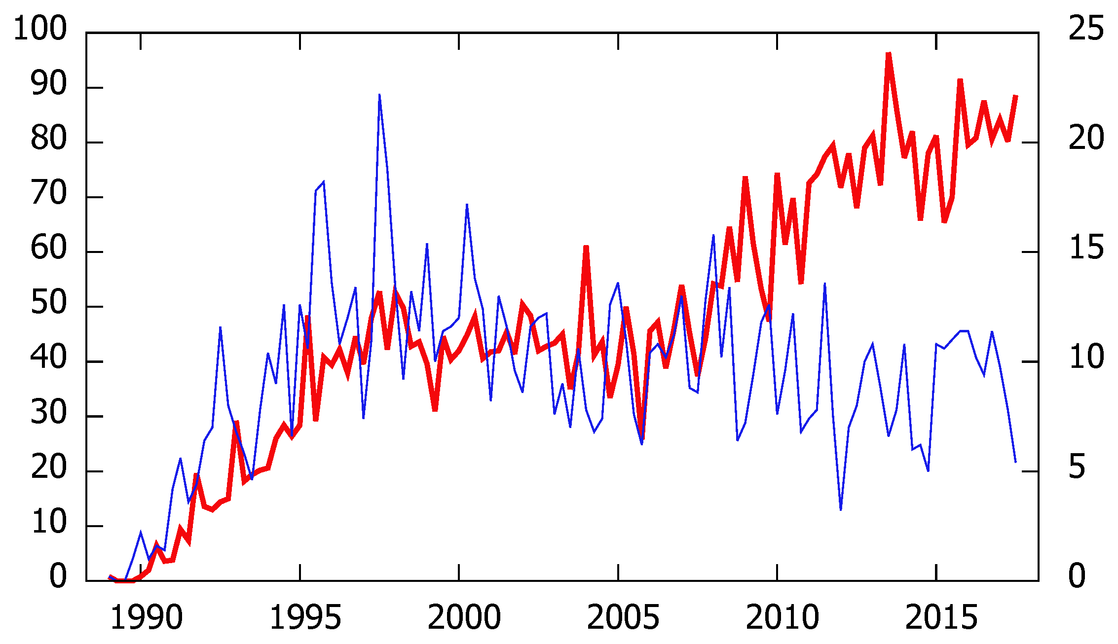
The time series $c_{1,t}$ and $c_{2,t}$ are illustrated in Figure 2. The plot shows some evidence of a “second wind” especially in the applied index $c_{1,t}$ but to some extent also in the methodological index $c_{2,t}$: both series seem to have a peak around 1998, after which they start decreasing very slowly, but around 2004 the citations start increasing again, especially for the applied research index, whereas the references found in methodological papers remain rather steady. A possibility/conjecture is that the second wind was triggered by the 2003 Nobel Prize in Economics, which popularized the concept of cointegration in a wider variety of scientific disciplines. The trajectory of $c_{1,t}$ resembles the cases of Friedrich Hayek, referred to in Bjork et al. (2014) as "bi-modal", whereas the trajectory of $c_{2,t}$ resembles more closely the cases of Kenneth Arrow and Milton Friedman, called “staying power” in Bjork et al. (2014). Boswijk et al. (2010) also claim the same with different wording: they report evidence of a “second life” for the famous Engle and Granger (1987) paper in Econometrica after the authors were awarded the Nobel prize in 2003, an event which is likely to have revamped the interest in the work of KJ and SJ as well.

3. The Bass Diffusion Model

The Bass diffusion model (Bass 1969) is widely used in many fields. Originally developed for marketing applications, the model has since been adopted also in other fields, such as the analysis of the diffusion of technological innovation (see Guseo and Guidolin 2008), bibliometric analysis (see Bjork et al. 2014) and epidemiology (see Eryarsoy et al. 2021).

The continuous time Bass model assumes a population of m potential adopters. Let us define by $t>0$ the time of adoption of a randomly picked potential adopter: t is therefore a random variable. Define by $f\left(t\right)$ the corresponding density, and by $F\left(t\right)={\int }_0^{t}f\left(u\right)du$ the cumulative density function, i.e., the probability that adoption occurs before t. Notice that the expected number of adopters at time t is given by the following:

$$\overline{C}\left(t\right)=mF\left(t\right)$$

(3)

and the corresponding “adoption intensity” is given by the following:

$$\overline{c}\left(t\right)=mf\left(t\right).$$

(4)

Bass assumes that the hazard rate $\frac{f\left(t\right)}{1-F\left(t\right)}$ is a linear function of the expected number of previous adopters:

$$\frac{f\left(t\right)}{1-F\left(t\right)}=p+qF\left(t\right),$$

(5)

where q is defined as the “imitation parameter” (or internal influence, or word-of-mouth effect) since it represents the idea that some potential adopters (imitators) tend not to adopt initially, but are more likely to adopt when the innovation is widespread. Conversely, p is defined as the “innovation parameter” (or external influence or advertising effect) since it represents the idea that some potential adopters (innovators) decide to adopt the innovation regardless of the level of diffusion. It is interesting to observe that when $q=0$, Equation (5) implies a constant hazard, and therefore the Bass model collapses into the exponential distribution. In other words, in the absence of imitators, the adoption peak, as in the exponential distribution, would occur at the beginning of the process.8

Using (3) and (4), the differential Equation (5) can be rewritten as follows:

$$\overline{c}\left(t\right)=mp+\left(q-p\right)\overline{C}\left(t\right)-\frac{q}{m}\overline{C}{\left(t\right)}^2.$$

(6)

The solution to (6) with $\overline{C}\left(0\right)=0$ is the following:

$$\overline{C}\left(t\right)=m\frac{1-e^{-\left(p+q\right)t}}{1+\frac{q}{p}{e}^{-\left(p+q\right)t}},$$

(7)

so that

$$\overline{c}\left(t\right)=\frac{\partial \overline{C}\left(t\right)}{\partial t}=m\frac{p{\left(p+q\right)}^2{e}^{-\left(p+q\right)t}}{{\left(p+q{e}^{-\left(p+q\right)t}\right)}^2}.$$

(8)

Starting from the latter equation, one can easily find the timing of the adoption peak $t^P$ (i.e., the inflection point of the diffusion curve), the corresponding peak ${\overline{c}}^P$, and the level of adoption at the peak ${\overline{C}}^P$:

$$\begin{array}{ccc}\hfill t^P& =& \frac{1}{p+q}ln\left(\frac{q}{p}\right),\hfill \end{array}$$

(9)

$$\begin{array}{ccc}\hfill {\overline{c}}^P& =& \overline{c}\left(t^P\right)=m\frac{{\left(p+q\right)}^2}{4q},\hfill \end{array}$$

(10)

$$\begin{array}{ccc}\hfill {\overline{C}}^P& =& \overline{C}\left(t^P\right)=m\frac{q-p}{2q}.\hfill \end{array}$$

(11)

Formula (9) shows that the location of the peak depends on the innovation parameter p and the imitation parameter q through the sum $\left(p+q\right)$ and the ratio $\frac{q}{p}$: as clear in Formula (5), when either innovators or imitators or both are very active so that the sum $\left(p+q\right)$ is large, then the hazard is large, which leads to a rapid exhaustion of the population at risk and therefore to an early peak.

3.1. Bass Discrete Time Model

A number of estimation procedures have been proposed to estimate the parameters m, p and q (see for example Satoh 2001). Bass (1969) suggested a simple estimation strategy based on Ordinary Least Squares (OLS) applied to a discretized version of (6) where essentially the expected adoption stock $\overline{C}\left(t\right)$ and the expected adoption flow $\overline{c}\left(t\right)$ are replaced by the observed counterpart $C_t$ and $c_t=C_t-C_{t-1}$, and an error term is added. This leads to the following:

$$c_t=mp+\left(q-p\right)C_{t-1}-\frac{q}{m}{C}_{t-1}^2+u_t.$$

(12)

In the standard discrete time Bass model, $u_t$ is assumed to be $iidN\left(0,{\sigma }^2\right)$, so that OLS is the natural candidate for estimation. To apply OLS, (12) is then reparameterized as follows:

$$c_t={\beta }_0+{\beta }_1{C}_{t-1}+{\beta }_2{C}_{t-1}^2+u_t.$$

(13)

The “reduced form” parameters $\beta ={\left({\beta }_0,{\beta }_1,{\beta }_2\right)}^{\prime }$ are related to the “structural form” parameters $\mathit{\theta }={\left(m,p,q\right)}^{\prime }$ by the following:

$$\begin{array}{ccc}\hfill {\beta }_0& =& mp,\hfill \end{array}$$

$$\begin{array}{ccc}\hfill {\beta }_1& =& q-p,\hfill \\ \hfill {\beta }_2& =& -\frac{q}{m}.\hfill \end{array}$$

(14)

and these relations can be inverted:9

$$\begin{array}{ccc}\hfill m& =& \frac{-{\beta }_1-\sqrt{{\beta }_1^2-4{\beta }_0{\beta }_2}}{2{\beta }_2},\hfill \end{array}$$

$$\begin{array}{ccc}\hfill p& =& \frac{{\beta }_0}{m}=\frac{-{\beta }_1+\sqrt{{\beta }_1^2-4{\beta }_0{\beta }_2}}{2},\hfill \\ \hfill q& =& -m{\beta }_2=\frac{{\beta }_1+\sqrt{{\beta }_1^2-4{\beta }_0{\beta }_2}}{2}.\hfill \end{array}$$

(15)

Assuming that $u_t$ is uncorrelated, homoskedastic and normal, ML estimates of the parameters vector, say $\widehat{\beta }$, can be obtained by OLS, and the corresponding variance–covariance matrix ${\widehat{\mathsf{\Sigma }}}_{\widehat{\beta }}$ can be obtained as usual.10 Replacing $\widehat{\mathit{\beta }}$ in (15) instead of $\mathit{\beta }$ gives $\widehat{\theta }=\theta \left(\widehat{\mathit{\beta }}\right)$. Defining by

$${\mathit{J}}_{\mathit{\theta }.\mathit{\beta }}=\frac{\partial \mathit{\theta }}{\partial {\mathit{\beta }}^{\prime }}$$

and using the delta method, the variance–covariance matrix associated to $\widehat{\mathit{\theta }}$ is given by the following:

$${\widehat{\mathsf{\Sigma }}}_{\widehat{\mathit{\theta }}}={\widehat{\mathit{J}}}_{\mathit{\theta }.\mathit{\beta }}{\widehat{\mathsf{\Sigma }}}_{\widehat{\mathit{\beta }}}{\widehat{\mathit{J}}}_{\mathit{\theta }.\mathit{\beta }}^{\prime },$$

(16)

where ${\widehat{\mathit{J}}}_{\mathit{\theta }.\mathit{\beta }}$ is the estimated counterpart of ${\mathit{J}}_{\mathit{\theta }.\mathit{\beta }}$. Tedious computation shows the following:

$${\mathit{J}}_{\mathit{\theta }.\mathit{\beta }}=\frac{\partial \mathit{\theta }}{\partial {\mathit{\beta }}^{\prime }}=\frac{1}{{\delta }_{\beta }}\left[\begin{array}{ccc}1& -\frac{{\beta }_1+{\delta }_{\beta }}{2{\beta }_2}& \frac{{\beta }_1\left({\beta }_1+{\delta }_{\beta }\right)-2{\beta }_0{\beta }_2}{2{\beta }_2^2}\\ -{\beta }_2& \frac{{\beta }_1-{\delta }_{\beta }}{2}& -{\beta }_0\\ -{\beta }_2& \frac{{\beta }_1+{\delta }_{\beta }}{2}& -{\beta }_0\end{array}\right],$$

(17)

where ${\delta }_{\beta }=\sqrt{{\beta }_1^2-4{\beta }_0{\beta }_2}$. ${\widehat{\mathit{J}}}_{\theta .\beta }$ is therefore obtained by replacing $\widehat{\mathit{\beta }}$ in (17).

We remark that when one considers n “seemingly unrelated” equations such as (13), i.e.,

$$c_{i,t}={\beta }_{0,i}+{\beta }_{1,i}{C}_{i,t-1}+{\beta }_{2,i}{C}_{i,t-1}^2+u_{i,t},i=1,\dots ,n,$$

(18)

and the variance–covariance matrix of ${\mathit{u}}_t={\left(u_{1,t},\dots ,u_{n,t}\right)}^{\prime }$, say ${\mathsf{\Omega }}_{\mathit{u}}$, is not diagonal, then equation by equation OLS is no longer equivalent to ML. In this case, the likelihood can be maximized by iterated Seemingly Unrelated Regression Equations (SURE), obtaining ${\widehat{\mathit{\beta }}}_i={\left({\widehat{\beta }}_{0,i},{\widehat{\beta }}_{1,i},{\widehat{\beta }}_{2,i}\right)}^{\prime }$, $i=1,\dots ,n$, ${\widehat{\mathit{\Omega }}}_{\mathit{u}}$, and the variance–covariance matrix of $\widehat{\mathit{\beta }}={\left({\widehat{\mathit{\beta }}}_1^{\prime },\dots ,{\widehat{\mathit{\beta }}}_n^{\prime }\right)}^{\prime }$, i.e.,

$${\widehat{\mathsf{\Sigma }}}_{\widehat{\mathit{\beta }}}=\left[\begin{array}{ccc}{\widehat{\mathsf{\Sigma }}}_{{\widehat{\mathit{\beta }}}_1}& \cdots & {\widehat{\mathsf{\Sigma }}}_{{\widehat{\mathit{\beta }}}_n,{\widehat{\mathit{\beta }}}_1}^{\prime }\\ ⋮& \ddots & ⋮\\ {\widehat{\mathsf{\Sigma }}}_{{\widehat{\mathit{\beta }}}_n,{\widehat{\mathit{\beta }}}_1}& \cdots & {\widehat{\mathsf{\Sigma }}}_{{\widehat{\mathit{\beta }}}_n}\end{array}\right].$$

Then, applying (15) and (16) to each pair $({\widehat{\mathit{\beta }}}_i,{\widehat{\mathsf{\Sigma }}}_{{\widehat{\beta }}_i})$ it is easy to obtain the ML estimates of the structural parameters ${\mathit{\theta }}_i={\left(m_i,p_i,q_i\right)}^{\prime }$ and the associated variance–covariance matrices.

3.2. Boswijk and Franses Model

Boswijk and Franses (2005), henceforth BF, emphasize two major problems in the model (13):

• The assumption that $u_t$ is uncorrelated is at odds with the empirical evidence that deviations of the observed adoption path with respect to the ideal equilibrium path are persistent.
• The assumption that $u_t$ is homoskedastic is disputable since, at the beginning and at the end of the diffusion process, when $c_t$ is expected to be close to zero, the variance of $c_t$ is likely to be much smaller than around the peak; related to this, simulating (13) with an homoskedastic and Gaussian error is likely to produce negative values of $c_t$ in the initial and final phases of the diffusion.

To deal with the first problem, they propose the following alternative model:11

$$\Delta c_t=\alpha \left(c_{t-1}-mp-(q-p)C_{t-1}+\frac{q}{m}{C}_{t-1}^2\right)+u_t.$$

(19)

To understand the relationship between (12) and (19) it is interesting to observe that, adding and subtracting $\alpha \left(-\left(q-p\right)C_{t-2}+\frac{q}{m}{C}_{t-2}^2\right)$ to the right hand side of (19), and rearranging, one obtains the following:

$$\Delta c_t=\alpha \left(c_{t-1}-mp-\left(q-p\right)C_{t-2}+\frac{q}{m}{C}_{t-2}^2\right)-\alpha \left(\left(q-p\right)\Delta C_{t-1}-\frac{q}{m}\Delta C_{t-1}^2\right)+u_t.$$

(20)

To interpret (20), define the following:

$$c_t^{*}=mp+\left(q-p\right)C_{t-1}-\frac{q}{m}{C}_{t-1}^2,$$

and notice that $c_t^{*}$ is the expected value or $c_t$ according to the Bass discrete time model (12). Using the notation $c_t^{*}$, (20) can be rewritten as the following:

$$\Delta c_t=\alpha \left(c_{t-1}-c_{t-1}^{*}\right)-\alpha \Delta c_t^{*}+u_t.$$

(21)

The parameter $\alpha$ is expected to be negative. The first term in (21), i.e., $\alpha \left(c_{t-1}-c_{t-1}^{*}\right)$, can be thought of as an Error-Correction Mechanism: if $c_{t-1}=c_{t-1}^{*}$, the ECM is ineffective; if instead $c_{t-1}>c_{t-1}^{*}$, then the ECM term partly corrects the disequilibrium by reducing $c_t$ with respect to $c_{t-1}$; conversely, if $c_{t-1}<c_{t-1}^{*}$, then, through the negative $\alpha$, $c_t$ will increase with respect to $c_{t-1}$. The second term in (21), i.e., $-\alpha \Delta c_t^{*}$, can be thought of as a “Target Seeking” Mechanism, which induces dynamics in $c_t$, even if $c_{t-1}=c_{t-1}^{*}$ and $u_t=0$: in fact $\Delta c_t^{*}$ will be zero when $\Delta C_{t-1}$ (and therefore $\Delta C_{t-1}^2$) is zero, which happens when the target level m is reached and therefore $C_{t-1}=C_{t-2}=m$. Another viewpoint on the BF model, seen as an AR(2) model for $C_t$ with state dependent parameters is given in Appendix A.

It is important to remark that the standard Bass model (12) is a special case of (19) with $\alpha =-1$, so that one can set up a test $H_0:\alpha =-1$ to decide which model is preferable. The interpretation of the parameters m, p and q is exactly the same in both models since (19) is a generalized version of the original Bass model, where the “adjustment intensity”, instead of being fixed at $-1$, is represented by the unrestricted parameter $\alpha$. For example, when $\alpha =-0.5$, only half of the disequilibrium observed at the end of a time unit is adjusted within the subsequent time unit: this gives rise to some persistence in the disequilibrium.

To deal with the second problem (heteroskedasticity), BF propose to model $u_t$ as the following:

$$u_t=c_{t-1}^{\varphi }{\epsilon }_t,$$

(22)

where ${\epsilon }_t$ is assumed to be uncorrelated and homoskedastic with variance ${\sigma }^2$, so that the variance of $u_t$ is assumed to be proportional to $c_{t-1}^{2\varphi }$; the authors do not consider $\varphi$ as a parameter to be estimated, but they rather fix it heuristically to either $1/2$ or 1, finding that $1/2$ is preferable in their application. In the application, we will use the residuals of the homoskedastic model to test for homoskedasticity vs. heteroskedasticity of the proposed type.

Model (19) can be reparameterized in different ways:

$$\begin{array}{ccc}\hfill \Delta c_t& =& \alpha \left(c_{t-1}-{\beta }_0-{\beta }_1{C}_{t-1}-{\beta }_2{C}_{t-1}^2\right)+u_t,\hfill \end{array}$$

(23)

$$\begin{array}{ccc}& =& \alpha c_{t-1}+{\gamma }_0+{\gamma }_1{C}_{t-1}+{\gamma }_2{C}_{t-1}^2+u_t.\hfill \end{array}$$

(24)

The parametrization (24) is suited for estimation, either with OLS when $u_t$ is assumed to be uncorrelated and homoskedastic, or by WLS (dividing left and right by $c_{t-1}^{\varphi }$), if $u_t$ is assumed to follow (22). Conversely, the parametrization (23) is useful because the parameters in $\mathit{\beta }={\left({\beta }_0,{\beta }_1,{\beta }_2\right)}^{\prime }$ are related to the parameters $\theta ={\left(m,p,q\right)}^{\prime }$ as in (15): therefore if we obtain estimates of $\mathit{\beta }$ and ${\mathsf{\Sigma }}_{\widehat{\mathit{\beta }}}$, we can map them into estimates of $\theta$ and ${\mathsf{\Sigma }}_{\widehat{\theta }}$ using (15) and (16) directly.12

Let us define ${\mathit{\gamma }}^{\prime }=\left({\gamma }_0,{\gamma }_1,{\gamma }_2\right)$. Assuming that $u_t\sim iidN\left(0,{\sigma }^2\right)$, ML estimates of ${\pi }^{\prime }=\left(\alpha ,{\mathit{\gamma }}^{\prime }\right)$ can be obtained by OLS in (24), obtaining $\widehat{\alpha }$, $\widehat{\mathit{\gamma }}$ and the corresponding variance–covariance matrix:

$${\widehat{\mathsf{\Sigma }}}_{\widehat{\mathit{\pi }}}=\left[\begin{array}{cc}{\widehat{\sigma }}_{\mathit{\alpha }}^2& {\widehat{\mathsf{\Sigma }}}_{\widehat{\mathit{\gamma }}.\widehat{\mathit{\alpha }}}^{\prime }\\ {\widehat{\mathsf{\Sigma }}}_{\widehat{\mathit{\gamma }}.\widehat{\mathit{\alpha }}}& {\widehat{\mathsf{\Sigma }}}_{\widehat{\mathit{\gamma }}}\end{array}\right].$$

Notice that $\mathit{\beta }=-\frac{1}{\alpha }\mathit{\gamma }$; therefore, ML estimates of $\mathit{\beta }$ are given by the following:

$$\widehat{\mathit{\beta }}=-\frac{1}{\widehat{\alpha }}\widehat{\mathit{\gamma }}.$$

(25)

We then obtain the following:

$${\mathit{J}}_{\mathit{\beta }.\mathit{\pi }}=\frac{\partial \mathit{\beta }}{\partial {\mathit{\pi }}^{\prime }}=\frac{1}{{\alpha }^2}\left[\begin{array}{cccc}{\gamma }_0& -\alpha & 0& 0\\ {\gamma }_1& 0& -\alpha & 0\\ {\gamma }_2& 0& 0& -\alpha \end{array}\right]=\frac{1}{{\alpha }^2}\left(\gamma ,-\alpha {\mathit{I}}_3\right),$$

and, using the delta method, we have the following:

$${\widehat{\mathsf{\Sigma }}}_{\widehat{\beta }}={\widehat{\mathit{J}}}_{\beta .\pi }{\widehat{\mathsf{\Sigma }}}_{\widehat{\pi }}{\widehat{\mathit{J}}}_{\beta .\pi }^{\prime }=\frac{1}{{\widehat{\mathit{\alpha }}}^2}\left(\frac{\widehat{\gamma }{\widehat{\gamma }}^{\prime }}{{\widehat{\mathit{\alpha }}}^2}{\widehat{\sigma }}_{\mathit{\alpha }}^2-\frac{{\widehat{\mathsf{\Sigma }}}_{\widehat{\gamma }.\widehat{\mathit{\alpha }}}{\widehat{\gamma }}^{\prime }+\widehat{\gamma }{\widehat{\mathsf{\Sigma }}}_{\widehat{\gamma }.\widehat{\mathit{\alpha }}}^{\prime }}{\widehat{\mathit{\alpha }}}+{\widehat{\mathsf{\Sigma }}}_{\widehat{\mathit{\gamma }}}\right),$$

(26)

where ${\widehat{\mathit{J}}}_{\mathit{\beta }.\mathit{\pi }}$ is the estimated counterpart of ${\mathit{J}}_{\mathit{\beta }.\mathit{\pi }}$. Starting from (25) and (26) one can obtain $\widehat{\mathit{\theta }}$ and ${\widehat{\mathsf{\Sigma }}}_{\widehat{\mathit{\theta }}}$ using (15) and (16). In particular, replacing ${\widehat{\mathsf{\Sigma }}}_{\widehat{\mathit{\beta }}}={\widehat{\mathit{J}}}_{\mathit{\beta }.\mathit{\pi }}$ ${\widehat{\mathsf{\Sigma }}}_{\widehat{\mathit{\pi }}}$ ${\widehat{\mathit{J}}}^{\prime }$ ${}_{\mathit{\beta }.\mathit{\pi }}$ in (16), one obtains the following:

$${\widehat{\mathsf{\Sigma }}}_{\widehat{\mathit{\theta }}}={\widehat{\mathit{J}}}_{\mathit{\theta }.\mathit{\beta }}{\widehat{\mathsf{\Sigma }}}_{\widehat{\mathit{\beta }}}{\widehat{\mathit{J}}}_{\mathit{\theta }.\mathit{\beta }}^{\prime }={\widehat{\mathit{J}}}_{\mathit{\theta }.\mathit{\beta }}{\widehat{\mathit{J}}}_{\mathit{\beta }.\mathit{\pi }}{\widehat{\mathsf{\Sigma }}}_{\widehat{\mathit{\pi }}}{\widehat{\mathit{J}}}_{\mathit{\beta }.\mathit{\pi }}^{\prime }{\widehat{\mathit{J}}}_{\mathit{\theta }.\mathit{\beta }}^{\prime }.$$

Additionally, in this case, when one considers n “seemingly unrelated” equations such as (24), i.e.,

$$c_{i,t}={\mathit{\alpha }}_i{c}_{i,t-1}+{\gamma }_{0,i}+{\gamma }_{1,i}{C}_{i,t-1}+{\gamma }_{2,i}{C}_{i,t-1}^2+u_{i,t},i=1,\dots ,n,$$

(27)

and the variance–covariance matrix of ${\mathit{u}}_t={\left(u_{1,t},\dots ,u_{n,t}\right)}^{\prime }$, for example ${\mathsf{\Omega }}_{\mathit{u}}$, is not diagonal, then equation by equation OLS is no longer equivalent to ML. In this case, the likelihood can be maximized by iterated SURE, obtaining ${\widehat{\mathit{\pi }}}_i={\left({\alpha }_i,{\widehat{\gamma }}_{0,i},{\widehat{\gamma }}_{1,i},{\widehat{\gamma }}_{2,i}\right)}^{\prime }$, $i=1,\dots ,n$, ${\widehat{\mathsf{\Omega }}}_{\mathit{u}}$, and the variance-covariance matrix of $\widehat{\mathit{\pi }}={\left({\widehat{\mathit{\pi }}}_1^{\prime },\dots ,{\widehat{\mathit{\pi }}}_n^{\prime }\right)}^{\prime }$, i.e.,

$${\widehat{\mathsf{\Sigma }}}_{\widehat{\mathit{\pi }}}=\left[\begin{array}{ccc}{\widehat{\mathsf{\Sigma }}}_{{\widehat{\mathit{\pi }}}_1}& \cdots & {\widehat{\mathsf{\Sigma }}}_{{\widehat{\mathit{\pi }}}_n,{\widehat{\mathit{\pi }}}_1}^{\prime }\\ ⋮& \ddots & ⋮\\ {\widehat{\mathsf{\Sigma }}}_{{\widehat{\mathit{\pi }}}_n,{\widehat{\mathit{\pi }}}_1}& \cdots & {\widehat{\mathsf{\Sigma }}}_{{\widehat{\mathit{\pi }}}_n}\end{array}\right].$$

Then, starting from each pair $\left({\widehat{\mathit{\pi }}}_i,{\widehat{\mathsf{\Sigma }}}_{{\widehat{\mathit{\pi }}}_i}\right)$ one can obtain the ML estimates of the structural parameters ${\mathit{\theta }}_i={\left(m_i,p_i,q_i\right)}^{\prime }$ and the associated variance–covariance matrices as illustrated above.

As for the asymptotic properties of ML estimates of the structural parameters, Boswijk and Franses (2005) prove that $\widehat{m}$ is consistent in T (as the time span increases $C_T$ ideally coincides with m), whereas $\widehat{p}$ and $\widehat{q}$ are not; moreover, they show that the asymptotic distribution cannot be proved to be normal. However, they demonstrate with an extensive simulation that when the frequency is allowed to go to infinity along with the time span, then $\widehat{m}$, $\widehat{p}$ and $\widehat{q}$ are essentially unbiased and asymptotically normal; they also show that this is approximately valid, even with a fixed time span, at least if it includes the inflection point $\frac{lnq-lnp}{p+q}$. In other words, if the observed time span includes the inflection point and the sampling frequency is reasonably high, their results suggest that using the standard normal and the ${\chi }^2$ for making inference on the parameters is a reasonable approximation.

3.3. Boswijk et al. Multivariate Model

Boswijk et al. (2009), henceforth BFF, propose a multivariate generalization of (19). The BFF model is made up of n equations, and can be written as follows:

$$\Delta c_{i,t}=\sum _{j=1}^n{\alpha }_{ij}\left(c_{j,t-1}-\left(p_j+q_j\right)C_{j,t-1}+\frac{q_j}{m_j}{C}_{j,t-1}^2-p_j{m}_j\right)+u_{i,t},i=1,\dots ,n,$$

(28)

where, in a simplified homoskedastic version of the model, we might assume that ${\mathit{u}}_{\mathit{t}}=\left[u_{1,t},\dots ,u_{n,t}\right]\sim iid{N}_n\left(\mathbf{0},\mathsf{\Omega }\right)$.13 Along the lines of the BF model, (28) may be reparametrized as follows:

$$\Delta c_{i,t}=\sum _{j=1}^n{\alpha }_{ij}\left({\mathit{\beta }}_j^{\prime }{X}_{j,t-1}-{\beta }_{0j}\right)+u_{it},i=1,\dots ,n,$$

(29)

with

$${\mathit{X}}_{jt}^{\prime }=\left[c_{j,t},C_{j,t},C_{j,t}^2\right],{\mathit{\beta }}_j^{\prime }=\left[1,-{\beta }_{1j},-{\beta }_{2j}\right]$$

or, more compactly,

$${\mathit{Y}}_t=\mathit{\alpha }{\mathit{\beta }}^{\prime }{\mathit{X}}_{t-1}+{\mathit{u}}_t,$$

(30)

where

$$\begin{array}{ccc}\hfill \underset{n\times 1}{{\mathit{Y}}_t}& =& \left[\begin{array}{c}\Delta c_{1,t}\\ ⋮\\ \Delta c_{n,t}\end{array}\right],\underset{\left(3n+1\right)\times 1}{{\mathit{X}}_t}=\left[\begin{array}{c}{X}_{1,t}\\ ⋮\\ X_{n,t}\\ 1\end{array}\right],\underset{n\times 1}{{\mathit{u}}_t}=\left[\begin{array}{c}{u}_{1,t}\\ ⋮\\ u_{n,t}\end{array}\right],\hfill \\ \hfill \underset{n\times n}{\mathit{\alpha }}& =& \left[\begin{array}{ccc}{\alpha }_{11}& \cdots & {\alpha }_{1n}\\ ⋮& \ddots & ⋮\\ {\alpha }_{n1}& \cdots & {\alpha }_{nn}\end{array}\right],\underset{\left(3n+1\right)\times n}{\mathit{\beta }}=\left[\begin{array}{ccc}{\mathit{\beta }}_1& \cdots & 0\\ ⋮& \ddots & ⋮\\ 0& \cdots & {\mathit{\beta }}_n\\ {\beta }_{01}& \cdots & {\beta }_{0n}\end{array}\right].\hfill \end{array}$$

Since this paper’s main goal is to celebrate Søren Johansen and Katarina Juselius, it is nice to remark that, apart from the exclusion restrictions in $\mathit{\beta }$, and the fact that the rank of $\mathit{\alpha }{\mathit{\beta }}^{\prime }$ is actually full, (30) has the mathematical form of the “reduced rank regression” popularized by Søren and Katarina; therefore, in estimating and interpreting the model, we can benefit directly from the results inspired by their work, in particular Hansen (2003). Notice that the (exclusion) restrictions on the matrix $\mathit{\beta }$ can be written as the following:

$$\mathrm{vec}\left(\mathit{\beta }\right)={\mathit{H}}_{\mathit{\beta }}{\phi }_{\mathit{\beta }}+{\mathit{h}}_{\mathit{\beta }}$$

(31)

for suitable restriction matrices ${\mathit{H}}_{\mathit{\beta }}$ and ${\mathit{h}}_{\mathit{\beta }}$.14 It might be also interesting to consider restrictions on $\mathit{\alpha }$ of the following type:

$$\mathrm{vec}\left(\mathit{\alpha }\right)={\mathit{H}}_{\mathit{\alpha }}{\phi }_{\mathit{\alpha }},$$

(32)

for example to test the hypothesis that the matrix $\mathit{\alpha }$ is diagonal, under which (28) would collapse into n “seemingly unrelated” BF equations such as (19).15 Of course, when $\mathit{\alpha }$ is unrestricted, we have that ${\mathit{H}}_{\mathit{\alpha }}={\mathit{I}}_{n^2}$ and ${\phi }_{\mathit{\alpha }}=\mathrm{vec}\left(\mathit{\alpha }\right)$.

Assuming that ${\mathit{u}}_t\sim iid\mathcal{N}\left(\mathbf{0},\mathsf{\Omega }\right)$, the log-likelihood function is given by $\ell \left(\phi ,\mathsf{\Omega }\right)=-\frac{T}{2}\left[nln\left(2\pi \right)+ln\left|\mathsf{\Omega }\right|+tr\left({\mathsf{\Omega }}^{-1}{\mathit{M}}_{uu}\right)\right]$, where ${\mathit{M}}_{uu}=T^{-1}{\sum }_{t=1}^T{\mathit{u}}_t{\mathit{u}}_t^{\prime }$. Since the log-likelihood score is bi-linear in the parameters $\mathit{\alpha }$ and $\beta$, one can employ the generalized reduced rank regression algorithm proposed by Hansen (2003) for likelihood maximization of I(1) VAR models under linear restrictions. This provides maximum likelihood estimates of the parameters $\mathit{\phi }={\left[{\mathit{\phi }}_{\mathit{\alpha }}^{\prime },{\mathit{\phi }}_{\mathit{\beta }}^{\prime }\right]}^{\prime }$ and $\mathsf{\Omega }$, for example, $\widehat{\mathit{\phi }}$ and $\widehat{\mathsf{\Omega }}$.16

To work out the variance–covariance matrix associated to $\widehat{\mathit{\phi }}$, notice that the model (30) under the restriction (31) and (32) is a sub-model of the following regression model:

$${\mathit{Y}}_t=\mathsf{\Pi }{\mathit{X}}_{t-1}+{\mathit{u}}_t,$$

where $\mathsf{\Pi }=\mathit{\alpha }{\mathit{\beta }}^{\prime }=\mathsf{\Pi }\left(\mathit{\phi }\right)$ is a smooth function of the vector of the parameters in $\mathit{\phi }$. The second derivatives of the log-likelihood with respect to $\mathrm{vec}\left(\mathsf{\Pi }\right)$ are given by $-T{\mathit{M}}_{XX}\otimes {\mathsf{\Omega }}^{-1}$, see e.g., Johansen (2006, Equation (13)), where ${\mathit{M}}_{XX}=T^{-1}{\sum }_{t=1}^T{\mathit{X}}_{t-1}{\mathit{X}}_{t-1}^{\prime }$. Because the parameters in $\mathit{\phi }$ and in $\mathsf{\Omega }$ are asymptotically independent, one finds that the Hessian with respect to $\mathit{\phi }$ equals the following:

$${\mathcal{H}}_{\mathit{\phi }}=\frac{{\partial }^2\ell \left(\mathit{\phi },\mathsf{\Omega }\right)}{\partial \mathit{\phi }\partial {\mathit{\phi }}^{\prime }}=-T{\mathit{J}}_{\mathsf{\Pi }.\mathit{\phi }}^{\prime }\left({\mathit{M}}_{XX}\otimes {\mathsf{\Omega }}^{-1}\right){\mathit{J}}_{\mathsf{\Pi }.\mathit{\phi }},$$

(33)

where

$${\mathit{J}}_{\mathsf{\Pi }.\mathit{\phi }}=\frac{\partial \mathrm{vec}\mathsf{\Pi }\left(\mathit{\phi }\right)}{\partial {\mathit{\phi }}^{\prime }}.$$

In order to describe ${\mathit{J}}_{\mathsf{\Pi }.\mathit{\phi }}$ in more detail observe that, in the present case, one has $\mathrm{vec}\mathsf{\Pi }\left(\mathit{\phi }\right)=\mathrm{vec}\mathit{\alpha }{\mathit{\beta }}^{\prime }=\left(\mathit{\beta }\otimes {\mathit{I}}_n\right)\mathrm{vec}\mathit{\alpha }=\left({\mathit{I}}_{\left(3n+1\right)}\otimes \mathit{\alpha }\right)\mathrm{vec}{\mathit{\beta }}^{\prime }$. Therefore, using (31) and (32), one finds the following:

$$\begin{array}{ccc}\hfill \partial \mathrm{vec}\left(\mathit{\alpha }{\mathit{\beta }}^{\prime }\right)/\partial {\mathit{\phi }}_{\mathit{\alpha }}^{\prime }& =& \left(\mathit{\beta }\otimes {\mathit{I}}_n\right){\mathit{H}}_{\mathit{\alpha }},\hfill \\ \hfill \partial \mathrm{vec}\left(\mathit{\alpha }{\mathit{\beta }}^{\prime }\right)/\partial {\mathit{\phi }}_{\mathit{\beta }}^{\prime }& =& \left({\mathit{I}}_{\left(3n+1\right)}\otimes \mathit{\alpha }\right){\mathcal{K}}_{\left(3n+1\right),n}{\mathit{H}}_{\mathit{\beta }}.\hfill \end{array}$$

where ${\mathcal{K}}_{mn}$ is a commutation matrix, which satisfies ${\mathcal{K}}_{mn}vec\left(\mathit{M}\right)=vec\left({\mathit{M}}^{\prime }\right)$ when $\mathit{M}$ is $m\times n$. Therefore

$${\mathit{J}}_{\mathsf{\Pi }.\mathit{\phi }}=blkdiag\left(\left(\mathit{\beta }\otimes {\mathit{I}}_n\right){\mathit{H}}_{\mathit{\alpha }},\left({\mathit{I}}_{\left(3n+1\right)}\otimes \mathit{\alpha }\right){\mathcal{K}}_{\left(3n+1\right),n}{\mathit{H}}_{\mathit{\beta }}\right).$$

The variance–covariance matrix of $\widehat{\mathit{\phi }}$ can be then estimated by the following:

$${\widehat{\mathsf{\Sigma }}}_{\widehat{\mathit{\phi }}}=-{\widehat{\mathcal{H}}}_{\mathit{\phi }}^{-1}$$

where ${\widehat{\mathcal{H}}}_{\mathit{\phi }}$ is obtained by plugging the ML estimates $\widehat{\mathit{\phi }}$ and $\widehat{\mathsf{\Omega }}$ instead of $\mathit{\phi }$ and in $\mathsf{\Omega }$ in (33).

4. Results

Our statistical analysis is based on two equations, headed to $c_{1,t}$ and $c_{2,t}$, respectively (see Section 2 for a definition of the indices). In this section, we will first discuss the estimates of the reduced form models and then the corresponding estimates of the structural form models.

4.1. Analysis of the Reduced Form—Comparing Bass, BF, BFF

As illustrated in the previous section, the two univariate Bass Equation (18) may be seen as a restricted version of the bivariate BFF model (29), with four restrictions: ${\alpha }_{11}={\alpha }_{22}=-1$ and ${\alpha }_{12}={\alpha }_{21}=0$. Similarly, the univariate dynamic BF model (27) may also be seen as a restricted version of the bivariate BFF model (29), with only two restrictions: ${\alpha }_{12}={\alpha }_{21}=0$. In all cases, assuming that the errors in the two equations are simultaneously correlated, i.e.,

$${\mathsf{\Omega }}_{\mathit{u}}=\left[\begin{array}{cc}{\sigma }_1^2& \rho {\sigma }_1{\sigma }_2\\ \rho {\sigma }_1{\sigma }_2& {\sigma }_2^2\end{array}\right],$$

efficient estimates of all models may be obtained by maximum likelihood, using the Hansen (2003) algorithm as illustrated in Section 3.3.17 The results are shown in

Table 4. ML estimates of the reduced form parameters.

		Model (18)		Model (27)		Model (29)
		Estimate	t-Ratio	Estimate	t-Ratio	Estimate	t-Ratio
APP	${\widehat{\mathit{\alpha }}}_{1,1}$	−1		−0.435	−5.74	−0.508	−6.26
	${\widehat{\mathit{\alpha }}}_{1,2}$	0		0		0.715	2.81
	${\widehat{\beta }}_{0,1}$	17.55	9.00	19.40	5.28	19.81	4.78
	${\widehat{\beta }}_{1,1}$	0.0196	9.62	0.0183	4.76	0.0190	4.61
	${\widehat{\beta }}_{2,1}$	−1.33×10${}^{-6}$	−3.22	−1.054×10${}^{-6}$	−1.35	−1.32×10${}^{-6}$	−1.60
	${\widehat{\sigma }}_1$	10.40		8.42		8.15
MET	${\widehat{\mathit{\alpha }}}_{2,1}$	0		0		0.0635	2.34
	${\widehat{\mathit{\alpha }}}_{2,2}$	−1		−0.492	−6.28	−0.547	−6.44
	${\widehat{\beta }}_{0,2}$	5.90	8.28	6.27	5.05	6.74	4.65
	${\widehat{\beta }}_{1,2}$	0.0205	5.77	0.0199	3.21	0.0187	2.73
	${\widehat{\beta }}_{2,2}$	−2.06×10${}^{-5}$	−5.71	−2.07×10${}^{-5}$	−3.29	−1.97×10${}^{-5}$	−2.86
	${\widehat{\sigma }}_2$	3.30		2.79		2.72
	$\widehat{\rho }$	0.416		0.140		0.161
	$logL$	−715.81		−682.06		−675.26

.

Table 5. Residual based tests for autocorrelation and heteroskedasticity. AC: Ljung-Box Q-statistics up to $k=20$ lags (see footnote 25 for p). HSK: Breusch–Pagan test, including the constant and $c_{1,t-1}^{2\varphi }$ (or $c_{2,t-1}^{2\varphi }$) in the regression where the dependent variable is $\frac{{\widehat{u}}_{1,t}^2}{{\widehat{\sigma }}_1^2}$ (or $\frac{{\widehat{u}}_{2,t}^2}{{\widehat{\sigma }}_2^2}$).

		Model (18)		Model (27)		Model (29)
		Test	p-Value	Test	p-Value	Test	p-Value
	$AC{\chi }_{k-p}^2$	247.3	0.000	32.64	0.013	31.74	0.016
APP	$HSK(\varphi =1/2){\chi }_1^2$	3.96	0.047	0.88	0.348	2.79	0.095
	$HSK(\varphi =1){\chi }_1^2$	3.86	0.047	0.33	0.566	1.27	0.260
	$AC{\chi }_{k-p}^2$	101.1	0.000	27.48	0.051	26.31	0.069
MET	$HSK(\varphi =1/2){\chi }_1^2$	1.41	0.235	1.77	0.184	2.96	0.085
	$HSK(\varphi =1){\chi }_1^2$	6.30	0.012	0.91	0.340	1.46	0.226

reports some misspecification tests based on the residuals illustrated in Figure 3.

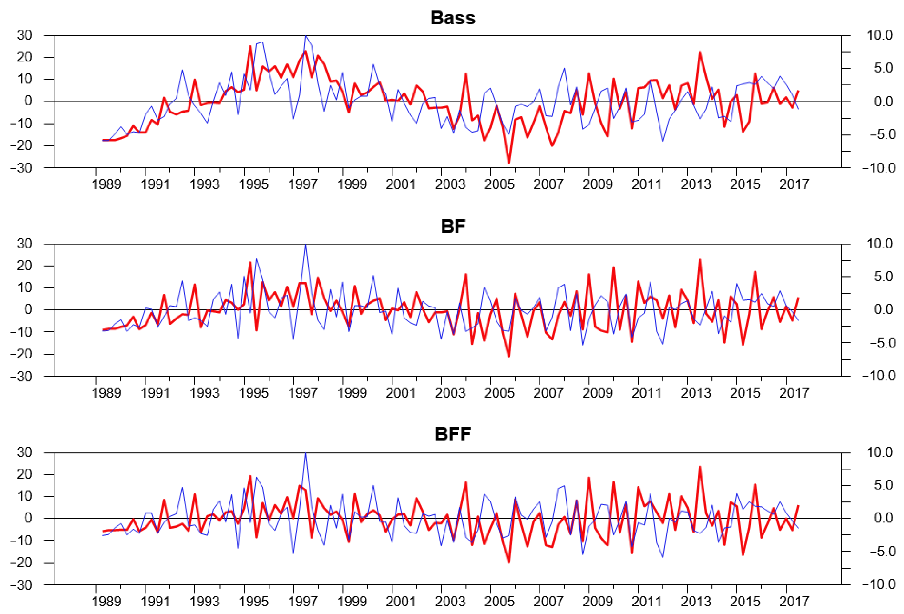
The two rows, headed AC, in the table report the results of tests for auto correlation of the residuals of the applied and methodological equation, respectively. Specifically, we tested for serial correlation up to $k=20$ lags using the Ljung-Box Q-statistic, whose null hypothesis is that the errors are uncorrelated.18 The p-value is zero for the standard Bass model (18): therefore, residuals serial correlation is a major problem for that model. Conversely, in models (27) and (29), the white noise assumption is not rejected for the methodological equation, while for the applied equation, there is a clear improvement over model (18), but some autocorrelation seems to remain for both models, which suggests to invest more on the dynamic specification, which is left for further research.

The four rows headed HSK in the table report the results of two different types of Breusch–Pagan tests for heteroskedasticity for the applied and methodological equation, respectively. In all cases, the null hypothesis is that the errors are homoskedastic, but we introduced two different alternatives. In fact, as seen in Equation (22), Boswijk and Franses (2005) suggest that the standard deviation should be proportional to $c_{i,t-1}^{\varphi }$ (with $\varphi =1/2$ or $\varphi =1$); therefore, we introduced the constant and $c_{i,t-1}^{2\varphi }$ in the auxiliary regression, with two alternative values for $\varphi$. For model (18), the null is rejected in most cases.19 Conversely, in spite of the very convincing argument supporting heteroskedasticity made by the cited authors, we did not find statistically significant evidence in this sense for this data set in (27) and (29); therefore, for the analysis in this paper, we did not consider the heteroskedastic versions of BF and BFF models.

The log-likelihood increases by $33.75$ from model (18) to model (27): the LR test is therefore ${\chi }_2^2=67.50$, and the p-value is essentially zero. According to this result, the standard Bass model seems unable to capture the persistent swings clearly visible in Figure 2 and in the first plot of Figure 3: notice in fact that both parameters ${\alpha }_{11}$ and ${\alpha }_{22}$ estimated in (27) are approximately $-0.5$ and statistically different from $-1$, which implies that only half of the distance from the ideal Bass path is corrected within one quarter, giving rise to persistent disequilibria. However, even model (27) is not satisfactory: in fact, the log-likelihood of model (29) is significantly higher (the LR test is ${\chi }_2^2=14.6$, p-value 0.00111). This result is interesting since it suggests the existence of Granger causality running from the methodological research to applied research and/or vice-versa.

To shed some light on this, we observe that the estimates of ${\mathit{\alpha }}_{12}$ and ${\mathit{\alpha }}_{21}$ in (29) are both positive and statistically significant, suggesting that an increase in the methodological research leads to expect more applications in the future, and that an increase in applications stimulates further methodological research, with a continuous dialogue between the economic problems and econometric methods, which is exactly in the spirit of KJ and SJ’s main message to the profession.

To provide a visual illustration of the relevance of the dynamic interaction between methodological and applied research in this field, we carry on a simulation exercise, similar in spirit to impulse response analysis. Impulse response functions, being the reactions of the variables to shocks entering the system, are useful for studying the interactions between variables in a vector autoregressive model (Lütkepohl 2016). In a more general non-linear setting, Potter (2000) and Koop et al. (1996) remark that nonlinear models produce impulse responses that are history- and shock-dependent; to overcome this problem, they introduce the notion of “generalized impulse response functions”, based on a stochastic simulation, which can be applied in both the linear and non-linear case. We considered this tool, but since the non-linearity is relatively mild in our case, we opted for a tailored solution that is closer to the traditional deterministic impulse response analysis.

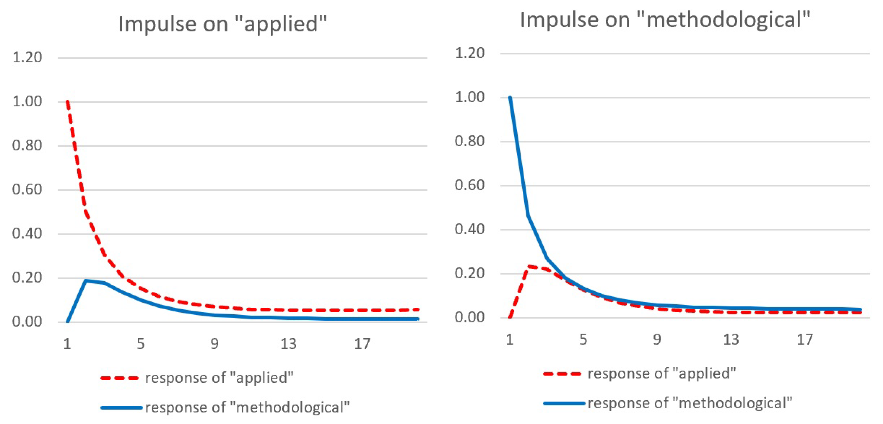
We initialize $C_{i,0}=c_{i,0}=0$,20 and then we compute two alternative trajectories for $c_{i,t}$ based on the estimated counterpart of (29). In the first dynamic simulation, $u_{i,t}$ is set to zero for all i and t: this leads to the “unshocked” paths $c_{i,t}^U$, corresponding to the deterministic trajectory that would take place in the absence on any innovation, starting from the assumed initial conditions. In the second dynamic simulation, we set $u_{j,1}={\widehat{\sigma }}_j$ in the j-th equation, whereas all other innovations (different equations and/or different times) are set to zero so that the impulse corresponds to one standard deviation in just one of the equations;21 this exercise leads to the shocked paths $c_{j,i,t}^S$, where the first subscript, j, indicates which equation has been shocked. The standardized response of the i-th equation to an impulse on the j-th equation are then given by the difference of the two trajectories, standardized by the standard deviation of the output variable as follows:

$$I{R}_{j,i,t}=\frac{\left(c_{j,i,t}^S-c_{i,t}^U\right)}{{\widehat{\sigma }}_i}j=1,\dots ,n;i=1,\dots ,n;t=1,\dots$$

The IRs therefore isolate that part of the trajectory $c_{j,i,t}^S$, which can be attributed to the shock. The first 20 IRs are illustrated in Figure 4. Notice that, by construction, $I{R}_{j,i,1}$ is equal to 1 for $j=i$, 0 otherwise. According to Figure 4, in the short run, the (standardized) response of the methodological literature to a (standardized) impulse in the applied literature appears qualitatively very similar to the (standardized) response of the applied literature to a (standardized) impulse in the methodological literature.

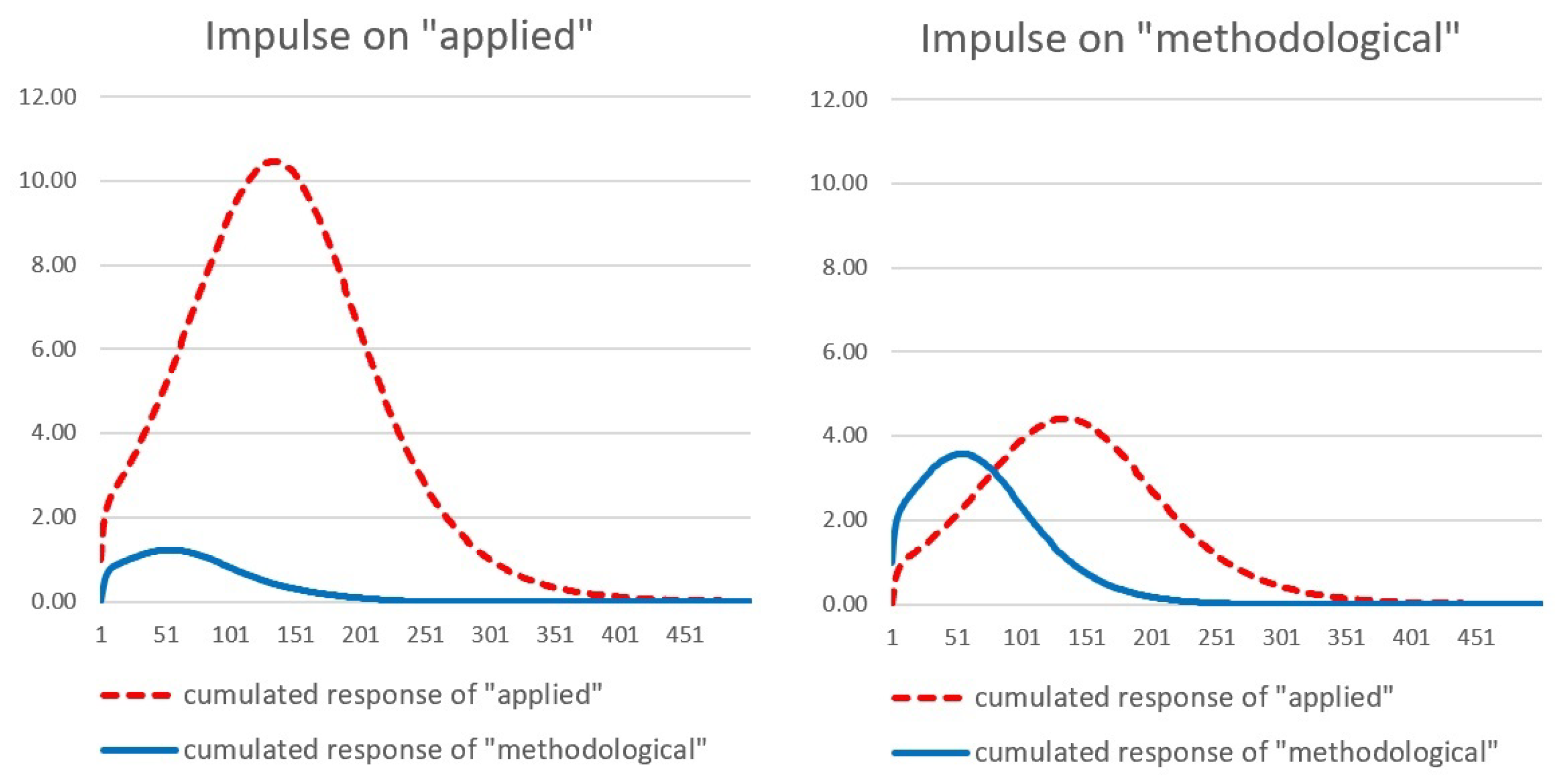
Some more insight on the relationship between methodological and applied research can be obtained by analyzing the cumulative IRs. It is important to remark that, given the mathematical nature of the model, the shocks do not have permanent effects. In fact, as t goes to infinity, the cumulative citations $C_{i,t}$ will eventually reach the saturation point $m_i$ irrespective of the initial conditions and/or the shocks they undergo: this implies that ${\sum }_{t=1}^{\infty }{c}_{i,t}^U={\sum }_{t=1}^{\infty }{c}_{j,i,t}^S=m_i-C_{i,0}$ for any i, j and $C_{i,0}$, and therefore ${\sum }_{t=1}^{\infty }I{R}_{j,i,t}=0$. As a consequence, although the first IRs illustrated in Figure 4 are positive, at some point they turn negative (although with a very small magnitude) so that, in the limit, the cumulative sum is zero. This behavior is better illustrated through the cumulative IRs, illustrated in Figure 5, for a much longer period (500 quarters).

Figure 5 shows that an impulse equal to ${\widehat{\sigma }}_1$ (i.e., 8.15 papers) in the applied literature is strongly “self exciting”, giving rise to a very long sequence of positive IRs in the applied literature itself, adding up to $10.5{\widehat{\sigma }}_1$ (about 85 papers) in the subsequent 150 quarters (almost 40 years), before it starts fading away. Conversely, the cumulative impact on the methodological literature of the same impulse is shorter living, and way less relevant ($1.2{\widehat{\sigma }}_2$, i.e., about 3 papers). On the other hand, an impulse equal to ${\widehat{\sigma }}_2$ (i.e., 2.72 papers) in the methodological literature is not so “self-exciting” (the peak of the cumulative IRs is only $3.6{\widehat{\sigma }}_2$—10 papers—about 50 quarters after the impulse), whereas the cumulative impact on the applied literature seems very important (the peak is equal to $4.4{\widehat{\sigma }}_1$—35 papers—about 150 quarters after the impulse). This evidence seems to suggest that, although in the short run, the cross fertilization is rather balanced, in the long run, the methodological literature triggers the applications more than the other way around.22

Actually, the extremely long sequence of positive IR’s, well beyond the observed period of 115 quarters, casts some doubt on the validity of the implicit assumption that the impulses do not have a permanent effect. We think that a hint for future research arising from the current study is to develop an alternative model where the saturation point $m_i$ is not already set at the beginning of the process, but it is to some extent “path dependent”. In fact, if an idea appears more successful than what was initially assumed (i.e., we observe some unexpected citations), we should reconsider the expected total number of citations in the long run, leading to an upward revision. Conversely, when an idea is suddenly abandoned, possibly in favor of an alternative paradigm (i.e., we observe an unexpected reduction in the number of citations), we should reasonably revise downwards the expected total number of citations in the long run.

4.2. Analysis of the Structural Form

Table 6. Estimates of the structural parameters of the Bass, BF and BFF models. The standard errors of the ${\widehat{t}}^P$’s measured in quarters.

		Model (12)		Model (19)		Model (28)
	Coefficient	Estimate	Std.err.	Estimate	Std.err.	Estimate	Std.err.
APP	${\widehat{m}}_1$	15,619.7	3289.6	18,332.5	9687.4	15,350.6	6396.2
	${\widehat{p}}_1$	0.00112	1.98×10${}^{-4}$	0.00106	4.79×10${}^{-4}$	0.00129	4.65×10${}^{-4}$
	${\widehat{q}}_1$	0.0207	0.00216	0.0193	0.00421	0.0203	0.00442
	${\widehat{t}}_1^P$	2022:2	16.2	2024:3	42.1	2020:4	32.4
	${\widehat{\overline{c}}}_1^P$	89	9.9	99	30.0	88	18.4
	${\widehat{\overline{C}}}_1^P$	7386	1578.9	8664	4688.9	7188	3050.6
MET	${\widehat{m}}_2$	1229.3	61.3	1212.2	100.7	1227.7	119.7
	${\widehat{p}}_2$	0.00480	5.38×10${}^{-4}$	0.00517	9.50×10${}^{-4}$	0.00549	4.91×10${}^{-4}$
	${\widehat{q}}_2$	0.0253	0.00333	0.0251	0.00580	0.0242	0.00643
	${\widehat{t}}_2^P$	2002:4	4.4	2002:1	7.2	2001:2	8.4
	${\widehat{\overline{c}}}_2^P$	11	0.5	11	0.8	11	1.0
	${\widehat{\overline{C}}}_2^P$	498	23.7	481	40.2	475	49.9

reports the “structural” parameters m, p and q in the models (12), (19) and (28), which are based on the ML estimates of (18), (27) and (29), respectively. The associated standard errors are computed using the delta method, as illustrated in Section 3.1–Section 3.3. It is important to remark that the standard errors reported for models (12) are not reliable: they appear to be much lower than in the other two models, but the assumptions for applying ML—in particular, the absence of serial correlation—are clearly invalid for that model as illustrated in Table 5.

The timing of the citations peaks ${\widehat{t}}_1^P$ and ${\widehat{t}}_2^P$, the associated peaks ${\widehat{\overline{c}}}_1^P$ and ${\widehat{\overline{c}}}_2^P$, and the corresponding cumulative number of citations at the peak ${\widehat{\overline{C}}}_1^P$ and ${\widehat{\overline{C}}}_2^P$, are obtained by plugging the estimated structural parameters in (9)–(11), and the associated standard errors are computed using the delta method.23

According to the evidence provided in Table 6, the estimates of the structural parameters are rather robust to the model used. Our comments are focused on the results based on model (28), which is statistically preferable.

It is interesting, and not surprising, that the “innovation parameter” p is much higher for the methodological literature, whereas the “imitation parameter” is quite similar in the two strands of the literature: this makes imitation relatively more important than innovation in the applied literature. As for the citation peaks, it seems that the peak in the methodological literature (11 papers per quarter) was reached in 2001, whereas the peak in the applied literature (88 papers per quarter) is expected in 2020, 12 quarters after the end of the estimation sample (although the associated standard error is extremely large—32 quarters). Based on the discussion of the properties of the estimates provided in Boswijk and Franses (2005), the estimates of the methodological equation should, therefore, be regarded as more reliable since the inflection point of the diffusion curve appears to be within the sample; this is less so for the estimates of the applied equation, where the estimated inflection point is outside the sample (of course we do not know the “true” inflection point). Not surprisingly, the standard error of ${\widehat{m}}_1$ is quite large (the coefficient of variation ${\widehat{\sigma }}_{{\widehat{m}}_1}/{\widehat{m}}_1$ is about 42%), while the standard error of ${\widehat{m}}_2$ is much smaller (the coefficient of variation ${\widehat{\sigma }}_{{\widehat{m}}_2}/{\widehat{m}}_2$ is less than 10%).

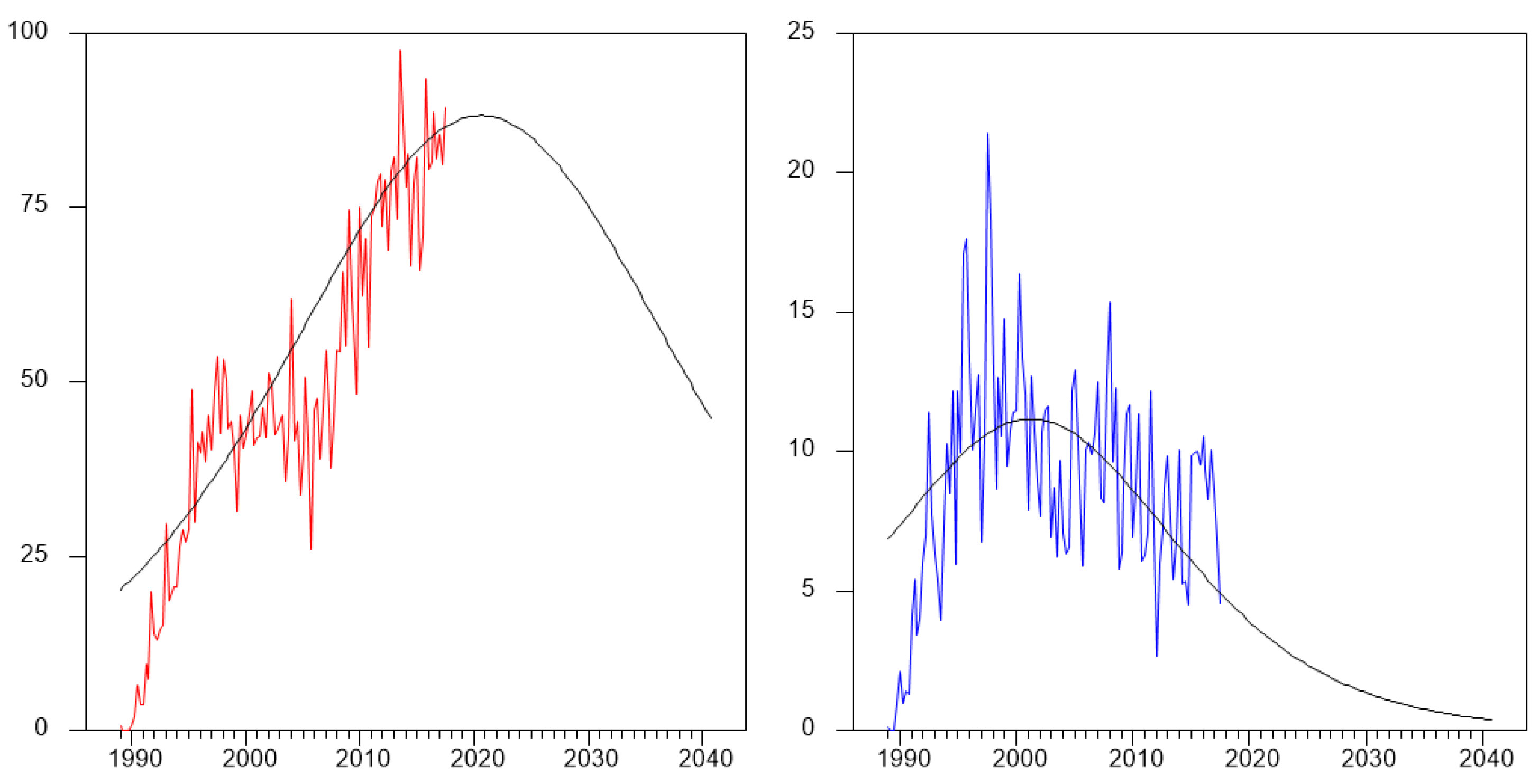
Figure 6 illustrates the observed time series along with the estimated unconditional expectation obtained by plugging the estimated structural parameters in Equation (8). Strictly speaking, since at the end of the sample (2017:Q3) we observe $C_{1,T}=5445.2$ and $C_{2,T}=1011.8$, our point estimates would ideally imply that we should expect ${\widehat{m}}_1-C_{1,T}=9905$ applied WoS papers and ${\widehat{m}}_2-C_{2,T}=216$ methodological WoS papers citing KJ and SJ in the future. We think that this interpretation is hazardous, to say the least. It is worth observing that the estimates of the structural parameters, especially $m_1$ and $m_2$, are very unstable as observed among others in Chandrasekaran and Tellis (2018), and they mainly seem to represent the history of the process in a descriptive sense rather than being a reliable forecasting tool in an inferential sense. For example, if we re-estimate the parameters based on the sub sample 1989:Q1-2005:Q4, so that the end of the sample occurs right before the “second wind” clearly visible in the plot, we would obtain ${\widehat{m}}_1=2710.6$ (${\widehat{\sigma }}_{{\widehat{m}}_1}=142.5$), ${\widehat{m}}_2=684.3$ (${\widehat{\sigma }}_{{\widehat{m}}_2}=34.7$), ${\widehat{t}}_1^P=$1999:Q1 and ${\widehat{t}}_2^P=$1997:Q4.24 Therefore, estimating the same model 15 years ago, one would be convinced of the following: (i) that the citations peak was already reached several years before (and then the estimates would be regarded as reliable); (ii) that the potential for this literature was about one fifth of what it appears now; and (iii) that by 2020, the interest in KJ and SJ work will have disappeared (see Figure 7). However, as this Special Issue confirms, no prediction could have proved more wrong!

5. Conclusions and Suggestions for Further Research

Our main purpose in writing this paper was to contribute to the Festschrift in honor of Katarina Juselius and Søren Johansen as a sign of gratitude for their being for us a constant source of inspiration. We tried to find a way to show how profoundly they contributed to the development of economic ideas, emphasizing one key aspect of their approach, namely, the dialogue between empirical economics and econometric methodology. To this aim, we have proposed an operational way to disentangle, as much as possible, their contribution to applied and methodological econometric research, through the development of two indices based on the Web of Science database. We hope that this can also be a contribution to bibliometric studies since a similar approach to assess in a quantitative way the impact of new ideas on methodological and applied research, and on the interaction between them, can be used for other areas. Ideally, similar analyses might be employed to investigate even more general epistemological issues, such as the relationship between theoretical and empirical research.

We think that the data we describe in Section 2 are very interesting per se. They show that KJ and SJ’s influence on the literature is extremely important: their top 10 papers sum up to about 10,500 WoS citations (more than 50,000 in GS) from about 6500 citing papers, an average of more than 200 papers per year. Based on our indicators, 85% of the citing papers are essentially applied, whereas 15% are methodological: we do not have a benchmark for comparison, but we have the impression that the share of methodology is somewhat larger than in the econometric literature in general. As of 2017, the number of applied citing papers per quarter had not yet reached the peak (although a “false peak” seems to have occurred around 2000); conversely, the peak in the methodological literature seems to have been reached around 2001, although the shape of the trajectory is very flat after the peak, similar to what Bjork et al. (2014) has identified in a minority of Nobel prize winners and defined as “staying power”.

To model the data, we resorted to an innovative dynamic multivariate version—proposed in Boswijk et al. (2009)—of the well-known Bass (1969) model. It was a pleasure for us to observe and emphasize that this model resembles so closely the Vector ECM model popularized by KJ and SJ; in particular, the bilinear nature of the model allows to use the Hansen (2003) algorithm to maximize the likelihood, which generalizes Johansen’s ML algorithm, adapting it to a rather general class of restrictions, which includes our case.

The estimated model conveys very interesting information. As seen in Formula (9), the location of the citations peaks depends on the relative importance of the “innovation parameter” p and the “imitation parameter” q. Our estimates suggest that the different location of the peaks might be explained by the higher value of the parameter $q_2$ with respect to $q_1$, whereas $p_1$ and $p_2$ are quite similar: using the standard terminology in the Bass model literature, the difference in the parameters suggests that the methodological literature is mainly driven by “innovators”, whereas “imitators” are relatively more important in the applied literature.

Another interesting finding is that, in the literature referring to KJ and SJ, the “cross-fertilization” between methodological and applied research is statistically significant and bi-directional (although possibly more effective from methodology to applications than the other way round). According to our impulse response analysis, rounding our figures, 8 unexpected applied papers in one quarter lead to predict that 3 methodological papers will follow, whereas 3 unexpected methodological papers lead to predict that 40 applied papers will follow (this is not so unbalanced as it seems at first sight since the scale of the two strands of literature is different). These results testify that one of the most important messages that Katarina Juselius and Søren Johansen have emphasized in their writings—i.e., that the applications should pose challenging problems to the methodology and that the methodology should sharpen the ability of applied researchers to ask meaningful questions to the data—has become a common heritage in this literature.

As for the estimated dimension of KJ and SJ influence, as measured by the parameters $m_1$ and $m_2$ (often called “saturation point” or “ceiling”), a word of caution is in order. Our estimates, ${\widehat{m}}_1$ = 15,351 and ${\widehat{m}}_2=1228$, imply that we should expect about 10,000 applied WoS papers and 200 methodological WoS papers citing KJ and SJ in the future. We do not consider these figures very reliable. Indeed, early in the literature, it was pointed out by Heeler and Hustad (1980) and others (e.g., Hyman 1988) that the predicting ability of the Bass model depends on the generation of accurate estimates of m. Srinivasan and Mason (1986) report problems with convergence when the data set does not contain the peak time period (i.e., the inflection point of the curve). The parameter m is, again, under attack in Van den Bulte and Lilien (1997): there is evidence of downward bias in the estimation of the saturation point. Finally, in their review article Chandrasekaran and Tellis (2018), point out the overall poor forecasting ability, the unstable parameter estimates and the difficulty to define a clear stopping rule for the time window regarding data collection for the Bass model (since the data should, in theory, end when the entire market has adopted). We add one more critique to the list: the parameter m, in the logic of the Bass model, appears to be in the DNA of the process since the onset and to be immutable over time. In all versions of the model that we have considered, the “shocks” (i.e., the unexpected citing papers) have no permanent effect in the sense that they determine, at most, a persistent (but transitory) departure from a path, which eventually leads to m. In the spirit of the unit roots literature, so much inspired by the contribution of Katarina Juselius and Søren Johansen, our suggestion for further methodological research is to try and conceive a new model, where the shocks are allowed to have a permanent effect on the “ceiling”. We think that this is absolutely needed in the applications, such as the bibliometric ones, where the notion of “population at risk” or “potential” is not obvious. However, also in marketing, or epidemiology, or in the analysis of technological innovation, the final diffusion is likely to be influenced in a crucial way by events that are largely unpredictable; therefore, pretending that the same differential equation—where m is fixed since $t=0$—drives the dynamics of the process along its entire history might not be a realistic representation of the observed phenomena.

References

- Bass, Frank M. 1969. A new product growth for model consumer durables. Management Science 15: 215–27. [Google Scholar] [CrossRef]
- Bjork, Samuel, Avner Offer, and Gabriel Söderberg. 2014. Time series citation data: The nobel prize in economics. Scientometrics 98: 185–96. [Google Scholar] [CrossRef]
- Boswijk, H. Peter, Dennis Fok, and Philip Hans Franses. 2009. A New Multivariate Product Growth Model. Amsterdam: University of Amsterdam, Technical Report, Econometrics Discussion Paper 2009/07. [Google Scholar]
- Boswijk, H. Peter, and Philip Hans Franses. 2005. On the econometrics of the bass diffusion model. Journal of Business & Economic Statistics 23: 255–68. [Google Scholar] [CrossRef] [Green Version]
- Boswijk, H. Peter, Philip Hans Franses, and Dick van Dijk. 2010. Cointegration in a historical perspective. Journal of Econometrics 158: 156–59. [Google Scholar] [CrossRef] [Green Version]
- Chandrasekaran, Deepa, and Gerard J. Tellis. 2018. A Summary and Review of New Product Diffusion Models and Key Findings. chapter 14. Cheltenham: Edward Elgar Publishing, pp. 291–312. [Google Scholar] [CrossRef]
- Coupé, Tom. 2003. Revealed performances: Worldwide rankings of economists and economics departments, 1990–2000. Journal of the European Economic Association 1: 1309–45. [Google Scholar] [CrossRef]
- Engle, Robert F., and Clive W. J. Granger. 1987. Co-integration and error correction: Representation, estimation, and testing. Econometrica 55: 251–71. [Google Scholar] [CrossRef]
- Eryarsoy, Enes, Dursun Delen, Behrooz Davazdahemami, and Kazim Topuz. 2021. A novel diffusion-based model for estimating cases, and fatalities in epidemics: The case of covid-19. Journal of Business Research 124: 163–87. [Google Scholar] [CrossRef]
- Fok, Dennis, and Philip Hans Franses. 2007. Modeling the diffusion of scientific publications. Journal of Econometrics 139: 376–90. [Google Scholar] [CrossRef] [Green Version]
- Franses, Philip Hans. 2003. The diffusion of scientific publications: The case of econometrica, 1987. Scientometrics 56: 29–42. [Google Scholar] [CrossRef]
- Garfield, Eugene, Morton V. Malin, and Henry Small. 1978. Citation data as science indicators. In Toward a Metric of Science: The Advent of Science Indicators. Edited by Yehuda Elkana, Joshua Lederberg, Robert K. Merton, Arnold Thackray and Harriet Zuckerman. New York: John Wiley & Sons, pp. 179–207. [Google Scholar]
- Guseo, Renato, and Mariangela Guidolin. 2008. Cellular automata and riccati equation models for diffusion of innovations. Statistical Methods and Applications 17: 291–308. [Google Scholar] [CrossRef]
- Hansen, Peter Reinhard. 2003. Structural changes in the cointegrated vector autoregressive model. Journal of Econometrics 114: 261–95. [Google Scholar] [CrossRef] [Green Version]
- Heeler, Roger M., and Thomas P. Hustad. 1980. Problems in predicting new product growth for consumer durables. Management Science 26: 1007–20. [Google Scholar] [CrossRef]
- Hendry, David, and Katarina Juselius. 2001. Explaining cointegration analysis. part ii. The Energy Journal 22: 75–120. [Google Scholar] [CrossRef] [Green Version]
- Hyman, Michael R. 1988. The timeliness problem in the application of bass-type new product-growth models to durable sales forecasting. Journal of Business Research 16: 31–47. [Google Scholar] [CrossRef]
- Johansen, Søren. 1988. Statistical analysis of cointegration vectors. Journal of Economic Dynamics and Control 12: 231–54. [Google Scholar] [CrossRef]
- Johansen, Søren. 1991. Estimation and hypothesis testing of cointegration vectors in gaussian vector autoregressive models. Econometrica 59: 1551–80. [Google Scholar] [CrossRef]
- Johansen, Søren. 1992a. Cointegration in partial systems and the efficiency of single-equation analysis. Journal of Econometrics 52: 389–402. [Google Scholar] [CrossRef]
- Johansen, Søren. 1992b. Determination of cointegration rank in the presence of a linear trend. Oxford Bulletin of Economics and Statistics 54: 383–97. [Google Scholar] [CrossRef]
- Johansen, Søren. 1992c. Testing weak exogeneity and the order of cointegration in uk money demand data. Journal of Policy Modeling 14: 313–34. [Google Scholar] [CrossRef]
- Johansen, Søren. 1995. Likelihood-Based Inference in Cointegrated Vector Autoregressive Models. Oxford: Oxford University Press. [Google Scholar] [CrossRef]
- Johansen, Søren. 2006. Statistical analysis of hypotheses on the cointegrating relations in the i(2) model. Journal of Econometrics 132: 81–115. [Google Scholar] [CrossRef]
- Johansen, Søren, and Katarina Juselius. 1990. Maximum likelihood estimation and inference on cointegration—With applications to the demand for money. Oxford Bulletin of Economics and Statistics 52: 169–210. [Google Scholar] [CrossRef]
- Johansen, Søren, and Katarina Juselius. 1992. Testing structural hypotheses in a multivariate cointegration analysis of the ppp and the uip for uk. Journal of Econometrics 53: 211–44. [Google Scholar] [CrossRef]
- Johansen, Søren, and Katarina Juselius. 1994. Identification of the long-run and the short-run structure an application to the islm model. Journal of Econometrics 63: 7–36. [Google Scholar] [CrossRef]
- Johansen, Søren, Rocco Mosconi, and Bent Nielsen. 2000. Cointegration analysis in the presence of structural breaks in the deterministic trend. The Econometrics Journal 3: 216–49. [Google Scholar] [CrossRef] [Green Version]
- Juselius, Katarina. 2006. The Cointegrated VAR Model: Methodology and Applications. Oxford: Oxford University Press. [Google Scholar]
- Juselius, Katarina. 2021. Searching for a theory that fits the data: A personal research odyssey. Econometrics 9: 5. [Google Scholar] [CrossRef]
- Kalaitzidakis, Pantelis, Theofanis P. Mamuneas, and Thanasis Stengos. 1999. European economics: An analysis based on publications in the core journals. European Economic Review 43: 1150–68. [Google Scholar] [CrossRef]
- Kalaitzidakis, Pantelis, Theofanis P. Mamuneas, and Thanasis Stengos. 2003. Rankings of academic journals and institutions in economics. Journal of the European Economic Association 1: 1346–66. [Google Scholar] [CrossRef] [Green Version]
- Katsaliaki, Korina, and Navonil Mustafee. 2011. Applications of simulation within the healthcare context. Journal of the Operational Research Society 62: 1431–51. [Google Scholar] [CrossRef]
- Koop, Gary, M. Hashem Pesaran, and Simon M. Potter. 1996. Impulse response analysis in nonlinear multivariate models. Journal of Econometrics 74: 119–47. [Google Scholar] [CrossRef]
- Kuc-Czarnecka, Marta, Samuele Lo Piano, and Saltelli Andrea. 2020. Quantitative storytelling in the making of a composite indicator. Social Indicators Research 1: 775–802. [Google Scholar] [CrossRef] [Green Version]
- Lütkepohl, Helmut. 2016. Impulse Response Function. London: Palgrave Macmillan UK, pp. 1–5. [Google Scholar] [CrossRef]
- Min, Chao, Ying Ding, Jiang Li, Yi Bu, Lei Pei, and Jianjun Sun. 2018. Innovation or imitation: The diffusion of citations. Journal of the Association for Information Science and Technology 69: 1271–82. [Google Scholar] [CrossRef]
- Nardo, Michela, Michaela Saisana, Andrea Saltelli, Stefano Tarantola, Anders Hoffmann, and Enrico Giovannini. 2008. Handbook on Constructing Composite Indicators: Methodology and User Guide. Paris: OECD Publishing. [Google Scholar]
- Pesaran, H. Hashem, and Yongcheol Shin. 1998. Generalized impulse response analysis in linear multivariate models. Economics Letters 58: 17–29. [Google Scholar] [CrossRef]
- Potter, Simon M. 2000. Nonlinear impulse response functions. Journal of Economic Dynamics and Control 24: 1425–46. [Google Scholar] [CrossRef] [Green Version]
- Redner, Sidney. 1998. How popular is your paper? An empirical study of the citation distribution. The European Physical Journal B-Condensed Matter and Complex Systems 4: 131–34. [Google Scholar] [CrossRef]
- Satoh, Daisuke. 2001. A discrete bass model and its parameter estimation. Journal of the Operations Research Society of Japan 44: 1–18. [Google Scholar] [CrossRef] [Green Version]
- Srinivasan, V., and Charlotte H. Mason. 1986. Nonlinear least squares estimation of new product diffusion models. Marketing Science 5: 169–78. [Google Scholar] [CrossRef] [Green Version]
- Stigler, Stephen M. 1994. Citation patterns in the journals of statistics and probability. Statistical Science 9: 94–108. [Google Scholar] [CrossRef]
- Stokes, Donald E. 1997. Pasteur’s Quadrant: Basic Science and Technological Innovation. Washington: Brookings Institution Press. [Google Scholar]
- Van den Bulte, Christophe, and Gary L. Lilien. 1997. Bias and systematic change in the parameter estimates of macro-level diffusion models. Marketing Science 16: 338–53. [Google Scholar] [CrossRef]
- Vieira, Pedro, and Aurora Teixeira. 2010. Are finance, management, and marketing autonomous fields of scientific research? An analysis based on journal citations. Scientometrics 85: 627–46. [Google Scholar] [CrossRef] [Green Version]
- Zitt, Michel. 2006. Scientometric indicators: A few challenges. data mine-clearing; knowledge flows measurements; diversity issues. Invited plenary talk. Paper presented at the International Workshop on Webometrics, Informetrics and Scientometrics & Seventh COLLNET Meeting, Nancy, France, December 12–15. [Google Scholar]
Figure 1.
Time series plot of , , and , quarterly data from 1989:1 to 2017:3.
Figure 2.
The composite citation indices (thick red, left scale) and (thin blue, right scale), quarterly data from 1989:1 to 2017:3.
Figure 3.
Residuals of different models: Bass = model (18), BF = model (27), BFF = model (29). Thick red line = “Applied” (left scale). Thin blue line = “Methodological” (right scale).
Figure 4.
Standardized impulse responses based on model (29). Initialization: , .
Figure 5.
Cumulative standardized impulse responses based on model (29). Initialization: , .
Figure 6.
Observed time series along with the estimated unconditional expectation based on Equation (8). Left—applied index; right—methodological index.
Figure 7.
Forecasting fallacy: observed time series along with the estimated unconditional expectation based on (8), parameters re-estimated based on the trimmed sample 1898:Q1-2005:Q4. Left—applied index; right—methodological index.