Spatial Patterns in Fiscal Impacts of Environmental Taxation in the EU

Abstract

There are several reasons for environmental taxation implementation. Besides its environmental impact, the main reason for such taxation is its fiscal impact, particularly in generating revenues of public budgets. The main goal of this paper is to observe possible spatial patterns in fiscal impacts of environmental taxation in the EU countries, and to depict the groups of countries with the same (or similar) fiscal impact of these instruments on public budget revenues, including environmental and economic characteristics. Two methods of cluster analysis are used, Ward linkage and K-nearest neighbors (spatial) cluster analysis to observe potential geographical links or implication of fiscal impact. The study is performed for the years 2008 and 2017. Based on the results, we can say that in the year 2008, the EU countries were divided into “the west” and “the east”, with some exceptions. The western countries were characterized by high environmental tax revenues, the eastern countries by low environmental tax revenues. For 2017, the situation is different. The border between old and new EU member states is not so abrupt and clear. The results show higher diversification between EU countries concerning the fiscal impacts of environmental taxation.

1. Introduction

Currently, raising revenues and addressing climate change are two fundamental challenges facing governments (Barrage 2020). The European Union (EU) member states use various economic instruments of environmental/climate protection. The range of instruments includes, among others, environmental taxes, fees, charges, tradable permits, deposit-refund systems and subsidies (Eurostat 2013; European Commission 2016). Environmental taxes should play an essential part in environmental policy as they help to internalize externalities, reduce damage and increase the quality of life; they also allow for the raising of revenue for national and local governments (Jurušs and Brizga 2017). Therefore, besides their environmental impact, the main reason for these economic instruments’ implementation is their fiscal impact—namely, the revenues of public budgets (OECD 2016).

The EU has increasingly favored such instruments because they provide flexible and cost-effective means of reinforcing the polluter-pays principle and for reaching environmental policy objectives (Hájek et al. 2019). Regarding environmental taxation, Eurostat (2013) distinguishes four categories of environmental taxes: energy taxes (including fuel for transport), transport taxes, pollution taxes and resource taxes. Government revenues from the auctioning of emission permits are treated as tax receipts in the national accounts; therefore, they are part of the energy taxes (Eurostat 2013; European Commission 2016).

Since environmental taxation represents the additional revenues of state/public budgets, the questions might emerge: what is the level of economic burden connected with environmental tax policy in particular EU member states? Are there any common features and trends between countries or groups of countries?

Concerning practically significant studies in this field we can generally divide them into studies focusing on environmental impacts and studies focusing on the fiscal impacts of such taxation. Recent scientific studies in the field of environmental impacts of environmental taxation are mainly case studies for specific countries. A case study of Spain (Gemechu et al. 2014) included an analysis of direct and indirect effects of an environmental tax imposed on Spanish products, using environmental input-output (EIO) and price models. Pereira and Pereira (2014) studied CO₂ taxation in its dual role as a climate and a fiscal policy instrument in Portugal. They developed marginal abatement cost curves for CO₂ emissions associated with CO₂ tax using a dynamic general equilibrium model of the Portuguese economy. Solaymani (2017) focused on carbon and energy taxation in Malaysia. Heerden et al. (2016) analyzed the economic and environmental effects of the carbon tax in South Africa, using the dynamic CGE modelling approach. Jurušs and Brizga (2017) assessed the role of environmental taxes used in Latvia’s environmental policy, using desk research. Frey (2017) evaluated the impact of different carbon tax levels on the Ukrainian economy and the environment, observing evidence for a robust double dividend. Hájek et al. (2019) analyzed carbon tax efficiency in the energy industries of selected EU countries, finding out that carbon tax is more effective than CO₂ emission trading in these countries.

Dealing with fiscal impacts of environmental taxation, it is worth mentioning the recent research of Barrage (2020), who studied the optimal design of carbon taxes both as an instrument to control climate change and as a part of fiscal policy. Based on the results, the imposition of appropriately designed carbon taxes could yield substantial benefits, both in terms of raising revenues and by significantly improving intertemporal production efficiency. Labandeira et al. (2019) analyzed the possibilities of new green tax reforms, as a consequence of an increased need for public revenues. Their study explores the possibilities of implementing a new generation of green tax reforms in Spain, focusing on various impacts, including public revenues and income distribution from taxing various energy-related environmental damages and by considering fiscal consolidation and funding the costs of renewable energy support schemes.

There are not many studies focusing on the spatial aspect of environmental taxation in this field. For example, Xiangmei and Yang (2018) analyzed spatial issues in China, observing temporal and spatial distribution characteristics of the air pollution index (API) and its correlation with the improvement of environmental tax law. Their paper discussed the general trend of the China air pollution index and studied the daily air pollution index of important cities focusing on the three dimensions of time, space, and trend. For analyzing the relationship of API with environmental tax laws, the authors used methods of studying regional differences in the economic discipline, especially the Searl index. The discussion underlines the topic of how to allocate resources in the redistribution of tax rationally.

Other research papers dealing with spatial aspects carry out firm responses to a carbon price and corporate decision making under British Columbia’s (BC) carbon tax (Bumpus 2015). The research is empirical and focuses on firms, which experienced difficulty in making low-carbon changes in response to fluctuating commodity prices, the low certainty of climate policy over temporal and spatial scales and the political economy of implementing regional climate policy. The study presents the results of empirical research of industry participation, and interviews with executives of major emitting firms in BC.

Concerning both fiscal aspects and spatial distribution of environmental taxation, using cluster analysis as a methodological approach, there is a lack of such scientific studies. There are some excise taxation studies, which are close to the environmental topic. For example, Lin and Wen (2012) carry out an analysis of temporal changes in geographical disparities in alcohol-attributed disease mortality (ADM) before and after implementation of the alcohol tax policy in Taiwan. As a methodological approach, they used local spatial statistical methods to explore the geographic variations in ADM rates and identify statistically significant clusters among townships. Then, we can find studies observing spatial patterns in various taxation issues in European countries, as well. For example, Zaharia et al. (2017) focused on the environmental taxation in EU countries and the comparison of clusters in the year 2002 with the year 2012, using Ward linkage cluster analysis. Another study, Liapis et al. (2013), provided clusters of economic similarities between EU countries, calculating with different categories of economic indicators, including tax revenues. However, this analysis does not include all EU countries and the environmental tax revenues are not included in the category “tax revenues”. Stuhlmacher et al. (2019) performed a systematic, spatial-economic assessment of the EU ETS. They analyzed the spatial pattern of emissions changes using clustering analysis of emissions changes at the EU and country-level in the period 2005–2012. Pászto and Zimmermannová (2019) evaluated the development of CO₂ emissions and selected economic indicators of EU-28 countries in the period from 2005 to 2015, capturing the geographical patterns and spatial distribution of countries emitting pollution. Skovgaard et al. (2019) explored patterns of adoption (both implemented policies and those scheduled to be) through cluster analysis to investigate factors that could explain policies’ decisions to adopt carbon pricing. The study contributed empirically by studying carbon taxes and emissions trading together and by clustering the polities adopting carbon pricing.

Currently, there is no such spatial analysis of the fiscal aspects of environmental taxation in EU countries, observing (Central and Eastern Europe) CEE countries in more detail and simultaneously taking EU ETS state budget revenues as a separate category. Moreover, the above-mentioned scientific studies use only one method of cluster analysis—Ward’s or K-nearest neighbors’ method. Focusing on this gap in the scientific field, we carry out the following research.

The main goal of this paper is (1) to observe possible spatial patterns in fiscal impacts of environmental taxation in EU countries, with a focus on CEE countries (comprising of Albania, Bulgaria, Croatia, Czechia, Hungary, Poland, Romania, Slovakia, Slovenia, and the three Baltic States: Estonia, Latvia and Lithuania (OECD 2019), and (2) to depict the groups of countries with the same (or similar) fiscal impact of these instruments on public budget revenues, including environmental and economic characteristics of analyzed countries.

As an input motivation to our research, we were inspired by the EU document (European Commission 2019) underlining consequences with environmental taxation: “In general, two groups of Member States can be distinguished: (1) A group of "low-taxing Member States". These are typically taxing at rates close to the minima and have often, although not in all cases, introduced taxation only as a consequence of the existence of common minimum rates. Many of the new Member States are in this group (Slovenia is one exception); (2) A group of "high-taxing Member States" with tax levels more or less clearly above the minima. For these countries, the existence of common minima is particularly important to reduce competitive disadvantages for their industry. These countries also often make use of the possibility to apply reduced rates for energy-intensive businesses. The Nordic countries are among the highest taxing Member States, especially for heating fuels”.

Concerning this document, our research focuses on observing characteristics of environmental tax revenues in EU countries to find possible groups of them. The following research questions are defined:

(1) Can we observe similar characteristics between Central and Eastern Europe (CEE) countries, as representants of a group of “low-taxing Member States”?

(2) Can we observe any spatial-temporal changes in groups of countries in general (focusing on the years 2008 and 2017)?

Given the lack of studies focusing on spatial patterns of the environmental taxation, the authors will examine and evaluate (1) possible geographical patterns in the revenues of the environmental taxes within the EU, and (2) provide comprehensive spatial analysis of economic and environmental data of EU-28 countries, with a focus on CEE countries, using two different methods of cluster analysis. As a result, new findings can represent additional information for policymakers both in the EU and CEE countries. They can help them to discuss the possible change in environmental taxation in their countries, concerning both environmental and economic indicators.

2. Methodology

2.1. Data

As the research deals with environmental taxes in EU countries, the key variables in the analysis are environmental tax revenues. EUROSTAT published them in four categories: (1) energy taxes, (2) transport taxes, (3) resource taxes and (4) pollution taxes, whereas EU ETS auction revenues are part of the category energy taxes. For our research, we separated the data for EU ETS revenues and grouped the categories of resource taxes and pollution taxes to one common class. In particular, we used energy taxes revenues, excluding EU ETS revenues in EUR/capita (Eurostat 2020), transport taxes revenues in EUR/capita (Eurostat 2020), pollution and resource taxes revenues in EUR/capita (Eurostat 2020) and EU ETS revenues (EUA auctions) in EUR/capita (EEX 2020; ICE 2019).

In connection with both the economic and environmental background of environmental tax revenues, GDP and greenhouse gas emissions are included as the variables to this analysis, to show us the overall picture within the spatial patterns. The economic power of the country is represented by GDP in EUR per capita (Eurostat 2020); environmental aspects are described by greenhouse gas emissions in tons per capita (Eurostat 2020).

For the analysis, the years 2008 and 2017 were selected. The year 2008 represents the first year of joint energy taxation came into force in all EU countries (including EU countries with a transitional period); moreover, the second phase of the EU ETS started (so-called “Kyoto period” 2008–2012). The year 2017 represents the last year with the availability of all necessary data, in particular, greenhouse gas emissions in tons per capita; simultaneously, results from this year can show us the situation after almost decade of new environmental taxes came into force.

Table 1. Descriptive Characteristics of Variables 2008 and 2017.

Variable	Unit	Year	N	Min	Max	Mean	Average
Greenhouse gas emissions	tons/capita	2008	28	5.6	27.5	10.7	11.1
		2017	28	5.5	20.0	8.6	9.3
GDP	EUR/capita	2008	28	4900.0	77,900.0	23,000.0	24,810.7
		2017	28	7300.0	92,600.0	23,500.0	29,200.0
Energy taxes revenues without EU ETS	EUR/capita	2008	28	95.43	1899.28	358.90	444.08
		2017	28	168.4	1471.3	523.4	537.7
EU ETS revenues (EUA auctions)	EUR/capita	2008	28	0.0	0.00	0.00	0.00
		2017	28	4.7	29.91	11.42	12.25
Transport taxes revenues	EUR/capita	2008	28	4.5	774.9	114.9	168.6
		2017	28	9.9	786.6	118.1	169.1
Pollution and resource taxes revenues	EUR/capita	2008	28	0.0	121.8	4.1	13.3
		2017	28	0.0	88.5	3.3	13.9

Source: own processing, based on Eurostat (2020); European Energy Exchange EEX (2020) and Intercontinental Exchange ICE (2019).

contains the essential descriptive characteristics of the selected variables for EU-28 countries in the years 2008 and 2017.

There are significant disparities between the minimum and maximum values in all types of environmental tax revenues within the EU countries. On the other hand, focusing on temporal development in these revenues, the disparities were lower in 2017. According to the variable “Energy taxes without EU ETS’ revenues”, the minimum level increased and the maximum level decreased. Simultaneously, the apparent decrease in maximum levels of greenhouse gas emissions in tons/capita in EU countries between the years 2008 and 2017 also represents an interesting trend—for more details see

Table 2. Greenhouse gas emissions (tons per capita) in EU28 countries.

Country	2008	2009	2010	2011	2012	2013	2014	2015	2016	2017
EU 28	10.6	9.6	9.8	9.5	9.3	9.1	8.7	8.8	8.7	8.8
Belgium	13.5	12.1	12.7	11.6	11.3	11.2	10.6	11	10.8	10.8
Bulgaria	9	7.9	8.3	9.1	8.4	7.7	8.2	8.7	8.4	8.8
Czechia	14.3	13.3	13.5	13.4	12.9	12.4	12.2	12.3	12.5	12.4
Denmark	12.5	11.9	11.9	10.9	10.1	10.3	9.6	9	9.3	8.9
Germany	12.2	11.4	11.8	11.7	11.8	12	11.4	11.4	11.4	11.2
Estonia	15	12.5	15.9	16	15.2	16.7	16.1	13.9	15	16
Ireland	15.7	14.1	13.9	12.9	12.9	12.9	12.8	13.2	13.5	13.3
Greece	12.2	11.5	10.9	10.7	10.4	9.6	9.4	9.1	8.8	9.2
Spain	9.3	8.3	8	8	7.8	7.2	7.3	7.6	7.4	7.7
France	8.4	8.1	8.1	7.7	7.6	7.6	7.1	7.1	7.1	7.2
Croatia	7.2	6.7	6.6	6.5	6.1	5.8	5.7	5.8	5.9	6.2
Italy	9.6	8.6	8.8	8.6	8.3	7.6	7.2	7.4	7.4	7.3
Cyprus	13.9	13.2	12.5	11.8	11	10.1	10.6	10.7	11.4	11.6
Latvia	5.6	5.4	6	5.8	5.7	5.8	5.8	5.8	5.9	6
Lithuania	7.7	6.4	6.8	7.1	7.2	6.9	6.9	7.1	7.2	7.4
Luxembourg	27.5	25.8	26.5	25.6	24.3	22.7	21.5	20.4	19.8	20
Hungary	7.1	6.5	6.6	6.4	6.1	5.8	5.9	6.2	6.3	6.6
Malta	8.2	7.7	7.9	7.9	8.3	7.5	7.5	5.9	5.1	5.5
Netherlands	13.3	12.8	13.5	12.6	12.3	12.2	11.8	12.2	12.2	12
Austria	10.7	9.8	10.4	10.1	9.7	9.7	9.2	9.3	9.4	9.6
Poland	10.9	10.4	10.9	10.9	10.7	10.6	10.3	10.4	10.6	11
Portugal	7.5	7.2	6.8	6.7	6.5	6.4	6.4	6.9	6.7	7.2
Romania	7.3	6.3	6.2	6.4	6.3	5.8	5.9	5.9	5.8	6
Slovenia	10.7	9.6	9.6	9.6	9.3	8.9	8.1	8.2	8.6	8.4
Slovakia	9.3	8.5	8.6	8.5	8	7.9	7.6	7.7	7.8	8
Finland	13.8	13	14.4	13	11.9	11.9	11.1	10.4	10.9	10.4
Sweden	7.1	6.5	7.1	6.6	6.2	6	5.8	5.7	5.6	5.5
United Kingdom	11.1	10.1	10.2	9.4	9.6	9.3	8.7	8.3	7.9	7.7

Source: own processing, based on Eurostat (2020).

.

Table 2 shows the average level of EU28 and EU member countries. Regarding the country with the highest emissions per capita in EU28, it is Luxembourg. The countries with a minimal level of greenhouse gas emissions varied in the observed period 2008–2017; it was Latvia in 2008–2012, Latvia, Croatia, Hungary and Romania with the same level 5.8 in 2013, Croatia with 5.7 in 2014, Sweden in 2015 (5.7), Malta in 2016 (5.1) and Malta with Sweden in 2017 (5.5).

2.2. Methodology—Cluster/Grouping Analysis

Two different methods of cluster analysis were selected, calculating with the above-described data sets for years 2008 and 2017. We applied clustering in two umbrella settings: (1) without a spatial component (i.e., clustering of attribute data/indicators only), and (2) with a spatial component, i.e., mutual proximity of EU member states is considered implicitly in the cluster analysis. The cluster analysis is often applied to analyze territorial units, e.g., in the regional analysis of the localization of large enterprises (Skaličková 2018) or research focused on the development of heterogeneity of EU countries (Rozmahel et al. 2013). Preliminary results of authors’ research dealing with environmental taxation in Europe were focused on the years 2008 and 2017; then, different methods of cluster analysis were performed. Based on the obtained results and due to the similar historical development and generally lower level of environmental awareness, CEE countries were selected for detailed evaluation.

In general, cluster analysis methods are used to differentiate objects into a system of categories, which on the one hand document the similarities of objects within a single category and on the other hand underline the differences of objects falling into different categories (Maršík and Kopta 2013). These methods are based on the usage of the rate of conformity (or rather non-conformity) of objects and clusters. This rate of non-conformity is expressed as the Euclidian distance between the two vectors Y and Z in Formula (1):

$$v_{YZ}=\sqrt{{\displaystyle \sum }_{i=1}^k{\left(y_i-z_i\right)}^2}$$

(1)

Firstly, we used hierarchical procedures, i.e., gradual clustering, including the combinations of objects into clusters. The result is the construction of a hierarchy, or dendrogram (tree-like structure), depicting the formation of the cluster (Hair et al. 2010). Esri (2016) describes this process as “a solution where all the features within each group are as similar as possible, and all the groups themselves are as different as possible.” For non-spatial clustering (i.e., ignoring the proximity of EU countries), Ward’s linkage method was applied in this paper. Ward’s linkage method minimizes the sum of squares of any two theoretical clusters, which can be generated at every step of clustering (Ward 1963). Ward’s method is treated as relatively efficient, and it considers the size of the data sample. As a result, the optimal number of clusters should be depicted. It must be noted that there exist various clustering algorithms (e.g., frequently used k-means); however, Ward’s clustering is believed to be ideally used if a certain number of groups is not known a priori. In comparison with k-means, k-means perform computationally faster when having many variables and a small number of target clusters (Soetewey 2020). In our case, we have a relatively small number of variables (see Table 1); thus, the computational time was not an issue, and the target number of clusters was unknown. Generally, hierarchical clustering returns a more informative and interpretative cluster than k-means. Therefore, we chose Ward’s method as the most appropriate one as regards the task we faced. Nevertheless, it is still in discussions which method is more suitable for which data or task; leading to a statement that clustering is a rather subjective statistical analysis (depending on the data and task to be solved).

Secondly, to underline the spatial relationship between the countries, the K-nearest neighbors (KNN) linkage method was applied. In general, this algorithm belongs to the techniques of machine learning or pattern recognition. Specifically, it uses the K-nearest neighbors of the given feature (individual EU-28 country in this case) to classify that feature into a group of neighbors. According to Everitt et al. (2011), two observations x_i and x_j are neighbors if:

$$d\left(x_i, x_j\right)\le d_k\left(x_i\right) OR d_k\left(x_j\right),$$

(2)

where d is the Euclidean metric and d_k(x_i) is the kth nearest-neighbor distance to point x_j.

The algorithm represents a relatively “straightforward” procedure, which requires a pre-set of the number of neighbors to look around. Often, it is treated as a supervised classification algorithm just because of the user-defined neighborhood. The algorithm is very well adopted when dealing with geographic space, as it is a distance-based algorithm, which relies on a metric (2D feature space). For a detailed description of the algorithm, see, e.g., Theodoridis and Koutroumbas (2006) or Everitt et al. (2011). The number of neighbors for our purposes was set to be six, and the algorithm searched for them in terms of Euclidean distances (i.e., straight lines between country center points). The choice of this method was based on previous experience and use by the authors (Pászto and Zimmermannová 2019), and also due to the fact that it was necessary to determine the target number of groups (based on non-spatial cluster analysis in the first part). It is important to mention that the cluster analysis takes into account both a spatial component (XY coordinates) and the input indicators’ value. More examples of the clustering usage for geographically located data can be found in Marek et al. (2015).

3. Results

3.1. Non-Spatial Clustering

Firstly, the correlation analysis was performed for finding out the variables with the correlation coefficient higher than 0.9, which could distort the results of further investigation. As a result, there are no statistically significant relationships between analyzed variables. The data was standardized by the standard deviation for cluster analysis purposes. The number of observations was 28 for each variable.

Secondly, for non-spatial clustering, Ward’s linkage method was used.

Table 3. Agglomeration schedule (the year 2008).

Stage	Cluster Combined		Coefficients	Stage Cluster First Appears		Next Stage
	Cluster 1	Cluster 2		Cluster 1	Cluster 2
1	15	21	0.015	0	0	12
2	2	25	0.051	0	0	9
3	3	14	0.112	0	0	13
4	5	24	0.203	0	0	18
5	9	22	0.297	0	0	17
6	7	19	0.401	0	0	11
7	12	28	0.515	0	0	14
8	11	17	0.681	0	0	12
9	2	23	0.907	2	0	13
10	1	18	1.159	0	0	18
11	7	20	1.474	6	0	19
12	11	15	1.818	8	1	17
13	2	3	2.225	9	3	21
14	12	27	2.668	7	0	20
15	10	13	3.194	0	0	20
16	6	8	4.105	0	0	21
17	9	11	5.155	5	12	23
18	1	5	6.294	10	4	22
19	7	26	7.885	11	0	22
20	10	12	9.955	15	14	23
21	2	6	12.992	13	16	26
22	1	7	16.950	18	19	25
23	9	10	23.089	17	20	26
24	4	16	31.157	0	0	25
25	1	4	40.301	22	24	27
26	2	9	59.518	21	23	27
27	1	2	81.000	25	26	0

Source: own processing.

and

Table 4. Agglomeration schedule (the year 2017).

Stage	Cluster Combined		Coefficients	Stage Cluster First Appears		Next Stage
	Cluster 1	Cluster 2		Cluster 1	Cluster 2
1	11	14	0.136	0	0	6
2	2	25	0.414	0	0	10
3	12	28	0.724	0	0	11
4	9	15	1.048	0	0	8
5	1	5	1.404	0	0	15
6	11	22	1.772	1	0	17
7	19	20	2.498	0	0	14
8	9	17	3.236	4	0	17
9	3	21	3.976	0	0	12
10	2	23	4.764	2	0	19
11	12	24	5.643	3	0	18
12	3	8	6.758	9	0	19
13	10	27	7.894	0	0	18
14	7	19	9.070	0	7	16
15	1	13	10.455	5	0	20
16	7	26	12.181	14	0	20
17	9	11	14.284	8	6	21
18	10	12	16.616	13	11	22
19	2	3	18.992	10	12	23
20	1	7	23.451	15	16	24
21	9	18	28.843	17	0	22
22	9	10	36.540	21	18	26
23	2	6	51.428	19	0	26
24	1	16	72.095	20	0	25
25	1	4	95.251	24	0	27
26	2	9	118.657	23	22	27
27	1	2	162.000	25	26	0

Source: own processing.

show the way the countries are grouped at each stage of the cluster analysis. This process continues until the moment all the EU countries are grouped in one large cluster, which is represented by line 27. The coefficients represent the distances between two countries or two already created clusters, joined on the next level. The next part of the table shows the phase when clusters emerge. The last column shows the stage when the newly created cluster is combined with another, already existing cluster.

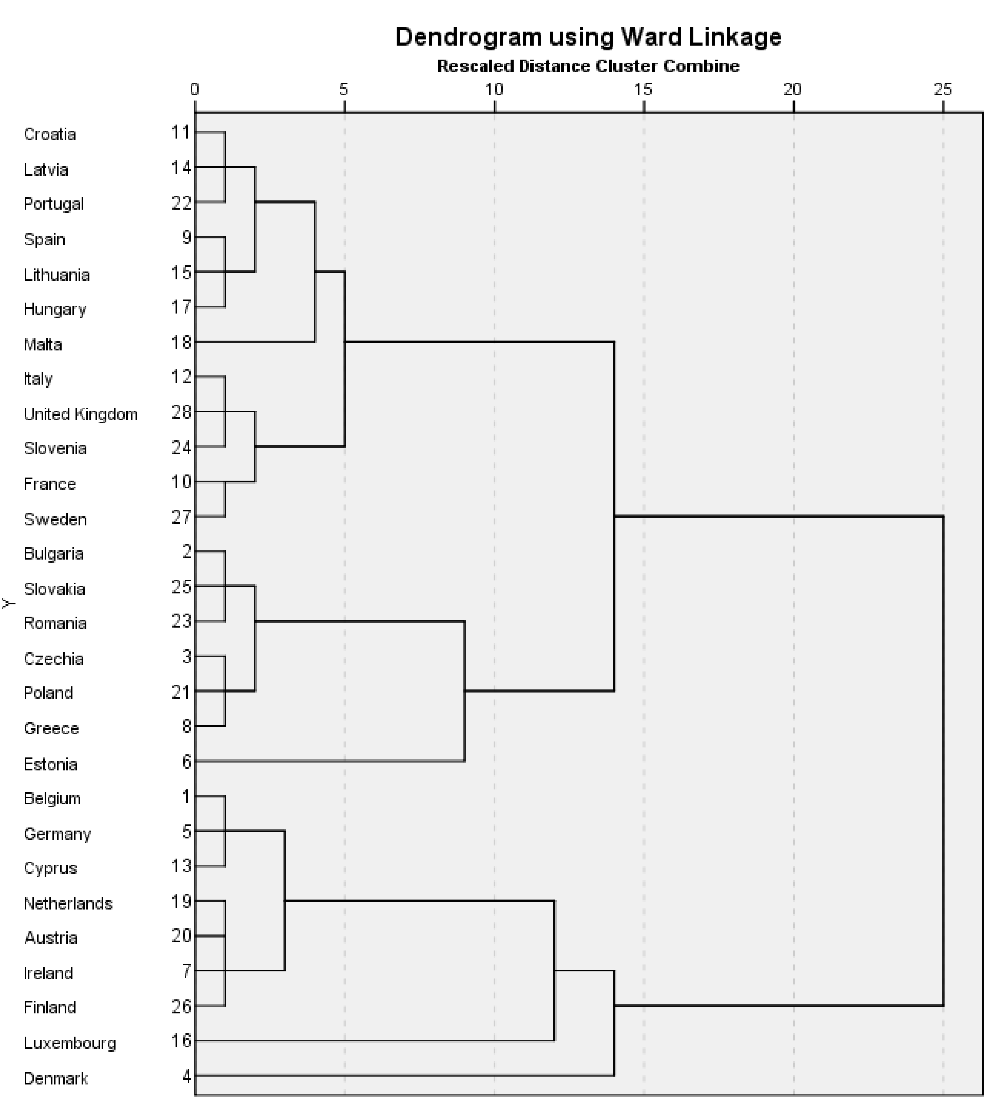
Figure 1 presents the results of non-spatial cluster analysis for the year 2008, the dendrogram using Ward linkage. It shows detected similarities between countries. Based on the dendrogram, we can distinguish the following clusters:

• cluster 1, represented by low GDP and low environmental taxes revenues—mostly new EU member states (Czechia, Malta, Portugal, Slovenia, Bulgaria, Romania, Lithuania, Poland, Estonia, Slovakia, Croatia, Latvia, Hungary);
• cluster 2, represented by high GDP and high environmental taxes revenues (Denmark, Ireland, Netherlands, Sweden, Austria, Finland, Germany, UK, France, Belgium, Spain, Cyprus, Greece, Italy);
• cluster 3, represented by one country with the highest GDP and energy taxes revenues (Luxembourg).

Figure 2 presents the result of non-spatial cluster analysis for the year 2017, the dendrogram using Ward linkage. We can distinguish the following clusters:

• cluster 1, represented by low CO₂ emissions, middle tax revenues and low EU ETS revenues (Croatia, Latvia, Portugal, Spain, Lithuania, Hungary, Malta);
• cluster 2, represented by low CO₂ emissions, high tax revenues and low EU ETS revenues (Italy, UK, Slovenia, France, Sweden);
• cluster 3, characterized by increased CO₂ emissions, low tax revenues, high EU ETS revenues and low GDP (Bulgaria, Slovakia, Romania, Czechia, Poland, Greece);
• cluster 4, represented by one country with the lowest transport tax revenues, high CO2 emissions and the highest EU ETS revenues (Estonia);
• cluster 5, characterized by increased CO₂ emissions, high transport tax revenues and high energy tax revenues (Belgium, Germany, Cyprus, Netherlands, Austria, Ireland, Finland);
• cluster 6, represented by one country with the highest CO₂ emissions and too high tax revenues (Luxembourg);
• cluster 7, represented by one country with low CO₂ emissions and too high tax revenues (Denmark).

3.2. Spatial Clustering

By using the spatial method of cluster analysis, K-nearest neighbors, the results are similar, and the clusters are only slightly different. It is worth noting that for both spatial cluster analyses (for 2008 and 2017), the target number of clusters was based on the results from non-spatial clustering. It allowed us to provide results comparable within the particular year.

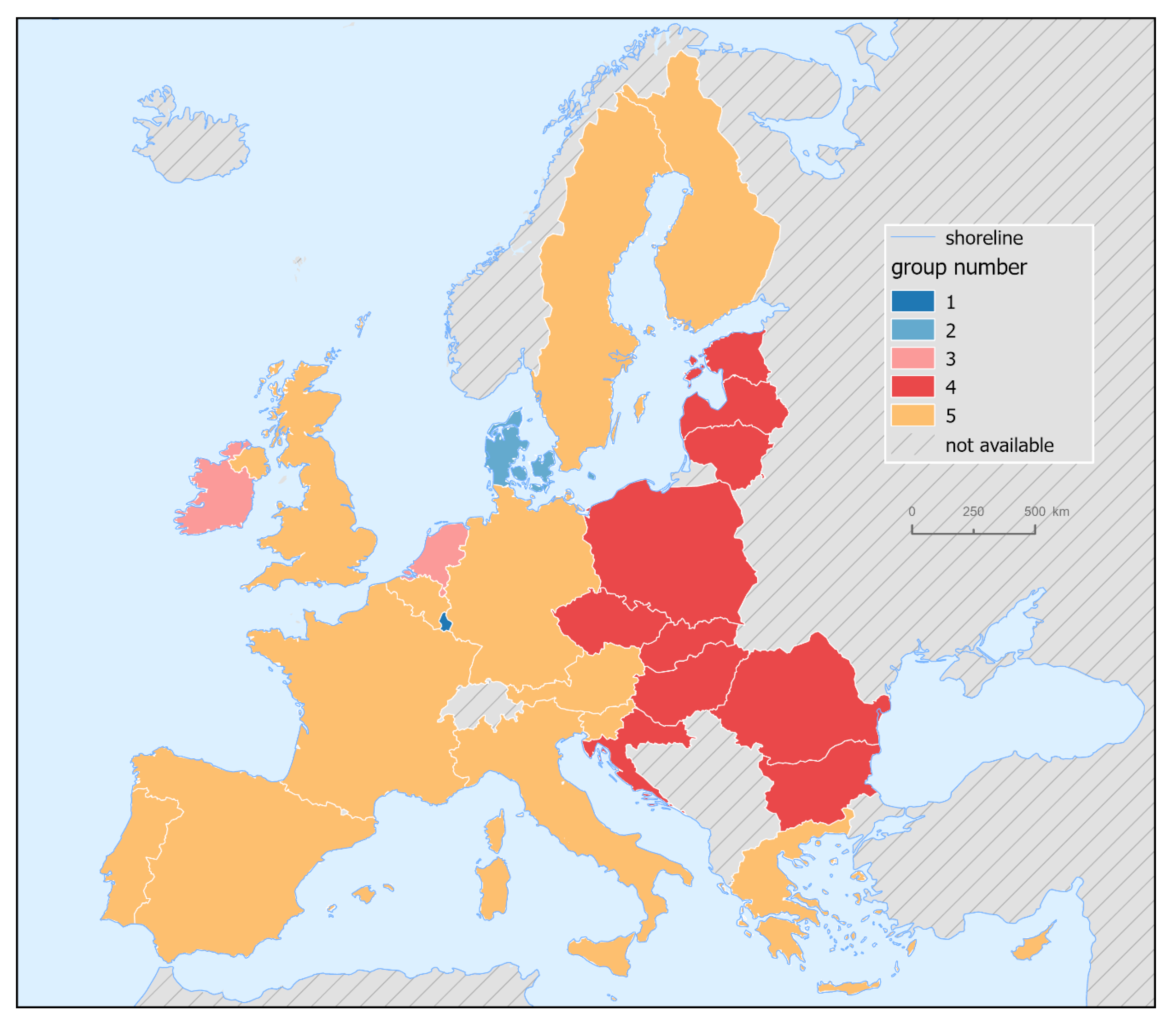
However, as regards the year 2008, when three target clusters (as classified above) was used, the spatial clustering resulted in one cluster containing one country (Luxembourg). This cluster is in line with cluster 3 (using non-spatial clustering). The second cluster consisted of Ireland, Netherlands and Denmark (all in cluster 2 in the non-spatial cluster analysis; together with other countries), and the third cluster contained all 24 remaining countries. Therefore, we decided to test four clusters as a target number (in line with Figure 1 at the level of 2.5 rescaled cluster distance). Again, the result was not satisfactory since the spatial clustering algorithm subtracted only Denmark from the second cluster from the previous step. The “big block” of the remaining 24 countries stayed the same. Consequently, by spatial clustering, we subdivided the “big block” cluster into two separate ones having the final number of five clusters as a result (Figure 3). We decided to keep this division although it is not directly comparable with three clusters from non-spatial clustering.

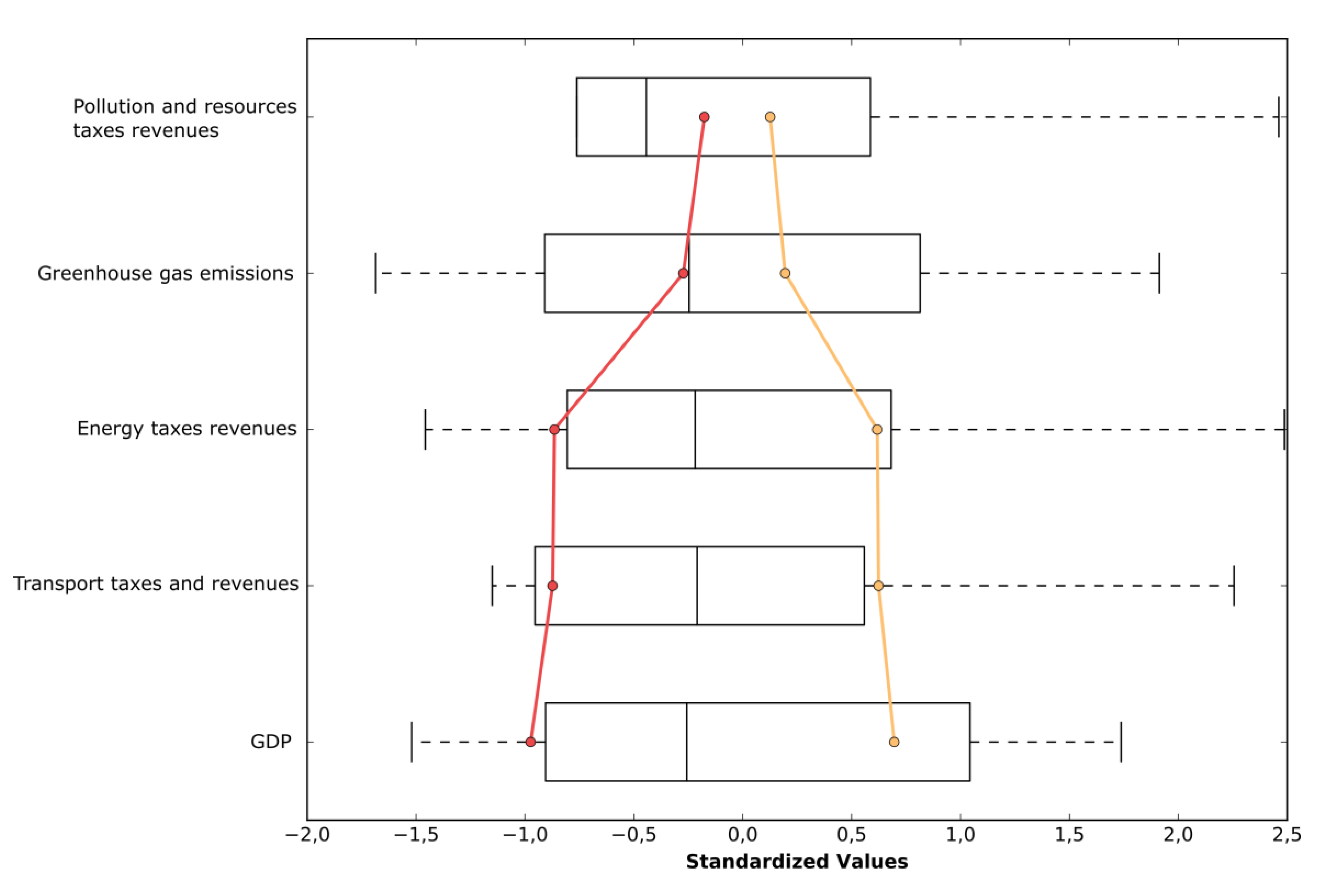
The reason why the Clusters 4 and 5 (former “big block”) were further split in the next step of spatial clustering is evident in Figure 4. The lines follow the opposite trend in energy tax revenues, transport taxes revenues and GDP; almost all of them touching the lower (Cluster 4) or upper (Cluster 5) boundary of IQR (interquartile range). Greenhouse gas emissions are slightly above average in the case of Cluster 5, in case of Cluster 4 around the median. Both clusters evince higher-than-median values in the indicator of pollution and resource taxes. Geographically, both clusters form a majority of “continental” Europe (Great Britain, Norway and Sweden are tight together with “continental” Europe in this case). This result might be explained by mutual geographical proximity and also by the relative similarity of input values. However, it is also evident that Europe is divided into two parts—“east” (Cluster 4) and “west” (Cluster 5)—which might correspond to former geopolitical situations and the history of European countries.

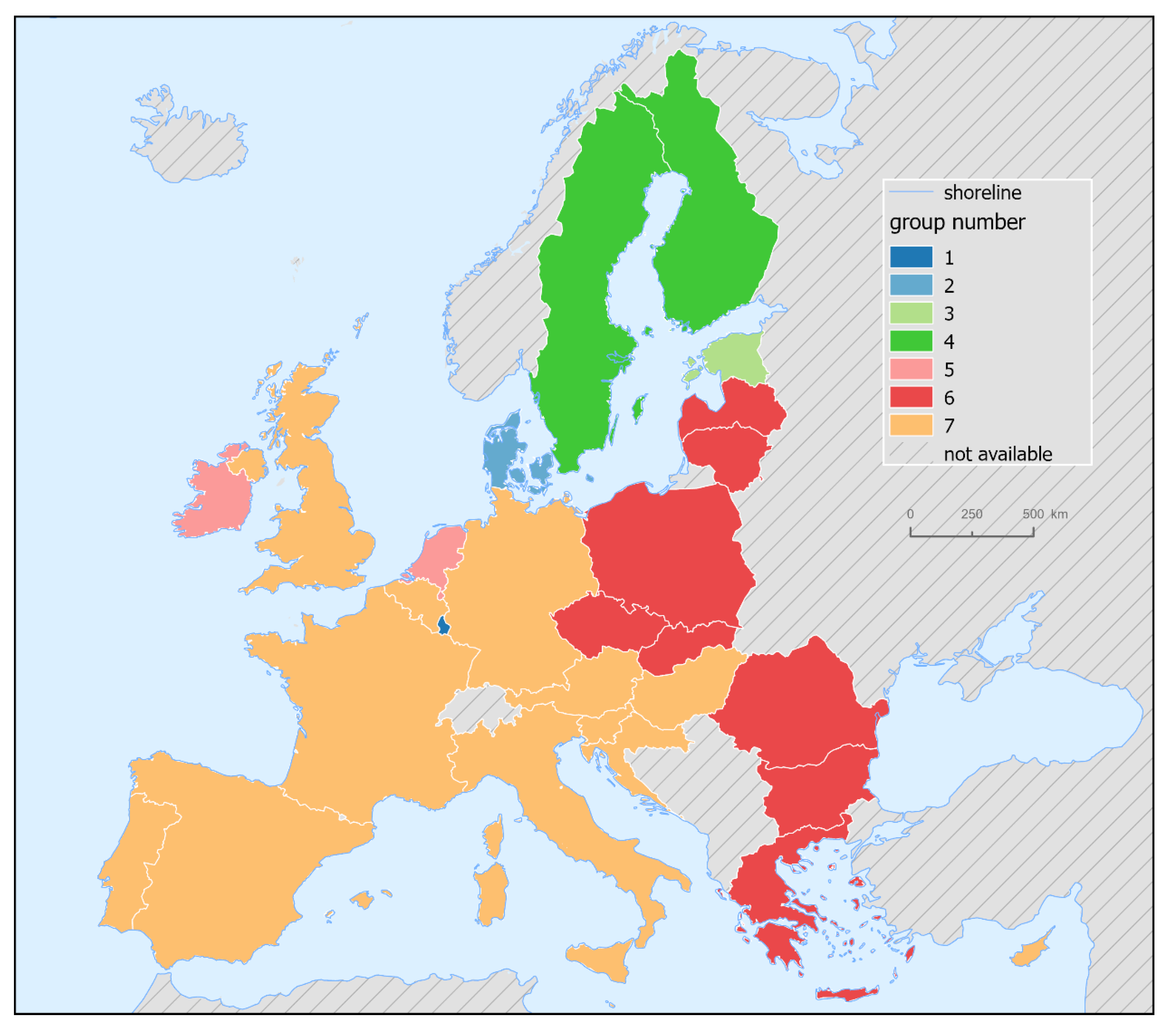
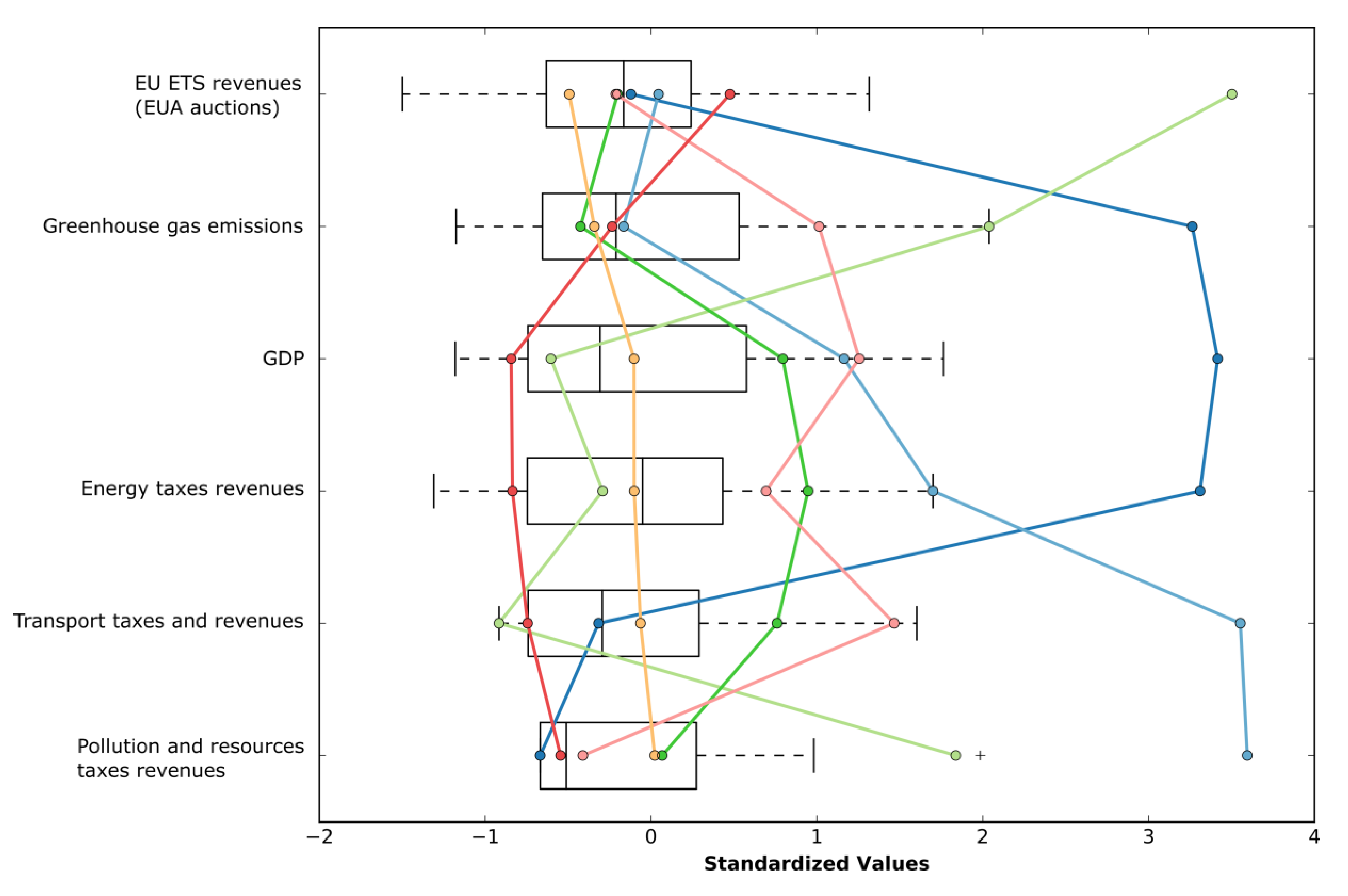
Figure 5 shows the results of spatial cluster analysis for the year 2017. There are three one-member clusters (Luxembourg, Denmark and Estonia); which is in line with findings from non-spatial clustering. Figure 6 shows the parallel box plots as a result of the spatial clustering in 2017. It pinpoints the underlying reasons (from a data perspective) of clustering results and emphasizes individual standardized values of input data.

We can see that the newly formed Cluster 3 (Estonia) expresses extreme values in greenhouse gas emissions, and EU ETS’ revenues (the greatest by far in comparison with other countries/groups). Cluster 1 (Luxembourg) has significantly higher values of greenhouse gas emissions, GDP per capita and energy tax revenues. Similarly, Cluster 2 (Denmark) has extreme values of energy, transport, pollution and resource taxes revenues. Cluster 5 (the Netherlands and Ireland) are typically significantly high (out of IQR) in values of greenhouse gas emissions, GDP per capita, energy and transport taxes revenues, which kept them in a separate cluster. A similar curve trend can be observed in the case of Cluster 4 (Sweden and Finland). The values of input indicators are significantly distinct from Cluster 5, which resulted in the formation of a separate cluster of these Scandinavian countries. Cluster 6 (“east” countries) have all their input indicators’ values (except EU ETS’ revenues) below the average/median. Lastly, Cluster 7 (“west” countries) exposes the input indicators’ values remaining within IQR, moving around the average/median. This cluster could be characterized as “balanced”.

4. Discussion

Based on the results, two interesting observations occur. Firstly, regarding the significance of environmental taxation within the public budgets, EU countries are no longer that strongly divided into the eastern and western parts, as they were in the year 2008. Focusing on the year 2017, we can see a more diverse composition of EU countries in terms of newly formed clusters. Secondly, some countries of Central and Eastern Europe (e.g., Hungary, Slovenia, and Croatia) moved to “western clusters”; Estonia is separated in the new cluster.

Table 5. Common features of clusters in 2008.

Non—Spatial Clusters	Spatial Clusters	Common Features
Czechia, Malta, Portugal, Slovenia, Bulgaria, Romania, Lithuania, Poland, Estonia, Slovakia, Croatia, Latvia, Hungary	Czechia, Malta, Portugal, Slovenia, Bulgaria, Romania, Lithuania, Poland, Estonia, Slovakia, Croatia, Latvia, Hungary	low emissions & low tax revenues
Denmark, Ireland, Netherlands, Sweden, Austria, Finland, Germany, UK, France, Belgium, Spain, Cyprus, Greece, Italy	Sweden, Austria, Finland, Germany, UK, France, Belgium, Spain, Cyprus, Greece, Italy	high emissions & high tax revenues
Luxembourg	Luxembourg	extra high emissions & extra high energy tax revenues & low other revenues
	Denmark	middle emissions & high tax revenues
	Ireland, Netherlands	high emissions & middle tax revenues

Source: own processing.

and

Table 6. Common features of clusters in 2017.

Non—Spatial Clusters	Spatial Clusters	Common Features
Croatia, Hungary, Latvia, Lithuania, Malta, Portugal, Spain	Croatia, Hungary, Malta, Portugal, Spain, Belgium, Germany, Cyprus, Austria, Ireland, Italy, the UK, Slovenia, France	middle emissions & middle revenues
Italy, the UK, Slovenia, France, Sweden	Sweden, Finland	low emissions & high tax revenues
Bulgaria, Slovakia, Romania, Czechia, Poland, Greece	Bulgaria, Slovakia, Romania, Czechia, Poland, Latvia, Lithuania, Greece	middle emissions & extremely low GDP & low tax revenues & high EU ETS revenues
Estonia	Estonia	high emissions & low tax revenues & the highest EU ETS revenues
Belgium, Germany, Cyprus, Netherlands, Austria, Ireland, Finland	Ireland, Netherlands	middle emissions & high tax revenues
Luxembourg	Luxembourg	highest emissions & highest GDP & highest energy tax & low other revenues
Denmark	Denmark	middle emissions & high tax revenues & highest transport and pollution taxes revenues

Source: own processing.

depict and compare the most typical features of individual clusters, both non-spatial and spatial ones, in the year 2008 and the year 2017, respectively. CEE countries are highlighted in both tables.

There are seven distinct groups of countries in the year 2017 (Table 6). Most of the CEE countries are represented predominantly by low tax revenues and high EU ETS revenues, except Croatia, Hungary and Estonia. The deeper observation shows us that in the case of the EU ETS, the revenues from auctions go in parallel with the amount of greenhouse gas emissions. That means the countries with high emissions report high revenues from EU ETS auctions. Concerning taxes, environmental tax revenues are various, regardless of the level of emissions. That means the countries with high emissions can have low, middle and high environmental tax revenues. From the opposite view, the countries with low emissions can have low, middle and high environmental tax revenues, too. It shows us spatial patterns in national priorities and goals connected with environmental taxes and more generally, connected with public budget revenues and economic policy.

Focusing on EU countries, we can find common features of environmental taxation connected with energy taxes and the EU ETS, whereas various EU directives give the rules. On the other hand, in several EU member states national or even local environmental taxes are in force, mainly in the domains of transportation, resources, pollution and products taxation.

Regarding our first research question (“Are there similar characteristics between CEE countries?”), at the beginning of our research we anticipated the answer should be “yes” since a common history and economic structure characterize CEE countries. Based on the results, in the year 2008, the countries were grouped in one cluster, using both methods of cluster analysis. However, in 2017, the situation changed; CEE countries were found to not be grouped only in one cluster, using both methods of cluster analysis. There were several CEE countries in the year 2017 with higher environmental taxation revenues connected with a more active approach to environmental taxes within fiscal policy. This was the case with Slovenia, Croatia, and Hungary. In the case of Hungary, for example, environmental taxes accounted for 2.53% of GDP in 2017 (EU-28 average: 2.4%) and energy taxes for 1.91% of GDP (EU average 1.84%) (Eurostat 2020). The significance of these governmental revenues is revealed by the fact that in the year 2017, environmental tax revenues amounted to 6.6% of total revenues from taxes and social security contributions (EU average 5.97%). Out of this 6.6%, however, the excise tax on the fuel for transport purposes only represented nearly 5%. Following EU emission standards, vehicle registration tax is based on environmental protection considerations, with lower (and sometimes no) rates on hybrid and electric cars. Besides these taxes, pollution-related taxes became more emphatic in the past years in Hungary, including the environmental product fee to cover waste management costs. Lastly, the air, water and soil resource charges were in force throughout the examined period as well (MNB 2019).

As a result of the second research question (“Are there any changes in time, focusing on the years 2008 and 2017?”), we can say that “yes”—there is higher diversification of EU member states in the year 2017.

Concerning the key aspects of fiscal policy, the focus of the policymakers and their policy goals should be defined. As was depicted above, environmental taxes have both fiscal and environmental impacts. The key issue is the major decision of policymakers regarding the level of economic burden connected with environmental protection. Policymakers should generally consider why there are some countries with lower tax revenues than others. As the regional or geographic differentiation also matters, policymakers should take into account local/national characteristics as well. As Jurušs and Brizga (2017) pointed out, politicians rarely take environmental considerations into account, but mostly follow the fiscal aims of the tax and socio-economic arguments trying to balance outside pressure (arising from the European Union environmental policy and acts) and the interests of domestic social partners (business and trade unions). Dealing with EU ETS revenues, some countries are probably better traders and can earn more money from the auctions since the auction prices depend on current demand on the exchange (Pászto and Zimmermannová 2019). According to the significant increase in the price of emission allowances in the period 2018–2020 (from approx. 7 EUR/EUA until approx. 30 EUR/EUA), the influence of revenues from EU ETS auction on state budgets would rise.

Comparing the results with other scientific studies, Liapis et al. (2013) identified that notable groups of countries are Belgium and Italy, Greece and Portugal, Germany and Austria, Finland and Sweden. The other countries are left alone. However, this analysis did not include all EU countries and the environmental tax revenues were not included in the category “tax revenues”. Zaharia et al. (2017) focused on environmental taxation in EU countries, calculated with EU ETS as a part of energy taxes. This study identified the following clusters in the year 2012: cluster 1 comprises Bulgaria, the Czech Republic, Germany, Estonia, Latvia, Luxembourg, Hungary, Poland, Portugal, Sweden, United Kingdom; cluster 2 includes Greece, Italy, Cyprus, Malta, Austria, Finland; cluster 3 consists of Spain, France, Lithuania, Romania, Slovakia; cluster 4 composes of Belgium, Ireland, Iceland and Norway; cluster 5 includes Denmark, Croatia and Netherlands and cluster 6 consists of only one country: Slovenia.

It is important to mention that the cluster analysis is very sensitive to initial settings in both quality and quantity input data (missing values, number of indicators, etc.). Therefore, proper interpretation should be made very carefully.

Regarding the following research, it would be worthwhile to observe yearly changes in clusters in EU countries and the mapping movements of countries between the clusters in more detail. By doing so, we can try to find the groups of countries with the same fiscal policy focus, precisely if their environmental taxes are more transport sector pollution- or energy sector pollution-oriented. It can help focus on changes in policies and trends in the EU as a whole, and in particular countries.

5. Conclusions

The main goal of this paper was to observe possible spatial patterns in fiscal impacts of environmental taxation in EU28, and to depict the groups of countries with the same (or similar) fiscal impact of these instruments on public budget revenues, including environmental and economic characteristics of analyzed countries. For possible spatial pattern identification, the authors used two different methods of cluster analysis, Ward linkage and K-nearest neighbours (spatial) cluster analysis. The analysis was performed for the year 2008 and the year 2017; the year 2008 represents the start of the Kyoto period of the EU ETS; the year 2017 is the last year with all available data and simultaneously can show us the situation after almost decade.

Results show us that in the year 2008, the EU countries were divided into “the west” and “the east”, with some exceptions. The western countries were characterized by high environmental tax revenues, the eastern countries by low revenues. If we focus on the year 2017, the situation is different. The border between old and new EU member states is not so clear. The results show higher diversification between EU countries, concerning the fiscal impacts of environmental taxation. There are seven various groups of countries; low tax revenues and high EU ETS revenues, except for Croatia, Hungary and Estonia, represent most of CEE countries predominantly. The more in-depth observation shows us that in the case of the EU ETS, the revenues from auctions go in parallel with the amount of greenhouse gas emissions. Concerning taxes, environmental tax revenues are various, regardless of the level of emissions. It expresses possible spatial patterns in national priorities and goals connected with various kinds of environmental taxes, and more generally, connected with public budget revenues and economic policy.

This study represents an additional source of information for policymakers, both in CEE countries and the whole EU; it can help them to plan possible changes in environmental taxation, concerning public budget revenues. Moreover, the results of this study fill the gap in the environmental tax analyses field by uncovering spatial patterns of environmental taxation revenues within the EU.

References

- Barrage, Lint. 2020. Optimal Dynamic Carbon Taxes in a Climate–Economy Model with Distortionary Fiscal Policy. The Review of Economic Studies 87: 1–39. [Google Scholar] [CrossRef]
- Bumpus, Adam. G. 2015. Firm responses to a carbon price: corporate decision making under British Columbia’s carbon tax. Climate Policy 15: 475–93. [Google Scholar] [CrossRef]
- EEX. 2020. Emission Spot Primary Market Auction Report 2017. Available online: https://www.eex.com/en/market-data/environmental-markets/eua-primary-auction-spot-download (accessed on 20 April 2020).
- Esri. 2016. How Grouping Analysis Works. Available online: https://desktop.arcgis.com/en/arcmap/10.3/tools/spatial-statistics-toolbox/how-grouping-analysis-works.htm (accessed on 10 September 2020).
- European Commission. 2016. The EU Emissions Trading System (EU ETS). European Union. Available online: https://ec.europa.eu/clima/sites/clima/files/factsheet_ets_en.pdf (accessed on 10 January 2020).
- European Commission. 2019. Evaluation of the Council Directive 2003/96/EC of 27 October 2003 Restructuring the Community Framework for the Taxation of Energy Products and Electricity SWD (2019) 332 Final. Available online: https://ec.europa.eu/transparency/regdoc/rep/10102/2019/EN/SWD-2019-332-F1-EN-MAIN-PART-1.PDF (accessed on 10 January 2020).
- Eurostat. 2013. Environmental Taxes: A Statistical Guide. Available online: https://ec.europa.eu/eurostat/web/products-manuals-and-guidelines/-/KS-GQ-13-005 (accessed on 10 January 2020).
- Eurostat. 2020. Environmental Tax Revenues. Available online: https://appsso.eurostat.ec.europa.eu/nui/show.do?dataset=env_ac_tax&lang=en (accessed on 20 April 2020).
- Everitt, Brian S., Sabine Landau, Morven Leese, and Daniel Stahl. 2011. Cluster Analysis, 5th ed. Hoboken: Wiley. [Google Scholar]
- Frey, Miriam. 2017. Assessing the impact of a carbon tax in Ukraine. Climate Policy 17: 378–96. [Google Scholar] [CrossRef]
- Gemechu, Eskinder Demisse, Isabela Butnar, Maria Llop, and Francesc Castells. 2014. Economic and environmental effects of CO2 taxation: an input-output analysis for Spain. Journal of Environmental Planning and Management 57: 751–68. [Google Scholar] [CrossRef] [Green Version]
- Hair, Joseph, William C. Black, Barry J. Babin, and Rolph E. Anderson. 2010. Multivariate Data Analysis. Upper Saddle River: Prentice Hall. [Google Scholar]
- Hájek, Miroslav, Jarmila Zimmermannová, Karel Helman, and Ladislav Rozenský. 2019. Analysis of carbon tax efficiency in energy industries of selected EU countries. Energy Policy 134: 110955. [Google Scholar] [CrossRef]
- ICE. 2019. EUA UK Auction. Available online: https://www.theice.com/products/18997864/EUA-UK-Auction-Daily-Futures (accessed on 20 April 2020).
- Jurušs, Māris, and Janis Brizga. 2017. Assessment of the environmental tax system in Latvia. NISPAcee Journal of Public Administration and Policy 10: 135–54. [Google Scholar] [CrossRef] [Green Version]
- Labandeira, Xavier, José M. Labeaga, and Xiral López-Otero. 2019. New Green Tax Reforms: Ex-Ante Assessments for Spain. Sustainability 11: 5640. [Google Scholar] [CrossRef] [Green Version]
- Liapis, Konstantinos, Antonis Rovolis, Christos Galanos, and Eleftherio Thalassinos. 2013. The Clusters of Economic Similarities between EU Countries: A View Under Recent Financial and Debt Crisis. European Research Studies 16: 41. [Google Scholar] [CrossRef] [Green Version]
- Lin, Chih-Ming, and Tzai-Hung Wen. 2012. Temporal changes in geographical disparities in alcohol-attributed disease mortality before and after implementation of the alcohol tax policy in Taiwan. BMC Public Health 12: 889. [Google Scholar] [CrossRef] [PubMed] [Green Version]
- Marek, Lukáš, Vít Pászto, and Pavel Tuček. 2015. Using clustering in geosciences: examples and case studies. Paper presented at 15th International Multidisciplinary Scientific Geoconference, Informatics, Geoinformatics and Remote Sensing, Albena, Bulgaria, 18–24 June; vol. 2, pp. 1207–14. [Google Scholar]
- Maršík, Martin, and Daniel Kopta. 2013. Use of the cluster analysis for assessment of economic situation of an enterprise. Acta Universitatis Agriculturae et Silviculturae Mendelianae Brunensis 46: 405–10. [Google Scholar] [CrossRef] [Green Version]
- Magyar Nemzeti Bank (MNB). 2019. Long-Term Sustainable Econo-mix. Budapest: Magyar Nemzeti Bank. [Google Scholar]
- OECD. 2016. Effective Carbon Rates: Pricing CO2 through Taxes and Emissions Trading Systems. Paris: OECD Publishing. [Google Scholar]
- OECD. 2019. Central and Eastern European Countries (CEECs). Available online: https://stats.oecd.org/glossary/detail.asp?ID=303 (accessed on 10 December 2019).
- Pászto, Vít, and Jarmila Zimmermannová. 2019. Relation of economic and environmental indicators to the European Union Emission Trading System: a spatial analysis. GeoScape 13: 1–15. [Google Scholar] [CrossRef] [Green Version]
- Pereira, Alfredo M., and Rui M. Pereira. 2014. Environmental fiscal reform and fiscal consolidation: the quest for the third dividend in Portugal. Public Finance Review 42: 222–53. [Google Scholar] [CrossRef] [Green Version]
- Rozmahel, Petr, Luděk Kouba, Ladislava Grochová, and Nikola Najman. 2013. Integration of Central and Eastern European countries: Increasing EU heterogeneity. WWWforEurope Working Paper, No. 9, WWWforEurope—WelfareWealthWork, Wien. Available online: https://www.econstor.eu/bitstream/10419/125664/1/WWWforEurope_WPS_no009_MS77.pdf (accessed on 10 June 2020).
- Skaličková, Jolana. 2018. Shluková analýza regionů z pohledu lokalizace velkých podniků. Logos Polytechnikos 9: 124–38. [Google Scholar]
- Skovgaard, Jakob, Sofia Sacks Ferrari, and Åsa Knaggård. 2019. Mapping and clustering the adoption of carbon pricing policies: what polities price carbon and why? Climate Policy 19: 1173–85. [Google Scholar] [CrossRef] [Green Version]
- Soetewey, Antoine. 2020. The Complete Guide to Clustering Analysis: k-means and Hierarchical Clustering by Hand and in R. Available online: https://www.statsandr.com/blog/clustering-analysis-k-means-and-hierarchical-clustering-by-hand-and-in-r/ (accessed on 13 November 2020).
- Solaymani, Saeed. 2017. Carbon and energy taxes in a small and open country. Global Journal of Environmental Science and Management 3: 51–62. [Google Scholar]
- Stuhlmacher, Michelle, Sanjay Patnaik, Dmitry Streletskiy, and Kelsey Taylor. 2019. Cap-and-trade and emissions clustering: A spatial-temporal analysis of the European Union Emissions Trading Scheme. Journal of Environmental Management 249: 109352. [Google Scholar] [CrossRef] [PubMed]
- Theodoridis, Sergios, and Konstantinos Koutroumbas. 2006. Pattern Recognition, 3rd ed. Cambridge: Academic Press, 856p. [Google Scholar]
- Van Heerden, Jan, James Blignaut, Heinrich Bohlmann, Anton Cartwright, Nicci Diederichs, and Myles Mander. 2016. The economic and environmental effects of a carbon tax in South Africa: A dynamic CGE modelling approach. South African Journal of Economic and Management Sciences 19: 714–32. [Google Scholar] [CrossRef]
- Ward, Joe. H. 1963. Hierarchical Grouping to Optimize an Objective Function. Journal of the American Statistical Association 58: 236–44. [Google Scholar] [CrossRef]
- Xiangmei, Xue, and Xu Yang. 2018. Temporal and Spatial Distribution Characteristics of Air Pollution Index (API) and its Correlation with the Improvement of Environmental Tax Law. Journal of Environmental Protection and Ecology 19: 471–76. [Google Scholar]
- Zaharia, Marian, Aurelia Pătrașcu, Manuela Rodica Gogonea, Ana Tănăsescu, and Constanta Popescu. 2017. A Cluster Design on the Influence of Energy Taxation in Shaping the New EU-28. Economic Paradigm. Energies 10: 257. [Google Scholar] [CrossRef] [Green Version]
Figure 1.
Results of non-spatial cluster analysis for EU countries in the year 2008—Ward linkage.
Figure 2.
Results of non-spatial cluster analysis for EU countries in the year 2017—Ward linkage.
Figure 3.
Results of spatial cluster analysis for EU countries in the year 2008 (K-nearest neighbors).
Figure 4.
Parallel box plots for cluster 4 and 5, the year 2008.
Figure 5.
Results of spatial cluster analysis for EU countries in the year 2017 (K-nearest neighbours).
Figure 6.
Parallel box plots for four target clusters, the year 2017.