
Multi-Class Assessment Based on Random Forests


Université Côte d’Azur, CNRS, I3S, CEDEX 2, 06103 Nice, France
*
Author to whom correspondence should be addressed.
Educ. Sci. 2021, 11(3), 92; https://0-doi-org.brum.beds.ac.uk/10.3390/educsci11030092
Submission received: 14 January 2021
/
Revised: 9 February 2021
/
Accepted: 18 February 2021
/
Published: 26 February 2021
(This article belongs to the Special Issue Assessment and Evaluation in Higher Education)
Abstract
:Today, many students are moving towards higher education courses that do not suit them and end up failing. The purpose of this study is to help provide counselors with better knowledge so that they can offer future students courses corresponding to their profile. The second objective is to allow the teaching staff to propose training courses adapted to students by anticipating their possible difficulties. This is possible thanks to a machine learning algorithm called Random Forest, allowing for the classification of the students depending on their results. We had to process data, generate models using our algorithm, and cross the results obtained to have a better final prediction. We tested our method on different use cases, from two classes to five classes. These sets of classes represent the different intervals with an average ranging from 0 to 20. Thus, an accuracy of 75% was achieved with a set of five classes and up to 85% for sets of two and three classes.
1. Introduction
Many universities face the same problem: the first-year failure rate is far too high. For example, the average failure rate observed in the first year in France is more than 60%. This is a problem common to all areas, albeit to varying degrees [1]. It is particularly high in France in science, psychology, law, and so on. This phenomenon concerns both small and very large cohorts [2,3]. This failure rate is found both in training courses that do not select their students and in so-called selective training. Faced with this recurring problem, universities are struggling to find a valid explanation as the origins of students is varied. In fact, the studies taken before entering the University are often different from one student to another, the institutions of origin are often of very heterogeneous levels, the students have followed optional courses which vary from others, etc. All these points make it difficult at first glance to identify student profiles that may fail. This is where techniques based on machine learning can be of great help.
The field of educational data mining (EDM) is facing this kind of problem. More precisely, supervised learning techniques have been used more and more in recent years in very different fields, and each time they provide significant support. For example, they are used for image recognition, activity recognition, text classification, the medical field, and emotions. The idea of our project is to use the power of these algorithms to detect the profiles of students entering university who are likely to fail. The algorithms will use learning methods based on the profiles of students from previous years and their success or failure at university. Once such students are identified, it is then possible to set up an adapted pedagogy (tutoring, adapted course, hours of support, etc.) in order to break the spiral of failure. Thus, instead of waiting for students to fail, it will then be possible to set up processes to limit the number of failures.
In this article, we propose a new approach to learn the profiles of failed students. In the following we will present the existing work in terms of prediction of success and profiles, we will present the data from which we work as well as the pre-treatments that we apply to them (in particular in terms of anonymization), we will present then our approach based on Random Forests and we will end with the presentation of our experiments and the promising results that we obtained.
For several years now, research around the world has been interested in this problem of too high failure rates, especially during the first year of university. The vast majority of approaches used are based on supervised learning techniques, but some innovate by testing semi-supervised approaches. In [4], for example, the authors decided to test semi-supervised approaches in order to learn the profiles of failed students. They use an algorithm called the Tri-Learning algorithm. This algorithm is particularly used in cases where it is difficult to label the data [5]. Three classifiers from the original set example are set. These classifiers are then refined using unlabeled examples in the tri-training process.
In his thesis [6], Pojon focuses on the comparison of three significant algorithms of supervised learning to know how much they improve prediction performance. The algorithms he chose are linear regression, decision trees, and Naive Bayes. These algorithms were tested on two datasets, and the decision trees and Naive Bayes gave the best performances.
In [7], the authors compare five algorithms. Faced with the large number of features that make up their dataset, they use feature selection algorithms to reduce it. Among the algorithms used are decision trees and Bayesian networks, Multi-Layer Perceptron (part of the Artificial Neural Network), Sequential Minimal Optimisation (part of the SVM class), and 1-NN (1-Nearest Neighborhood). In this study, the dataset used concerns students admitted to Computer Science in some undergraduate colleges in Kolkata from 2006 to 2012. The years 2006 to 2010 are used to create the model (309 students) and the years 2011 and 2012 are used to test it (104 students). In this study, decision trees gave the best results.
As we have just seen, the studies seem to focus on the same algorithms: the SVM, the Naïve Bayes, the decision trees, as well as the logistic regression [1,4,5,6,8]. The study of existing works has led, on many occasions, to note the points which make this task difficult [8]. These difficulties are intrinsically linked to the nature of the data to be considered. Indeed, these are generally few (it is not uncommon to have to consider student promotions of the order of several tens). These small samples correlate with a large number of characteristics, which can penalize the performances of certain algorithms. Another point that can greatly reduce the performance of predictions is the fact that the datasets considered are generally poorly balanced. It is only very recently that some studies are interested in Random Forests (RF) to solve this problem [2,8,9,10].
The RF algorithm consists of building a set of decision trees (Figure 1). The final decision is taken following a majority vote. The construction of these decision trees is based on two very important concepts: Bagging and Random Feature Selection. Bagging consists of not considering the entire dataset when creating one of the trees of the forest but a subset of randomly selected elements. The Random Selection Feature is a process that occurs at the time of the creation of the nodes of a tree: unlike a conventional decision tree where the creation of a new node is done by choosing the best argument among the set possible arguments, the choice of an argument for the creation of a new node in a forest is done by choosing the best argument among a subset of randomly chosen arguments.
One of the very important results in [11] is the theoretical proof of convergence of RF. That is, the generalization error of RF converges to a limit value with the increase of the number of trees. As demonstrated by Breiman, an upper bound for the generalization error (denoted PE in the original paper) is given by:
where is the mean value of the correlation between two RF models and is the strength of the set of classifiers (i.e., decision trees). As stated by Breiman [11], although the bound is likely to be loose, it fulfills the same suggestive function for RF as Vapnik-Chervonekis-type bounds do for other types of classifiers. It shows that the two ingredients involved in the generalization error for RF are the strength of the individual classifiers in the forest and the correlation between them. The s2 ratio is the correlation divided by the square of the strength. In understanding the functioning of RF, this ratio will be a helpful guide–the smaller it is the better, which means that the error of generalization of the forest will be smaller if the decision from each individual tree is both more reliable and less correlated to the decisions from the other trees.
We have already been able to test the effectiveness of this algorithm in very different domains: the recognition of human activity from videos from a Kinect [12] or worn sensors [13], the classification of short texts [14], the prediction of marine currents, etc. We thus decided to apply this algorithm to try to find relevant answers to the problem of improving student success in their studies.
With this statement, we will show the interest in this technique to answer our problem in this article. We are also aware that the nature of the data we consider requires us to make a significant effort of pre-processing. This is because the dataset contains almost empty columns because all the subjects existing in the school are represented and not all the pupils follow them. Moreover, only the grades obtained in the subjects by the students, the best and worst averages, and the class average are available. A lot of information must be removed from the initial dataset in order to ensure strict anonymization (surname, first name, date of birth, address, telephone, e-mail, etc.). It is also important to be able to obtain indications such as the evolution of grades in a subject over time in order to have a better profile. In the following, we will show the strategies we have implemented to improve our prediction.
2. Material and Methods
2.1. Methodology
We started our research work on a promotion of students which well-illustrated our problem of failure: the first year of studies in computer science of the IUT (Technical University Institute) of Université Côte d’Azur. Indeed, this training is in great demand (more than 2000 requests for 80 to 90 places) and moreover, a selection of the best candidates is made each year. This selection is made by looking at scores in mathematics, French, and English, and also by looking at behavioral remarks. Despite this strict selection process, the failure rate in the first year is still far too high (around 30% in the first year). This type of training is therefore very symptomatic of our problem. We, therefore, worked our study from the list of students admitted in this formation for the school years 2017–2018 and 2018–2019. Over these two years, we have combined, for each student, all the information available concerning their past education with the marks obtained in the first semester of our reference training.
There were many data on past education. They contained the specialties followed by the students, the marks obtained in each subject by the candidate themself and also the average of the class, as well as the highest and lowest averages of the class. We also had information that characterized the high schools of the candidates (number of students having passed the bac, number of honors, etc.). We had thus obtained a fairly large set of data if we considered the information that characterized each candidate for our training. Thus, our initial data set contained more than 400 characteristics. After removing characteristics that were either unnecessary or related to the identity of the students and adding additional information, the dataset contained more than 1000 characteristics. On the other hand, the volume of candidates cumulated over the two years taken into account was around 150, which was obviously not much. Techniques associated with the processing of small data sets should therefore be used in the context of this study [15].
2.2. Data Processing
We first had to encode the data used by the RF algorithm [16]. Some information contained in the dataset can negatively impact predictions, for example, features that mainly have no values. The dataset had been designed to be compatible with all the university’s courses, whatever their field of study. Thus, we considered all the subjects that can be followed before arriving at the university. Our dataset, therefore, contained all existing subjects. However, a high school student cannot follow all these subjects. For example, a high school student who had specialized in a literary field will not have any marks in the final year before university in science subjects such as mathematics or physics and chemistry. Thus, when we consider for our study a university department of studies specializing in computer science, all the columns in our dataset that correspond to non-scientific subjects (literature, Greek, Latin, etc.) will therefore be almost empty.
Thus, we decided not to consider those data. Finally, we added some new data correlated with our dataset. As an example, information about the school of the future students was initially the name of this school and its localization. We replace that information—which was useless—with numerical information related to the number of high school students who obtain their bac, as well as the number of honors.
Finally, we had in our dataset many grades obtained by high school students during their schooling. We calculated other information from those grades, such as the evolution of their results in mathematics during the year, the difference between their best and worst results in a semester, etc. More precisely, we calculated information for each of the subjects followed by the candidates:
- Averages: calculation of averages in all subjects for each term of each school year two by two (première and terminale).
- Weighted averages: weighted averages taking the subjects’ scientific and non-scientific matters. A higher coefficient is given depending on whether the calculated average corresponds to a scientific or non-scientific subject.
- Candidate average delta: candidate average—class average.
- Low average delta: candidate average—lowest average.
- High average delta: highest average—candidate average.
- Difference: difference between the highest and the lowest mark in each subject.
- Range: highest average—lowest average.
- Bonus: (candidate average—average of the class)/(highest average—lowest average).
It emerged that the characteristics that have the greatest influence on prediction obviously depend on one training course to another. Nevertheless, low and high delta values stood out as important characteristics in several formations, so they seemed to be relevant metrics. As seen in article [17], the selection of features improved prediction rates, and the method which gives the best results was the “wrapper” technique [18]. Finally, in order to select a feature on the columns, we chose the “wrapper” technique.
2.3. Class Balancing
The pupil averages to be expected were separated into different intervals called classes. We separated the pupils by their final results. We decided to test different configurations in order to see which one was the most significant. The class numbered 0 was also the most obvious: success, ie [10, 20] in Table 1 means that students obtained an average between 10 and 20, and failure, ie [0, 10[ in Table 1 means that students obtained an average between 0 and 10 (10 is excluded in this range). We also tried to be more precise in our classification. For class number 1, we, therefore, considered pupils with great difficulties (result below 7.5), those who succeed (result above 10), and pupils who have results below 10 but who have not completely failed. As this study was exploratory, we have divided this class into two other similar classes (classes 2 and 3) by slightly modifying the boundaries of each group, as shown in Table 1. Finally, we also planned to separate the pupils into two other even more precise configurations (classes 4 and 5) by dividing the notes into 4 and then 5 intervals.
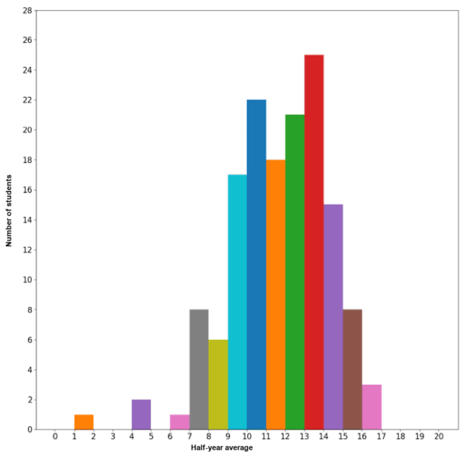
The students were not equally distributed in all the classes, as the majority of them had global results between 9 and 14, as shown in Figure 2. Thus, the number of classes and the limits of those classes had a direct incidence on the number of students in each class.
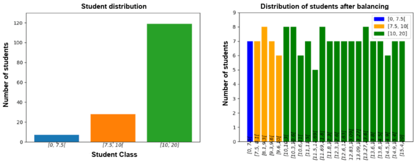
An imbalance in the distribution of students according to class sets was notable. As shown in the following histogram on the left, the class of the pupils having average in range [10, 20] contained 119 pupils out of a total of 154, which represents 77% of the total population. One of the first treatments we had to do on our dataset was to do class balancing in order to minimize this problem.
Class balancing was done in two ways. First of all, the classes with a large population have been divided into subclasses as shown in Figure 3. The disadvantage here is that for some groups, the class population has become small, less than 10 students by class.
The second way was to manage this in the RF algorithm itself, which allows the data of a class with a small population to have greater weight in decision-making. It can be therefore useful to add the hyperparameter “class_weight = balanced”. This automatically weighed classes inversely proportional to the frequency of their appearance in the data.
2.4. Generation of Models
To build the different RF models, we first separate the dataset into two subsets: training dataset, which will be used to build the model, and test dataset, which will be used to test the efficiency of the model. To build the training dataset, we randomly selected 80% of the initial dataset, and the remaining 20% was affected by the test dataset.
As shown in Figure 4, the training dataset was used to build 6 RF corresponding to our six sets of classes, hence creating six models. We then tested those models with the test dataset.
Since the number of students was limited to 154, the test dataset consists of 31 students. This means that each student had a very important weight for the accuracy of the model. Making a mistake on a single student immediately dropped the precision. To face this problem, using several “seeds” made it possible to generate models whose supplied data and definition classes were identical in order to be able to combine their results. The number of seeds used was 150. Thus, the precision was then no longer calculated on 31 pupils but on 4650. This reduces the individual impact of 90% of a prediction and thus had a result closer to reality, to which more confidence can be allowed. In addition, the choice to use 150 “seeds” was taken in order to have results in a reasonable time while having a sufficiently large sample. So, for each set of classes, 150 “seeds” were used.
2.5. Crossover of Models
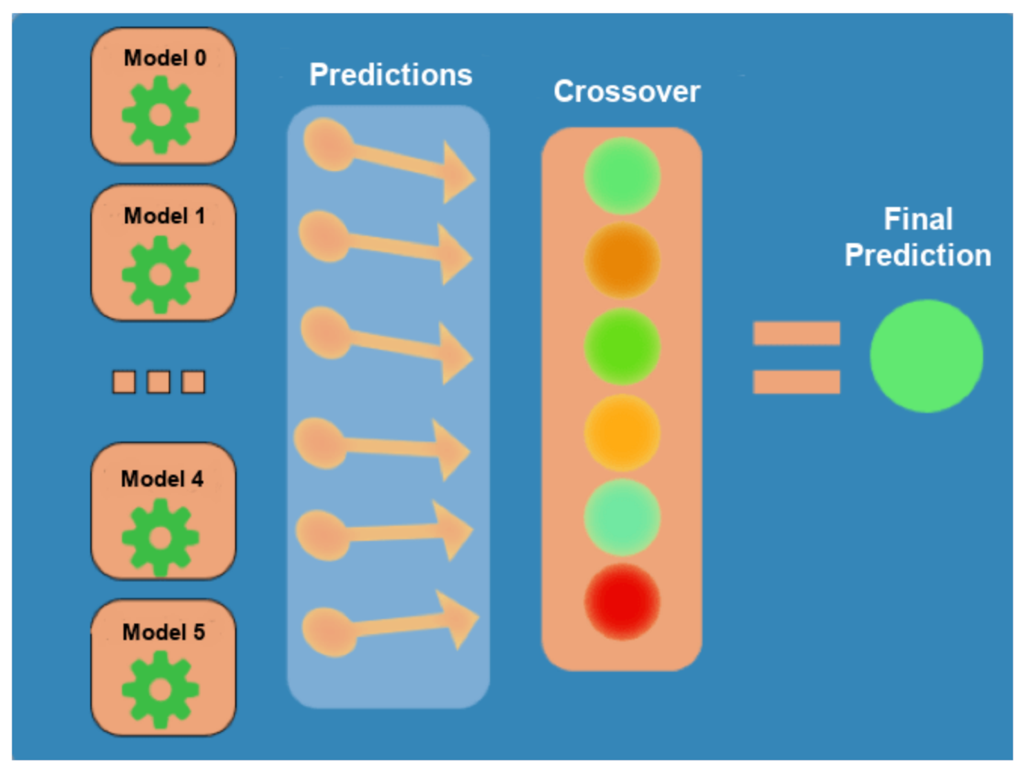
The objective of cross-checking the models was to use the results of the six models trained with the same training set and with different target class sets so that they correct their errors with each other (Figure 5). The goal was to merge their prediction on the same student to try to determine which predictions were wrong.
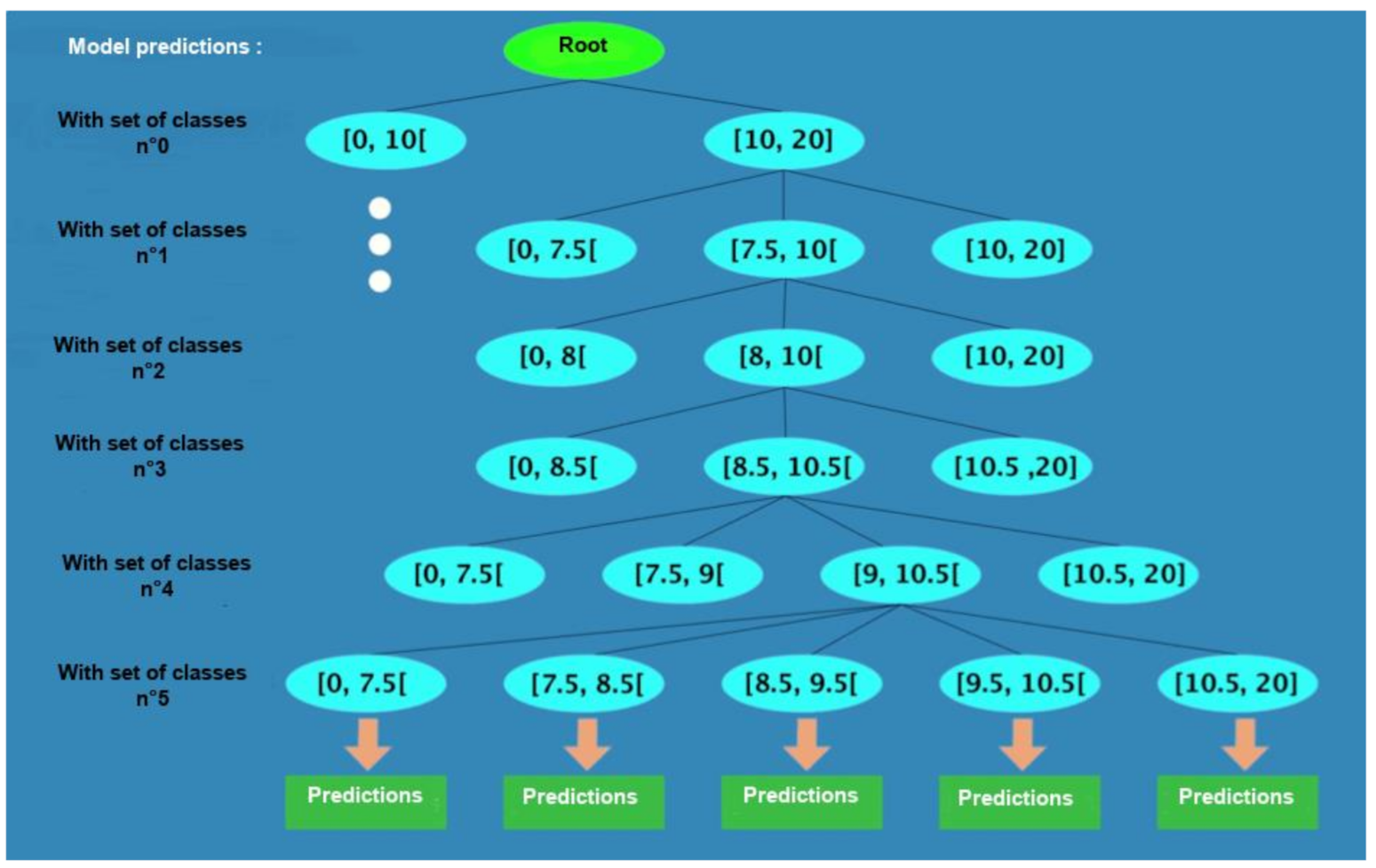
The crossing of the predictions of the six models can be represented as shown in Figure 6. It represents a tree where the last level contains 1081 sheets, where each final leaf represents a possible combination of the predictions of the six models (2 * 3 * 3 * 3 * 4 * 5) for each set of target classes. Each level of the tree represents a model. Each node has m children and m represents the number of classes of the following model. As shown in Figure 6, the class bubble in range [10, 20] of the class 0 set is connected to three child nodes because the class 1 set is made up of three classes. Finally, a tree is made for each set of definition classes.
To know which class to predict after each combination, a training phase was carried out beforehand by making predictions using the models on the students of the test sets. Students whose actual class was different may refer to the same combination of predictions. If so, the class with the highest proportion of students for that combination becomes the combination prediction.
With this process, some combinations may never be encountered. If applicable, the prediction of the model whose definition classes are the same as that of the tree becomes the prediction of the combination of models. For example, if for a combination ‘abcdef’ whose target classes are in range [0, 10[ with 10 cases encountered and range [10, 20] with 30 cases encountered then for this combination the final decision will be a success: the prediction associated with this sheet will therefore be in range [10, 20].
3. Results
Following the increase in data, the balancing of classes, and the crossing of models; the results obtained are shown in Table 2. The “Virtual” column represents the results of the models with the balancing of the classes performed by cutting them up and the “Balanced” column represents the results of the models with the balancing classes performed by weighting the data in the algorithm.
Crossing the models allowed a clear improvement of the predictions, in particular for the models with a larger number of classes such as the models with four and five classes which gained approximately 15% accuracy. After crossing only, the results seem similar with a slight advantage for the models with the “Virtual” class sets. The detailed results after crossing are presented in the form of a confusion matrix (Figure 7) with the prediction of the model on the x-axis and the student’s real class on the y-axis. The diagonal therefore represents the good predictions. First, the results of the models with “Virtual” class sets.
For the classes of students who fail multiclass models, the worst precision is that of class in range [9.5, 10.5[ of model 5 with 27% and the best is that of class in range [7.5, 10[ of model 1 with 57%. Overall, the accuracy for classes of students who fail is about 40% and always over 92% for students who pass. Next, the results of the models with sets of “Balanced” classes (Figure 8).
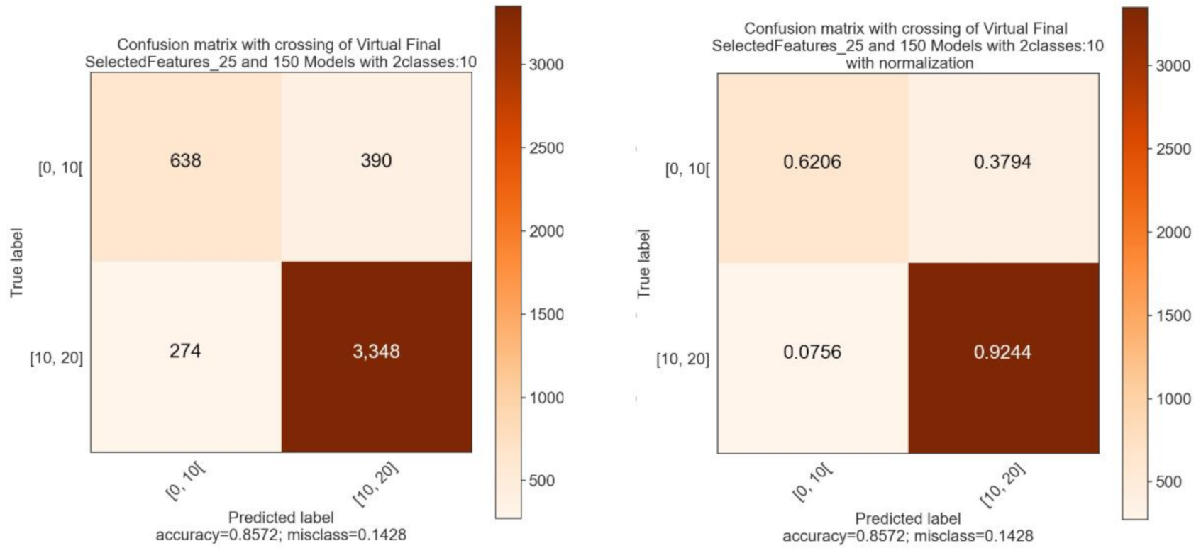
For the two-class model, we observe good precision for the pupils of class in range [10, 20]—more than 95% (Figure 9). However, only 52% of the pupils of class in range [0, 10[ were correctly predicted, which is worse than the model with the previous balancing.
For the classes of students who fail multiclass models, the worst precision is that of class in range [9.5, 10.5[ of model 5 with 17% and the best being that of class in range [7.5, 8.5[ of the same model with 56% (Figure 9). Overall, the accuracy for classes of students who fail is around 40%.
4. Discussion
The confusion matrices show that increasing the number of classes results in a slight loss of precision. The decrease in precision between models with the sets of classes 0,1,2 and 3,4,5 can be explained by the fact that using class [10, 20] offers better precision compared to a model using the class in range [10.5, 20] (Figure 10).
The quality of the prediction of the classes of students who fail is still poor—less than one pupil in two belonging to these classes is correctly identified.
The balancing which seems the most convincing is balancing with the weight of the data because even if there is low precision for the classes contiguous to the classes in ranges [10, 20] and [10.5, 20], the precision of the classes to students with the lowest averages is better. This model is therefore more useful for predicting students who will largely fail than those with an average of around 10/20. The first results were not conclusive. However, thanks to improvements in the data, the increase in features followed by a selection of these led to a gain in model accuracy.
Secondly, balancing the classes of the models allowed for smoothing the precision. That is to say, a gain of precision on the classes with a small amount of data representing them.
Finally, the intersection of the model predictions made it possible to obtain more satisfactory results. However, they are still insufficient because the quality of the prediction of pupils having difficulty is not important enough. However, the models can still be improved.
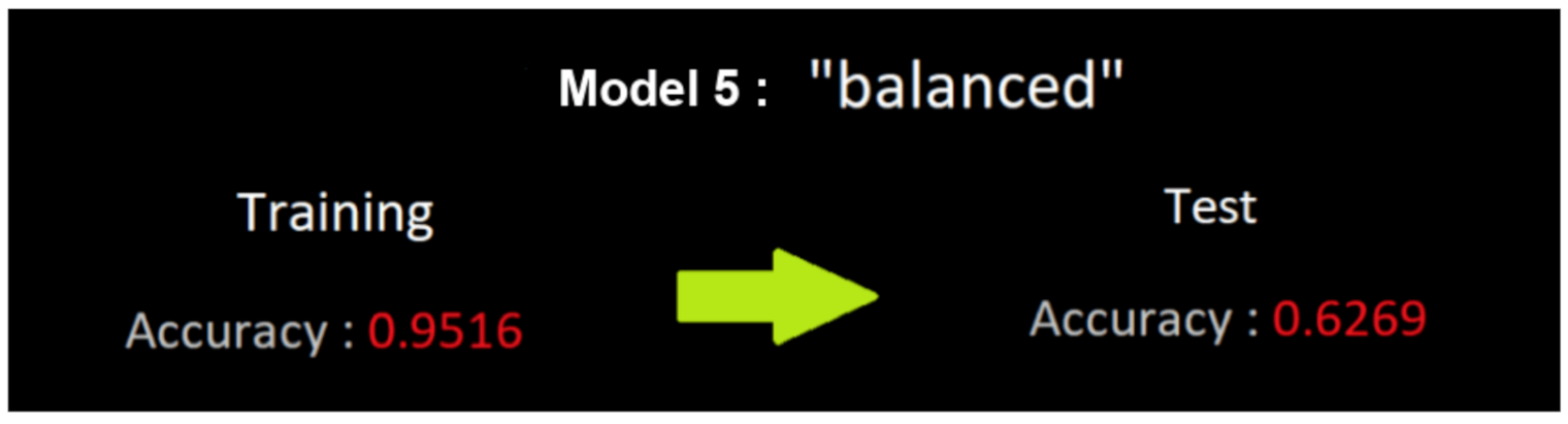
In order to improve the results, we can imagine a second level of crossing predictions between the two kinds of balancing. Improving the RF algorithm, we use is also possible, for example, trying to limit the training so as not to be overfitting as suggested in Figure 11.
5. Conclusions
In this article, we addressed the problem of success in the first year of university by constructing a solution to estimate whether a candidate entering a training course will succeed or not. This additional information can then be used by guidance counselors to guide the future student in their choices and by pedagogical teams to set up specific support measures for each candidate, even before the first evaluations. In order to obtain this information, we used a set of real data that we had previously cleaned and then processed using the RF algorithm. To improve the results, we also implemented a “model crossing” mechanism.
In addition, it should not be forgotten that the results are based on data from first-year students at a Technical University Institute in Computer Science. These have been pre-selected and the size of each promotion can be considered as average, around one hundred. Therefore, wanting to reproduce the process presented to other training is quite possible and relevant. However, the results will probably not be the same since the number of students differs according to the type of training. This can be considered very important like biology or medical training where it can exceed a thousand each year, or low like graphic design schools, for example, Itecom Art Design with around twenty a year. With enrollment differences, the pre-selection of students, as well as the different modules from one training to another, can have an impact on the results.
We are currently working on different solutions to consolidate and improve the results obtained. In addition to the evaluation of different data sources (promotions), we are investigating the possibility of using other algorithms instead of RF and even combining the different algorithms. Finally, we are also starting work to take into consideration not only numerical data characterizing the candidates but also textual data found in class reports.
Author Contributions
Conceptualization: G.R. and C.D.-P.; methodology: G.R. and C.D.-P.; software: M.B. and S.D.; supervision, G.R. and C.D.-P.; project administration, C.D.-P.; All authors have read and agreed to the published version of the manuscript.
Funding
This research received no external funding.
Institutional Review Board Statement
The study was conducted according to the guidelines of the Declaration of Helsinki, and approved by the Institut Universitaire Technologique of Université Côte d’Azur.
Informed Consent Statement
The patient’s consent was revoked because all names and identifying information were removed by persons outside the project. The people who worked on the data were therefore never aware of the source of the data.
Data Availability Statement
Not applicable.
Conflicts of Interest
The authors declare no conflict of interest.
References
- Hussain, M.; Zhu, W.; Zhang, W.; Abidi, S.M.R.; Ali, S. Using machine learning to predict student difficulties from learning session data. Artif. Intell. Rev. 2018, 52, 381–407. [Google Scholar] [CrossRef]
- Wakelam, E.; Jefferies, A.; Davey, N.; Sun, Y. The potential for student performance prediction in small cohorts with minimal available attributes. Br. J. Educ. Technol. 2020, 51, 347–370. [Google Scholar] [CrossRef] [Green Version]
- Hasan, R.; Palaniappan, S.; Raziff, A.R.A.; Mahmood, S.; Sarker, K.U. Student Academic Performance Prediction by using Decision Tree Algorithm. In Proceedings of the 4th International Conference on Computer and Information Sciences (ICCOINS), Kuala Lumpur, Malaysia, 13–14 August 2018; pp. 1–5. [Google Scholar]
- Kostopoulos, G.; Kotsiantis, S.B.; Pintelas, P.E. Estimating student dropout in distance higher education using semi-supervised techniques. In Proceedings of the 19th Panhellenic Conference on Informatics, Athens, Greece, 1–3 October 2015; pp. 38–43. [Google Scholar]
- Zhou, Z.-H.; Li, M. Tri-training: Exploiting unlabeled data using three classifiers. IEEE Trans. Knowl. Data Eng. 2005, 17, 1529–1541. [Google Scholar] [CrossRef] [Green Version]
- Pojon, M. Using Machine Learning to Predict Student Performance. Master’s Thesis, Faculty of Natural Sciences, University of Tampere, Tampere, Finland, June 2017. [Google Scholar]
- Acharya, A.; Sinha, D. Early Prediction of Students Performance using Machine Learning Techniques. Int. J. Comput. Appl. 2014, 107, 37–43. [Google Scholar] [CrossRef]
- Imran, M.; Latif, S.; Mehmood, D.; Shah, M.S. Student Academic Performance Prediction using Supervised Learning Techniques. Int. J. Emerg. Technol. Learn. 2019, 14, 92–104. [Google Scholar] [CrossRef] [Green Version]
- Sultana, J.; Usha Rani, M.; Farquad, H. Student’s Performance Prediction using Deep Learning and Data Mining Methods. Int. J. Recent Technol. Eng. 2019, 8, 1S4. [Google Scholar]
- Shetty, I.D.; Shetty, D.; Roundhal, S. Student Performance Prediction. Int. J. Comput. Appl. Technol. Res. 2019, 8, 157–160. [Google Scholar] [CrossRef]
- Breiman, L. Random forests. Mach. Learn. 2001, 45, 5–32. [Google Scholar] [CrossRef] [Green Version]
- Halim, A.A.; Dartigues-Pallez, C.; Precioso, F.; Riveill, M.; Benslimane, A.; Ghoneim, S.A. Human action recognition based on 3d skeleton part-based pose estimation and temporal multi-resolution analysis. In Proceedings of the IEEE International Conference on Image Processing (ICIP 2016), Phoenix, AZ, USA, 25–28 September 2016; pp. 3041–3045. [Google Scholar]
- Gioanni, L.; Dartigues-Pallez, C.; Lavirotte, S.; Tigli, J.-Y. Using random forest for opportunistic human activity recognition: A complete study on opportunity dataset. In Proceedings of the 11èmes Journées Francophones Mobilité et Ubiquité (Ubimob 2016), Lorient, France, 5 July 2016. [Google Scholar]
- Bouaziz, A.; da Costa Pereira, C.; Dartigues Pallez, C.; Precioso, F. Interactive generic learning method (IGLM): A new approach to interactive short text classification. In Proceedings of the SAC ’16 31st Annual ACM Symposium on Applied Computing, Pisa, Italy, 4–8 April 2016; pp. 847–852. [Google Scholar]
- Fernandez-Delgado, M.; Cernadas, E.; Barro, S.; Amorim, D. Do we need hundreds of classifiers to solve real world classification problems? J. Mach. Learn. Res. 2014, 15, 3133–3181. [Google Scholar]
- Amine, S.; Dartigues-Pallez, C.; Gaetan, R. Classification Supervisée de Données Pédagogiques pour la Réussite dans L’enseignement Supérieur; Master’s Thesis, hal-02486729; I3S Université Côte d’Azur: Sophia-Antipolis, France, February 2020. [Google Scholar]
- Nguyen, C.; Wang, Y.; Nguyen, H.N. Random forest classifier combined with feature selection for breast cancer diagnosis and prognostic. J. Biomed. Sci. Eng. 2013, 6, 551–560. [Google Scholar] [CrossRef]
- Saeys, Y.; Abeel, T.; Van De Peer, Y. Robust Feature Selection Using Ensemble Feature Selection Techniques. In Machine Learning and Knowledge Discovery in Databases; Lecture Notes in Computer Science; Springer: Berlin/Heidelberg, Germany, 2008; Volume 5212, pp. 313–325. [Google Scholar]
Figure 1.
Principle of Random Forests (RF).

Figure 2.
Histogram of the distribution of pupils according to their average.

Figure 3.
Histograms before and after class balancing.

Figure 4.
Model generation process.

Figure 5.
Models crossover.

Figure 6.
Tree representing the model crossing method.

Figure 7.
Tree “Virtual” confusion matrix model number 1 to 3 after crossing.

Figure 8.
“Balanced” confusion matrix for two classes after crossing.

Figure 9.
“Balanced” confusion matrix for five classes after crossing.

Figure 10.
Results of a model with the class in range [10, 20] and of a model with the class in range [10.5, 20].
Figure 10.
Results of a model with the class in range [10, 20] and of a model with the class in range [10.5, 20].

Figure 11.
Accuracy in training and testing.


Table 1.
Set of classes.
| Class Set Label | Class Intervals | ||||
|---|---|---|---|---|---|
| 0 | [0, 10[ | [10, 20] | |||
| 1 | [0, 7.5[ | [7.5, 10[ | [10, 20] | ||
| 2 | [0, 8[ | [8, 10[ | [10, 20] | ||
| 3 | [0, 8.5[ | [8.5, 10.5[ | [10.5, 20] | ||
| 4 | [0, 7.5[ | [7.5, 9[ | [9, 10.5[ | [10.5, 20] | |
| 5 | [0, 7.5[ | [7.5,8.5[ | [8.5, 9.5[ | [9.5, [ | [10.5, 20] |
Table 2.
Accuracy for two balancings.
| Before Crossing | After Crossing | |||
|---|---|---|---|---|
| Class Set | Virtual | Balanced | Virtual | Balanced |
| 0 | 0.79 | 0.81 | 0.85 | 0.85 |
| 1 | 0.71 | 0.755 | 0.848 | 0.84 |
| 2 | 0.68 | 0.76 | 0.84 | 0.83 |
| 3 | 0.63 | 0.68 | 0.77 | 0.76 |
| 4 | 0.59 | 0.63 | 0.76 | 0.75 |
| 5 | 0.56 | 0.626 | 0.75 | 0.74 |
Publisher’s Note: MDPI stays neutral with regard to jurisdictional claims in published maps and institutional affiliations. |
© 2021 by the authors. Licensee MDPI, Basel, Switzerland. This article is an open access article distributed under the terms and conditions of the Creative Commons Attribution (CC BY) license (http://creativecommons.org/licenses/by/4.0/).
Share and Cite
MDPI and ACS Style
Berriri, M.; Djema, S.; Rey, G.; Dartigues-Pallez, C. Multi-Class Assessment Based on Random Forests. Educ. Sci. 2021, 11, 92. https://0-doi-org.brum.beds.ac.uk/10.3390/educsci11030092
AMA Style
Berriri M, Djema S, Rey G, Dartigues-Pallez C. Multi-Class Assessment Based on Random Forests. Education Sciences. 2021; 11(3):92. https://0-doi-org.brum.beds.ac.uk/10.3390/educsci11030092
Chicago/Turabian StyleBerriri, Mehdi, Sofiane Djema, Gaëtan Rey, and Christel Dartigues-Pallez. 2021. "Multi-Class Assessment Based on Random Forests" Education Sciences 11, no. 3: 92. https://0-doi-org.brum.beds.ac.uk/10.3390/educsci11030092
Note that from the first issue of 2016, this journal uses article numbers instead of page numbers. See further details here.