Highly Accurate Digital Current Controllers for Single-Phase LCL-Filtered Grid-Connected Inverters


1
Department of Control, Automation and Computing Engineering, Federal University of Santa Catarina, Blumenau 89036-256, Brazil
2
School of Electrical Engineering, Pusan National University, Busandaehak-ro 63beon-gil, Geumjeong-gu, Busan 46241, Korea
3
School of Electrical Engineering and Computer Science, National University of Sciences and Technology, Islamabad 44000, Pakistan
4
Electrical Engineering Department, Colorado School of Mines, Golden, CO 80401, USA
*
Authors to whom correspondence should be addressed.
Electricity 2020, 1(1), 12-36; https://0-doi-org.brum.beds.ac.uk/10.3390/electricity1010002
Submission received: 25 June 2020
/
Revised: 22 July 2020
/
Accepted: 29 July 2020
/
Published: 31 July 2020
Abstract
:Photovoltaic (PV) systems are the most promising technology for residential installation as an alternative source of energy. To interface the primary source of PV to the electrical grid, an LCL-filtered inverter is being broadly adopted due to its low volume compared to the L-filtered one and the superior ability to filter high-frequency harmonics. In this context, this paper proposes highly accurate digital current controllers for single-phase LCL-filtered grid-connected inverters. The proposed controllers are: Integral-single-lead, integral double-lead, integral double-lead taking into account the effect of pulse width modulation (PWM) delay and the proportional-resonant (PR). These controllers are different from the traditional Proportional-Integral (PI), Proportional-Derivative (PD), and Proportional-Integral-Derivative (PID). One of the novelties of this paper is the detailed, step-by-step procedure for tuning each parameter of the proposed digital controllers considering the dynamic behavior of the LCL filter. The proposed PR has a different and more straightforward tuning methodology than those procedures commonly found in the literature. Therefore, this paper is an attractive tool for a fast, accurate, and reliable way to tune digital current controllers for a single-phase LCL-filtered grid-connected inverter. The controllers were verified in the digital signal controller (DSC) TMS320F28335 while the power structure runs in a hardware-in-loop (HIL device). Results show the efficacy of the proposed controllers.
1. Introduction
1.1. Background and Literature Review
The high penetration of PV system in residences brought new challenges to the distribution utilities. Several concerns never worried about before are now causing severe problems, obliging utilities to impose restrictions on the customers. One such issue is the injection of high frequencies components generated by the pulse width modulation (PWM) of the electronics’ converters used in PV systems [1,2]. This led industries and academia to develop high-order passive filters. After some decades, the LCL-type become the most dominant output filter of power inverters. Some reasons that made the LCL-type one of the best options are the low-volume compared to L-type and the superior ability to filtering high frequencies components. However, the LCL filter presents a natural resonant frequency, which needs particular attention to prevent high oscillation and instability through it.
At the same time, the development of the current controller for LCL-filter grid-connected inverters took special attention in the scientific community. The design of an accurate current controller is vital for the appropriate operation of the inverter. The controller must follow its reference signal with negligible steady-state error and must be able to reject disturbances that may appear in the systems.
Regarding the power distribution system, the LCL-filter inverter usually can be connected to single- or three-phase systems. For residential installations of PV, the connection to a single- or three-phase distribution system often depends on the rated power of the PV and the availability of such systems. For high power PV systems, the three-phase grid is preferably chosen [3]. Nevertheless, for low power and limited availability, several PV systems with LCL-filtered inverter are connected to single-phase distribution system around the world.
Current controllers for LCL-filtered grid-connected inverter are continually being proposed in the literature [3]. There are a variety of types of controllers like the proportional-integral (PI) [4], PR [5], sliding mode, fuzzy-based [6], model predictive control (MPC) [7,8], and so on. Most of the research covering such controllers is proposed for a three-phase system, admitting that the parameters of the distribution system are known and they do not change along time [9]. In case of real violation of such assumptions, the performance of the controller may be deteriorated. Controllers that can operate under uncertainties in the parameters of the distribution system were proposed in [10,11]. Their proposals are for three-phase systems and do not pay the desired attention to single-phase systems.
Three-phase current controllers are mature and very well spread in the literature. In [12], a controller based on state feedback linearization was proposed. The nonlinear system of the LCL-filtered grid-connected inverter is mapped to a controllable standard type. Then, classical linear system control method is adopted to design the controller. A PR controller with the ability to ride through faults in the grid was proposed in [13]. In [14], a control strategy for LCL-filtered inverters was developed for weak grids. The proposed design method can guarantee the inverter stability and robustness simultaneously without needing any compensation network, additional hardware, or the complicated iterative computations that cannot be avoided for the conventional inverter design method.
Regarding controllers for a single-phase LCL-filtered grid-connected inverter, the most dominant is the PR. A PR controller with disturbance rejection was proposed in [15]. The paper uses some state observers, which may not be highly accurate in case of uncertainties. On the other hand, [16,17] presented an optimized method for design current controllers. One drawback of grey wolf optimizer and the state current observe controller methods is the necessity of a sophisticated algorithm leading to use of a relatively low sampling frequency. The PI controller is sometimes employed in a single-phase system. Even knowing that the PI is unable to follow sinusoidal references without null error, its usage is sometimes justified because the PI is designed to present a low and acceptable steady-state error. The procedure for tuning a PI, in this case, can be found in [4]. In [18] the mathematical model of the grid-connected inverter was investigated. Then, its linearized small-signal state-space model was obtained, and a linear quadratic regulator was achieved by the solution of algebraic Riccati equation while in [19] an adaptive control of LCL-filtered with time-varying parameters using reinforcement learning was proposed.
Attempts to use three-phase control strategies in single-phase are also found in the literature. The idea behind that is to preserve the features and simplicity of three-phase in single-phase systems. In this case, simplified controllers can be adopted to make the output current follow its reference signal with negligible steady-state error. The use of PI is largely used. The books [3,9] describe the procedure for designing single-phase current controllers using three-phase approaches. However, the performance of the controller is very dependent on the Phase-Locked Loop (PLL) performance, and there is an effect of axis coupling. In [20,21], the authors proposed a decoupled technique to the direct-quadrature (dq)-reference frame in a single-phase system. The efficacy of the proposal was demonstrated, but it brings complexity to the control strategy and dependence of other functions.
The dynamic characteristics of the LCL filter in DC-DC or DC-AC converter are the same. The differences fall in the nature of currents and voltages across the LCL and in the manner how the elements are charged and discharged. In DC-DC converters, the current through the inductors is DC, having finite, non-null value and ripple. In this context, the LCL elements are analyzed using concepts of DC circuits. Inductors are charged and discharged with positive current, but interchanging the sign of the derivative of the current.
The LCL of DC-AC converters handles AC current and voltage. In this case, the average value of current and voltage is zero. Therefore, the charge and discharge of the LCL elements happens naturally during the cycles of the AC variables. From the point of view of the current controller, the dynamic characteristic of the LCL must be modeled in order to make the most suited controller. Since the controlled current is AC, the controller needs to have high accuracy.
1.2. Novelties and Goals
All the previously mentioned research has their efficacy and legitimacy. However, new issues can be addressed. The integral single-lead and integral double-lead controllers are familiar topics in the literature. However, these controllers were employed only to DC-DC converters and, in most cases, the approach is in the continuous-time domain. The dynamic behavior of the LCL-filtered inverter is entirely different from the dynamic behavior of DC-DC converters, requiring special care in tuning the controllers. In this context, the use of the controllers mentioned above was not properly investigated in the literature for applications in LCL-filtered grid-connected inverters.
This paper brings to the state of the art about controlling single-phase grid-connected inverters a proper design procedure for tuning the integral single-lead and integral double-lead controllers considering the dynamic behavior of the LCL-filtered inverter. These controllers are different from the traditional PI, PD, and PID. To enhance accuracy, there is also a proposal of a tuning procedure taking into account the PWM delay effect on the integral double-lead controller. Finally, a digital PR controller was also proposed. The proposed PR has a different and simpler tuning methodology then those procedures commonly found in the literature. While conventional procedures for PR controllers in the literature deal with complex and trigonometric equations, the proposed procedure for the PR controller is simpler and straightforward. The step-by-step procedure for computing each parameter of the four proposed digital current controller is carefully presented. The proposed controllers can be applied to LCL-filtered inverters with passive and active resonance damping.
Some advantages of the proposed controllers are: It does not need to know the grid impedance for their designing, there is no need for voltage feedforward action, it does not need variable transformation as found in alpha-beta and dq-reference frames, it works in a satisfactory manner in weak grids and voltage with harmonic distortions, it is not dependent on the performance of a PLL, it takes into account the current sensor gain, it can be used in three-phase abc-reference frame control strategies, and it can be employed for active and passive damping-based LCL filters.
The controllers covered in this paper are defined as highly accurate digital current controllers. The reason for such a definition is because there is an equation for each parameter of the controllers. No one parameter is computed by trial-and-error or empirical methods. Moreover, for digital implementation, the coefficients of the controllers were programmed with 11 decimal places. This results in highly accurate digital controllers.
Therefore, this paper contributes to presenting an attractive guide for a fast, accurate, and reliable procedure for tuning digital current controllers for a single-phase LCL-filtered grid-connected inverter.
2. Single-Phase LCL-Filtered Grid-Connected Inverter
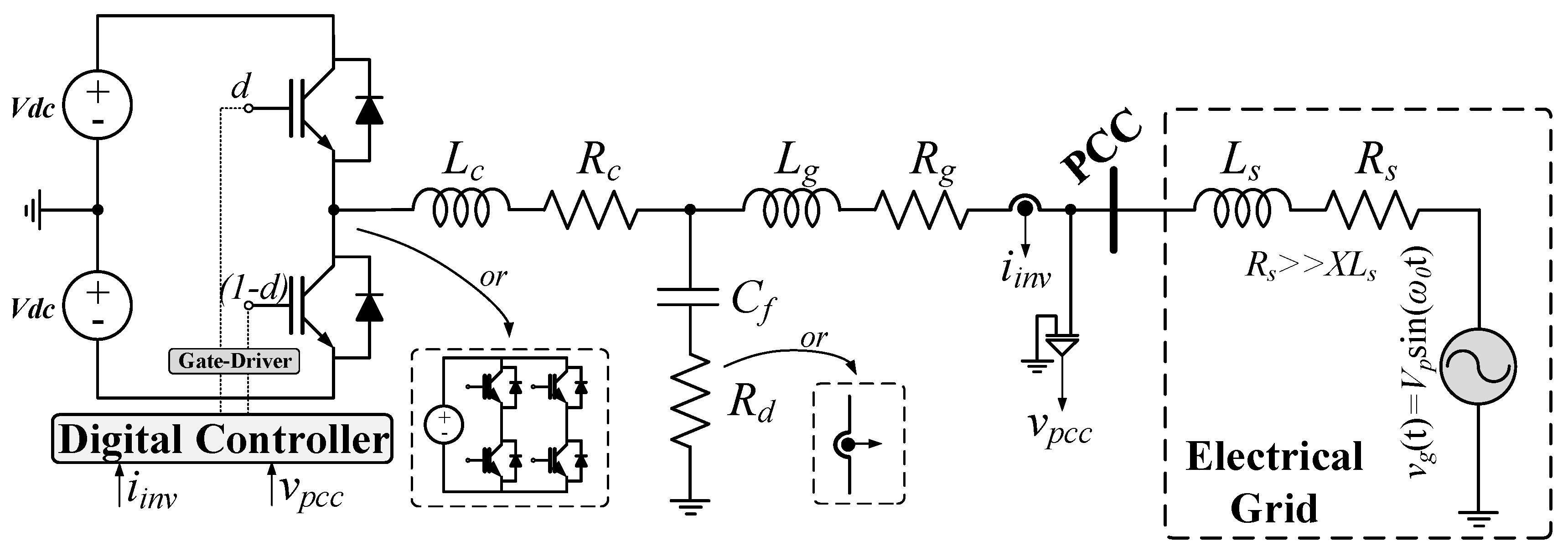
Figure 1 presents the LCL-filtered inverter connected to a single-phase power distribution grid. The inverter is made by a half-bridge converter with two DC sources. Nevertheless, all the content of this paper is also valid for a full-bridge converter with one DC source, as indicated in the figure. The DC sources represent the PV system plus a DC-DC converter. For the sake of verification of the proposed controllers, the DC sources will be assumed with fixed value and also with a fixed-plus-10% of oscillation. The LCL components have the letters c, g, f, and d as subscripts, meaning converter-side, grid-side, filter, and damping, respectively. The LCL has a passive damping action, even though the content of this paper is also valid for active damping action based on capacitor current feedback. The LCL-filtered inverter is connected to the point of common coupling (PCC). The grid-side inductor current and the PCC voltage are measured and sent to the digital control strategy. The PCC voltage is used only to generate a synchronized current reference signal while the grid-side inductor current is used as feedback to the controller. The block of the digital controller is a simplification of the control strategy, having the Analog to Digital Converter (ADC), Zero-Order Holder (ZOH), PWM, and the proposed controllers. The electric grid has a line impedance, represented by and . The relation of is preserved since this is commonly found in residential power distribution grids. The values of them are not necessary for tuning the proposed controllers.
The DC sources in Figure 1 may also represent other sources instead of a PV system with DC-DC converter. They may represent batteries or a DC link of back-to-back converter. For such cases, a bidirectional power flow is usually required. The procedures for tuning the digital current controllers are also valid when there is a need of bidirectional power flow. As will be observed later, the controllers are able to make the output current follow sinusoidal reference with negligible steady-state error. The direction of power, i.e., from the grid or to the grid, is dependent on the phase displacement of the current reference signal with the PCC voltage. For a power flow from the DC sources to the grid, the phase displacement is null. For a power flow from the grid to the DC sources, the phase displacement is 180°. In both cases, the reference is sinusoidal. Therefore, the controllers are able to handle bidirectional power flow.
3. Highly Accurate Digital Current Controllers
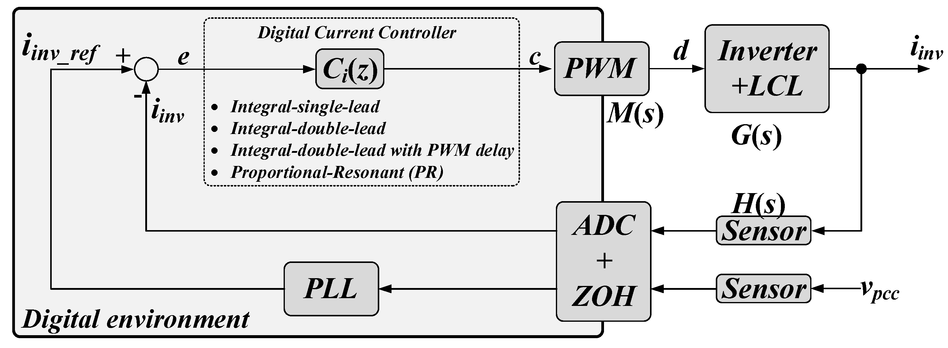
Figure 2 presents a simplified diagram of the control strategy. The larger rectangle shows the digital environment. The inverter output current and the PCC voltage are measured through sensors and sent to the Digital Signal Controller (DSC) via a conditioning circuit (not shown). The DSC has an ADC with a sampler and zero-order holder (ZOH). The PCC voltage passes in a PLL [22,23] to generate a synchronized reference signal. The reference is compared to the inverter output current. The result is the error signal, which in turn is applied to the current controller . The figure shows that the current controller can be one of the highly accurate controllers proposed in this paper. The PWM interfaces the DSC and the LCL-filtered inverter. Note that both the PWM and LCL-filtered inverter are described by transfer functions in s-domain. This is necessary to properly design the digital current, as explained in the following.
The PLL used in the control strategy deservers special attention. Its purpose is only to generate a clean sinusoidal signal, synchronized with the PCC voltage. Such a signal is used as reference to the output current of the LCL-filtered inverter. The performance of the four digital current controllers shown in Figure 2 is independent of the performance of the PLL. Taking as example control strategies running in dq-rotating reference frame [24], if the PLL fails to be accurately synchronized with the PCC voltage, the control strategy will not perform as expected because the reference frame will not be correct. As a result, the inverter output current may present a highly distorted waveform and the whole system may become unstable. In the proposed controllers, if the PLL fails to be accurately synchronized with the PCC voltage, the inverter output current keeps following the reference signal, even though it may exist a short phase displacement between the output current and the PCC voltage. Obviously, this is not a desired situation. To overcome that, the PLL must assure the generation of a clean and synchronized reference signal even under distorted voltage grid.
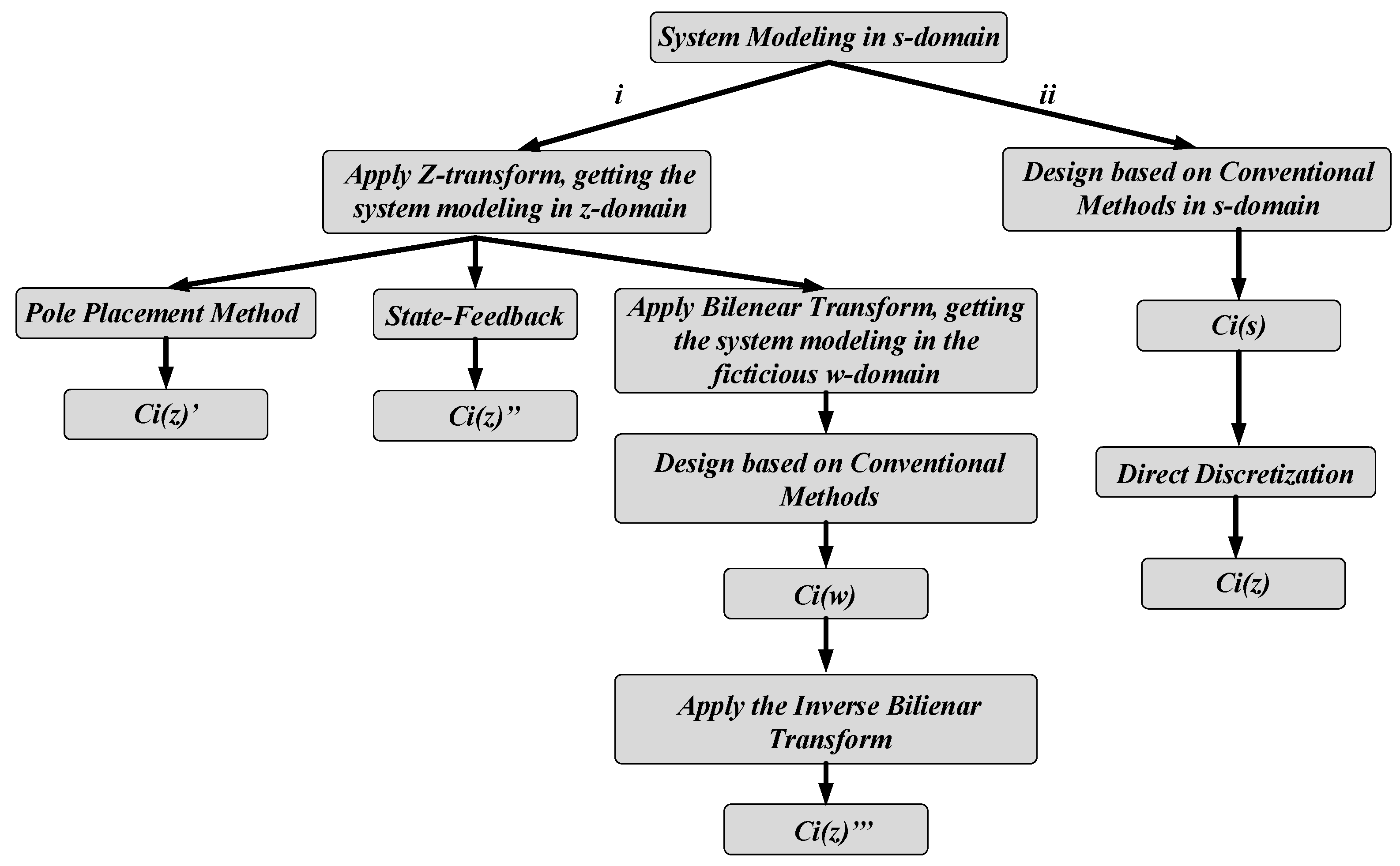
Independently of what kind of controller is employed in the control strategy, tuning the parameters may be performed in a variety of manners. Figure 3 shows a chart of the most traditional methods for tuning a digital controller. Starting from the system modeling in s-domain, the designer can choose between two paths: (i) apply the Z-transform in the s-domain model, getting the z-domain model. In this approach, the effect of the ZOH is taken into account. Then, the current controller can be tuned through pole placement [25], state-feedback [26,27], and through conventional methods using the fictitious w-plane [28]. These methods, even though very mature and broadly adopted, have some drawbacks. The pole placement method is not trivial because the designer must define the location of the poles in the closed-loop system. The state-feedback method requires the measurement of several variables and its performance is deteriorated under parameter variations. The conventional methods through w-plane require several domain transformations, leading to inaccuracy. On the other hand, the designer can choose the path (ii). By choosing that, the controller is designed in s-domain, and later it is discretized, reaching the digital controller. For the majority of applications, this method results in an accurate controller up to the Nyquist frequency. Throughout this paper, path (ii) is adopted. The designed current controllers will be plotted with their equivalent s-domain controllers to show the accuracy of them. Moreover, the choice for path (ii) justifies the definition of the PWM in s-domain as shown in Figure 2.
3.1. System Modeling in s-Domain
The dynamic model of the LCL-filtered grid-connected inverter is commonly found in the literature. Its obtaining procedures as well as the dimensioning of the LCL components are beyond the scope of this paper, but are found in [24,29,30]. The transfer function that relates the grid-side current and the inverter duty-cycle is defined as and given by
where is the inverter gain, defined as:
The previous equations are valid for the LCL filter with passive damping, as shown in Figure 1. For the case where active damping with capacitor current feedback is employed, the transfer function that relates the grid-side current and the inverter duty-cycle is [4]:
where is the coefficient gain of the active damping action. Throughout this paper, Equation (1) is adopted for tuning the proposed, highly accurate digital current controllers. Nevertheless, Equation (3) could be used as well. The elements and were neglected in (2) and (3) because their effects in the dynamic characteristic of the LCL filter are almost null. Their values can be approximated to zero without loss of generalities. Neglecting and is a common practice in LCL applications, as observed in [29,30,31].
The transfer function of the PWM without considering the effect of its delay is given by:
where is the amplitude of the carrier signal. The numeral 2 in the denominator is due to the double-update method used in the PWM [25].
The transfer function of the PWM, taking into account the effect of its delay, is given by the Pade’s approximation as [32]:
Note a minus signal in front of the equation. The variable is the PWM delay, given by:
where is the sampling frequency. In this case, the switching frequency is equal to the sampling frequency. The choice of the sampling frequency must respect the Nyquist criteria in order to avoid the aliasing effect [28] and must be sufficiently high to allow the computation of all required calculus for a proper operation of the control strategy. Assuring that will avoid losing switching periods. Regarding the switching frequency, the choice of its value usually depends on the technologies of the employed semiconductors and on passive components volume requirements. The procedures proposed here are valid for any kind of transistor technologies and for any value of switching frequency.
The value of 1.5 that appears in (6) is due the natural one-sample delay of digital applications summed with half-sample of the computational time needed to run the control strategy. The value of 1.5 is largely adopted in control strategies when the delay is modeled [3]. Other values may be used as 1 or 2, depending on the design specifications. In this paper, the value 1.5 is enough for taking into account all the delays presented in the system.
The current sensor is modeled with a transfer function in s-domain. Its definition is just the sensor gain , given by:
According to Figure 2, the open-loop transfer function (OLTF) without considering the current controller is given by:
The subscript u means uncontrolled. It is essential to highlight that may be replaced by and for depending on the system configuration and the interest in considering the effect of the PWM delay.
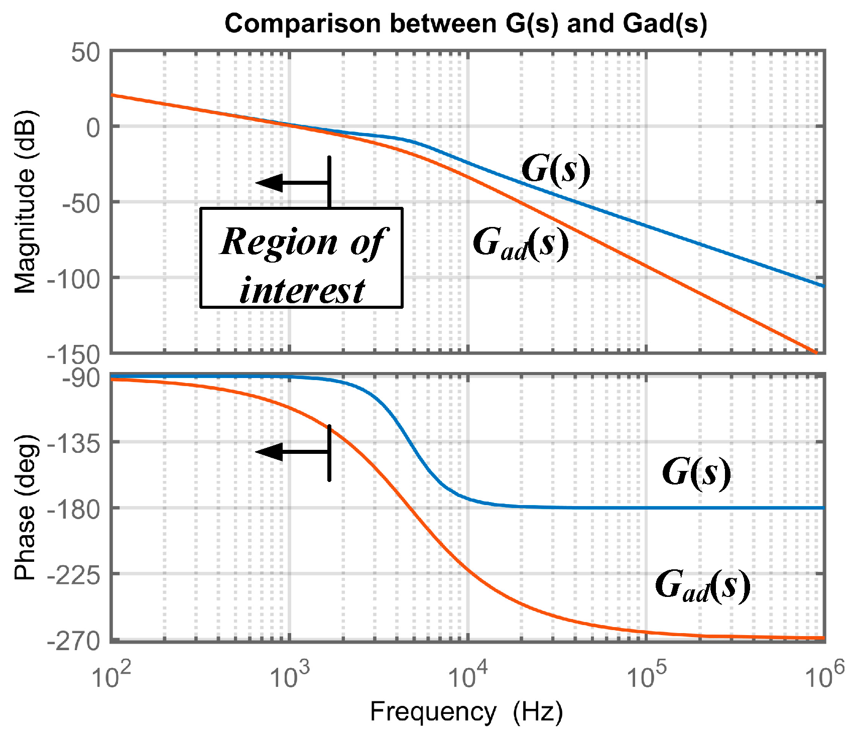
For the sake of comparison, Figure 4 presents the Bode diagrams of the transfer function that relates to the grid-side current and the inverter duty-cycle considering passive and active damping. In this case, the switching frequency is 10 kHz and the value for is 0.55. The figure shows a region of interest, which is from approximately 1.5 kHz and below. Such a region is the region where the controller acts, taking into account that the desired cutoff frequency for the system should be from 8 to 10 times lower than the switching frequency [33]. The curves are almost coincident for the magnitude, while there is a slight difference in the phase curves. This justifies that the proposed controllers presented in the next sections are useful for both methods of LCL damping, the passive and active. Considering the active damping method will require a more significant phase advance in the controller, the proximity of these curves also depends on factor.
The procedures presented in the following sections are independent of each other. Even though they have coefficients named equally, they are not directly related. In other words, the coefficient in the integral single-lead controller is not the same as the coefficient in the integral double-lead controller. This is also valid for all variables that appear in the procedures. The choice of using the name of the same coefficients in different controllers is to keep the method as simple as possible. Additionally, the procedures proposed in this paper may serve as a guide for tuning current controllers. The reader can follow only the procedure of the controller that best fits his or her goals.
3.2. Tuning the Integral Single-Lead Digital Current Controller
The integral single-lead controller has a pole at the origin and a single pole–zero pair. The pole at the origin is an integral part of the controller, while the pole–zero pair is responsible for leading the phase [32]. Throughout this paper, this controller will be called . Its transfer function in s-domain is given by:
The procedure for tuning the integral single-lead controller starts with the definition of the desired cutoff frequency , in Hz, and the desired phase margin , in degree. The most recommended definition of the cutoff frequency is to pick a value that is 8 to 15 times lower than the switching frequency, while the phase margin is any value from 30 to 90°. With that defined, the next step is to get the value of the phase at the desired cutoff frequency in the uncontrolled OLTF. This is expressed as:
Similarly, the value of the gain at the desired cutoff frequency in the uncontrolled OLTF is given by:
The gain at the desired frequency obtained in the previous equation is in dB and must be converted into real value. This is performed by:
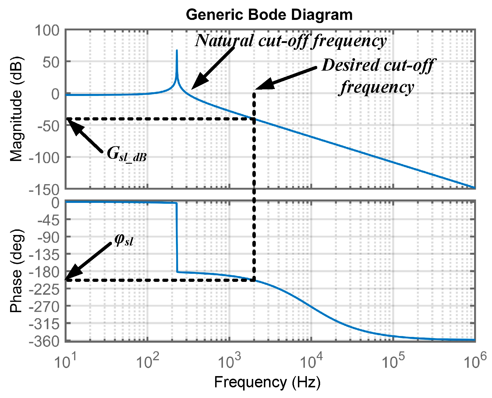
To better visualize where is located in a Bode diagram, Figure 5 shows a generic Bode diagram indicating the points for the desired cutoff frequency, the phase , and gain at the desired cutoff frequency. This Bode diagram is just for illustration and has nothing to do with the system covered in this paper.
The phase that the integral single-lead controller must lead is given by:
The 90° in the equation is due to the phase delay caused by the controller itself [32]. The maximum phase that the integral single-lead controller is able to lead is 90°, as will be shown later. In case there is a need for lead more than 90°, the integral double-lead controller should be used.
At this point, it is convenient to define the following constant:
In this way, the parameters of the current controller in s-domain are given by the following equations:
By computing the four previous equations, the integral single-lead current controller in the s-domain is finally tuned. Before discretizing the controller, it is necessary to check if the desired cutoff frequency and phase margin were obtained. To do that, the OLTF considering the designed controller is given by:
The subscript c means controlled.
The closed-loop transfer function (CLTF) is given by:
Since the cutoff and the phase margin are in accordance with that desired values, the controller is discretized. The integral single-lead current controller is discretized through the backward Euler approximation [28], given by:
where is the sampling period. The result of the previous equation is the digital current controller whose transfer function is given by:
The following equations give the coefficients of the digital current controller:
This ends the tuning procedure for the integral single-lead digital current controller.
3.3. Tuning the Integral Double-Lead Digital Current Controller
The integral double-lead controller has a pole at the origin and two pairs of zero–pole. This controller can lead the phase twice higher than the integral single-lead controller. Throughout this paper, the integral double-lead controller will be called . Its transfer function in s-domain is given by:
The procedure for tuning the integral double-lead controller also starts with the definition of the desired cutoff frequency , in Hz, and the desired phase margin , in degrees. For convenience, the desired cutoff frequency and phase margin will be the same as from the previous. As a result, the names of these variables are preserved.
The next step is to get the value of the phase at the desired cutoff frequency in the uncontrolled OLTF, expressed as:
In a similar way, the value of the gain at the desired cutoff frequency in the uncontrolled OLTF is given by:
The gain at the desired frequency obtained in the previous equation is in dB and must be converted into real value. This is performed by:
Note that the previous three equations are the same for the integral single-lead controller. It is worth highlighting that in case the phase to be led can be obtained by using the integral single-lead controller (lower than 90°), the use of the integral double-lead controller is unnecessary.
The K-factor for the integral double-lead controller is given by:
The value of is the same as previously computed. Notice that the K-factor for this controller is different from the previous one. The parameters of the current controller in s-domain are given by the following equations:
The integral double-lead current controller in the s-domain is finally tuned. The OLTF considering the designed controller is given by:
The closed-loop transfer function (CLTF) is given by:
Since the cutoff and the phase margin are in accordance with the desired values, the controller is discretized. The integral double-lead current controller is also discretized through the backward Euler approximation [28], given by:
The result of the previous equation is the digital current controller whose transfer function is given by:
The coefficients of the digital current controller are given by the following equations, together with the definition of five constants, to :
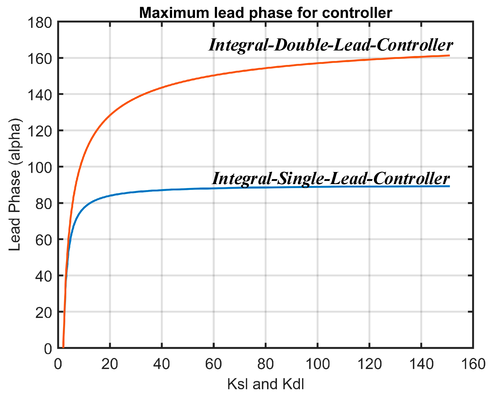
Effectively completing all procedures for the integral double-lead digital current controller, the next section will continue with further recommendations. However, it is necessary to take special view on the lead phase that the integral single-lead and integral double-lead controllers can employ. Figure 6 shows the relation between lead phase versus the K-factor for both controllers. The integral single-lead controller can lead the phase at most 90°, as previously mentioned. As observed, increasing the K-factor from 50 and beyond will not result in an increase in the lead phase. On the other hand, the integral double-lead controller has its maximum lead phase at 180°. This chart is useful because depending on the value the designer computes for in the previous procedures will define what controller can or must be used.
3.4. Tuning the Integral Double-Lead Digital Current Controller Considering the PWM Delay Effect
The two previous controller tuning procedures neglected the effect of the PWM delay. Neglecting such effect is quite acceptable in designing current controllers for LCL-filtered grid-connected inverters, since the switching frequency is usually high and the time constant of the controller is relatively low. However, one may desire to take into account the effect of PWM delay on the procedure for tuning the controller. This section presents the tuning procedure for the integral double-lead digital current controller considering the PWM delay effect. As will be observed later, the consideration of the PWM delay effect does not cause any change in the magnitude curve of the OLTF, but it modifies the phase curve.
In this context, the transfer function of the PWM is presented in Equation (5) and repeated here for simplicity.
The OLTF without considering the current controller is passes to be:
From now on, the procedure for tuning the integral double-lead digital current controller is the same as the previous one and will be omitted here, paying attention that the previous equation takes over.
In the end, the transfer function of the designed controller is given by the following equation, paying attention that the coefficients here are different from the previous ones, even though they are named equally.
For the sake of illustration, Figure 7 presents the OLTF for both considering and not considering the effect of the PWM delay. The magnitude curves are coincident, as expected. The phase curves are slightly different for the region of interest. The controller must lead to a higher phase when taking into account the PWM delay. Such an increase in the value of the phase to be driven is to compensate for the PWM delay.
3.5. Tuning the Digital Proportional-Resonant Controller
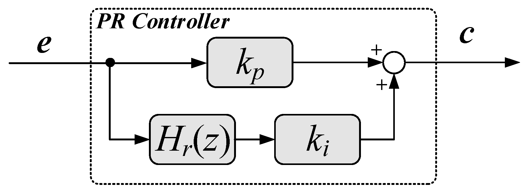
The three previous digital controllers were implemented by a digital filter, defined by a z-domain transfer function. This means that the digital current controller shown in Figure 2 can be one of the following controllers: , , or . The implementation of the digital PR controller is different. Figure 8 show the block diagram of how the digital PR controller is implemented [5]. The PR controller is made by a proportional gain , a resonant gain and a digital resonant filter, which in the z-domain transfer function is named .
The procedure for tuning the digital PR controller consists of obtaining the proportional and resonant gain, as well as the coefficients of the digital resonant filter. The procedure proposed in this paper differs from those commonly found in the literature. There, the proportion and resonant gains are computed using nontrivial trigonometric functions [4]. Here, the procedure is more simplified and accurate.
The first step is to define the desired parameters of the PR controller. They are:
- Desired resonant frequency in Hz and rad/s, named and , respectively. This frequency must be the grid frequency because the PR controller acts in the fundamental frequency for proper active power injection of the LCL-filtered grid-connected inverter.
- Damping factor, named . Any value between 0.9 and 1 is a good choice.
- Desired bandwidth of the resonant filter in Hz and rad/s, named And .
- Sampling frequency in Hertz and period in seconds, named and .
Notice that the current sensor gain is considered in computing the proportional gain. The resonant gain is obtained as:
The next step is to obtain the coefficients of the resonant filter . This is done by applying the Z-transform in its equivalent analog notch filter. The transfer function of an analog notch filter is given by:
Note that the above transfer function is defined in s-domain and it represents a non-ideal notch filter. By applying the Z-transform, it reaches the z-domain transfer function of the digital resonant filter, given by:
The coefficients are given by the following Equations, from (67) to (73).
By computing the previous equations, the tuning procedure for the digital PR controller is finished.
4. Case Study
This section presents a case study of tuning the integral single-lead, integral double-lead, integral double-lead considering the PWM delay effect and PR controllers based on the previous procedures. Table 1 shows the system parameters. The desired cutoff and the desired phase margin are listed at the end of the table.
Applying the values of Table 1 in the four procedures presented in Section 3 result in the designed digital current controller, whose final coefficients are listed in Table 2. The last column listed the coefficients of the digital resonant filter. The proportional and resonant gains are listed at the end of the table.
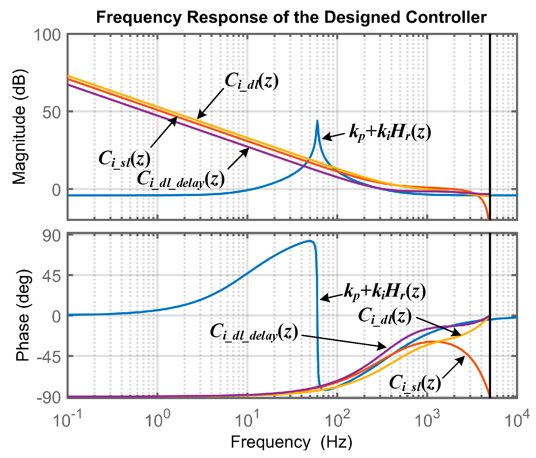
Figure 9 presents the frequency response of the designed digital current controllers. Note that the PR controller is written as , which is the final transfer function of such a controller. At the desired cutoff frequency the controllers have similar behaviors, valid for magnitude and phase curves. This proves that the four covered types of controller are actually enough to control the output current of an LCL-filtered grid-connected inverter. The PR controller has a resonant peak at 60 Hz, showing that its design is accurate.
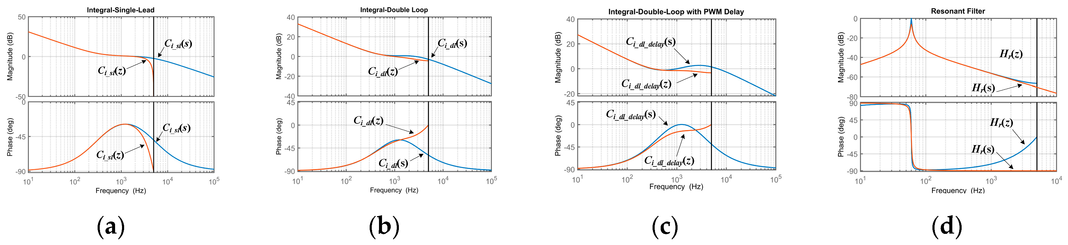
Figure 10 presents the Bode diagrams of the designed current controller in the s-domain and z-domain. For all of them, the curves for magnitude and phase are almost coincident, especially at the desired cutoff frequency. This proves that the methodology of designing a digital controller based on conventional methods in s-domain and later applying a discretization technique is valid and highly accurate. For the PR controller, Figure 10d, only the comparison of the resonant filter is shown for better visualization. Figure 10d also shows that the gain is unitary (0 dB) only at 60 Hz. All other frequencies are attenuated. As a result, only the 60 Hz component will pass through this filter. Another point that deserves attention is that the phase is slightly different in the s and z domain. This means that the obtained phase margin is different from the desired one. However, such difference is minimal and does not invalidate the proposed tuning procedure.
It is important to highlight that in Figure 10 the three first controllers present high gain at 120 Hz. It means that they are able to minimize considerably the effect of the double-frequency pulsation commonly found in single-phase applications. For the PR controller, Figure 10d, and since its approach is to operate at 60 Hz, the ability to minimize such a pulsation is shown as a very low gain at 120 Hz. For the low-frequency region, the three first controllers present high gain. This is attractive because the steady-state error is inversely proportional to the gain at very low frequencies. For the last controller, the analysis of the steady-state error is different. For this case, the error can be computed at the tuned frequency. At the tuned frequency, the gain is 0 dB, which is 1 in real values. This means that the output variable is equal to 1 multiplied by the input. As a result, the output is equal to the input, as expected for component at the tuned frequency.
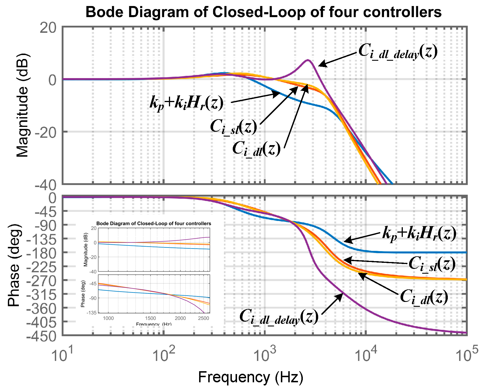
Figure 11 presents the Bode diagram for the closed-loop transfer function considering the designed current controllers. Note that the curves are for the closed-loop transfer function. The names of the controllers pointing at them are just in indication of what controller was used to plot such a curve. These diagrams are plotted in s-domain. Concerning the magnitude curves, the implementation of the proposed controllers makes the closed-loop system present similar behavior along the frequencies in the region of interest. For low frequencies, all of them present a gain of , which makes the steady-state error to be null. At the cutoff frequency, the curves begin to fall. The curve for PR controller begins to fall first because its tuning procedure is different from the other controller regarding the definition of the desired cutoff frequency. In the phase curves, it is evident that all of them are stable and reached the desired phase margin. A zoom is presented for better visualization.
5. Hardware-in-Loop Experimental Verification
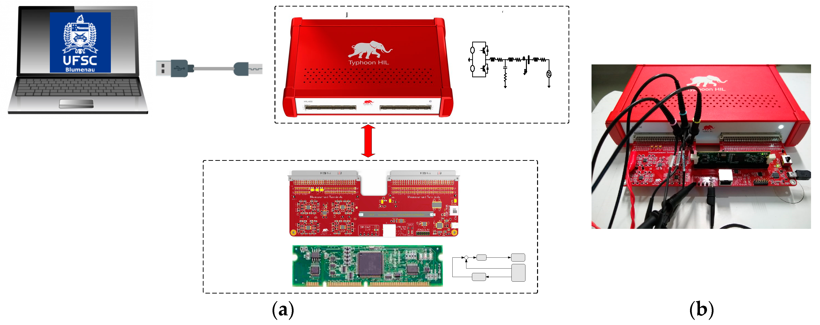
The control strategy presented in Figure 2 was experimentally verified in the DSC TMS320F28335 while the power structure was emulated in the HIL 402 device from Typhoon company. The digital current controller designed in Section 4 was implemented one by one. Results were collected using a desk oscilloscope. Figure 12 presents a diagram of the experimental and HIL verification as well as a picture of it. The HIL sends a signal of variables along the power structure to the DSC through the interface board. In this case, the signals that are sent are the inverter output current and the PCC voltage. The DSC runs the control strategy with the digital current controller and generates the PWM signal, which in turn acts in the HIL. The DSC is connected directly in the interface board. Once the HIL has fidelity to emulate power electronic systems in real time, the DSC receives, processes, and sends signal to the HIL in a similar way of real systems. Therefore, from the point of view of the DSC, the proposed, highly accurate digital current controllers for a LCL-filtered grid-connected inverter is verified experimentally. To visualize in the oscilloscope the reference signal, which is within the DSC, the digital-to-analog converter (DAC) of the interface board was used. The reference signal in the following results show some steps due to the DAC are buffer-type and the relation of the sampling frequency and the reference signal frequency is not an integer number. However, the reference signal within the DSC is purely sinusoidal. This is verified in the inverter output waveforms presenting sinusoidal shape.
The interface board is needed to fit the signals that come from the HIL and go to the analog inputs of the DSC. The HIL delivers signal varying from −5 to 5 V while the DSC supports signals ranging from 0 to 3 V. Therefore, there was a need for programming, such as compensation in the DSC. The amplitude and offset compensation programmed into the DSC was not shown in Figure 2. Another gain adjustment was necessary before the digital current controller as for the integral single-lead, integral double-lead, and integral double-lead with PWM delay effect and as for the PR controller. These amplitude, gain, and offset adjustments are just for implementation purpose and do not invalid the tuning procedures of the current controllers.
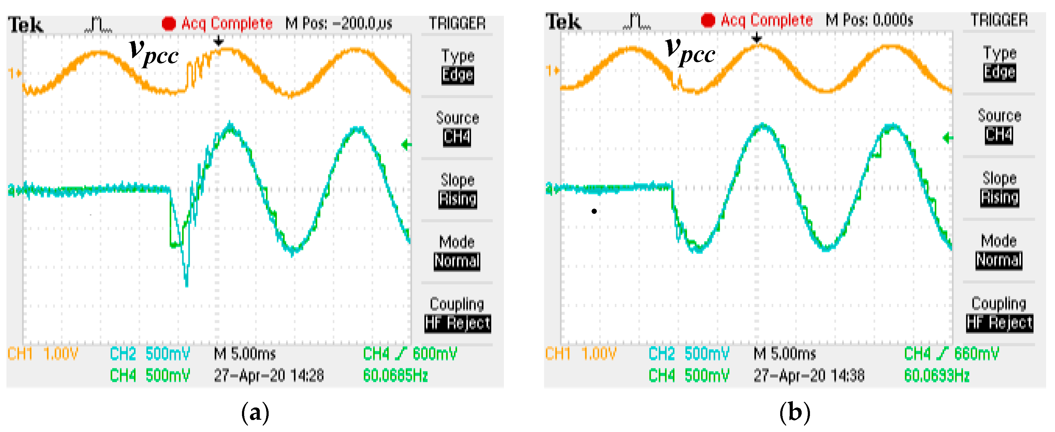
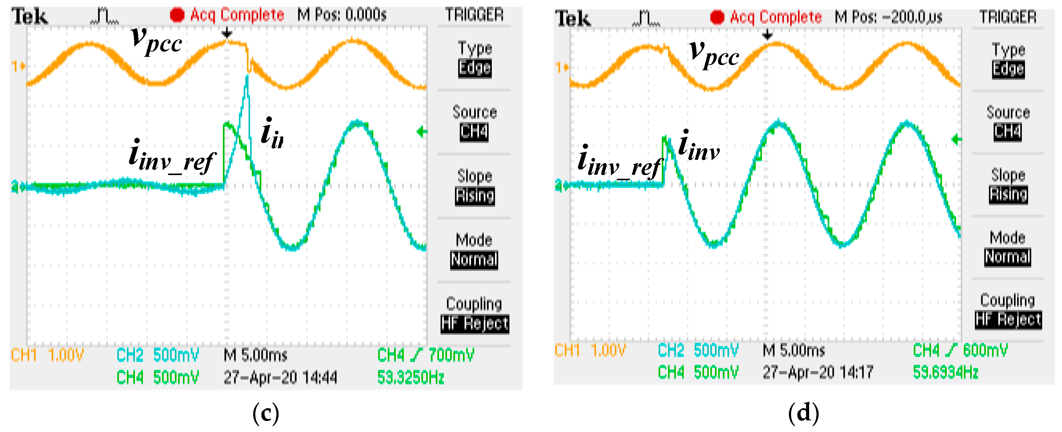
Figure 13 presents the PCC voltage, the inverter output current, and its reference signal for the four designed controllers during initializing. Initially, the reference is null. Later, the reference goes to its maximum value. Before and after the initialization, it is clear that the output current is following its reference with negligible steady-state error for all controllers. This shows the efficacy of the highly accurate, proposed controllers and their tuning procedures. During transitory behavior, the PR controller shows superior performance. Even though the integral single-lead and integral double-lead considering the PWM delay effect showed relative high overshoot, this could be minimized by imposing the reference at zero phase of the grid or making a slow ramp on its amplitude. To show the behavior of the controllers, the time of the reference step was applied randomly. Concerning the PCC voltage, its waveform is not purely sinusoidal, showing a typical power distribution voltage grid with . This is valid for before and after the initialization of the inverter. This is attractive because it shows the ability of the proposed controller to work in weak grids, which are the most severe for current controllers. Another point that deserves attention is that the controller designed without considering the PWM delay effect showed a satisfactory performance.
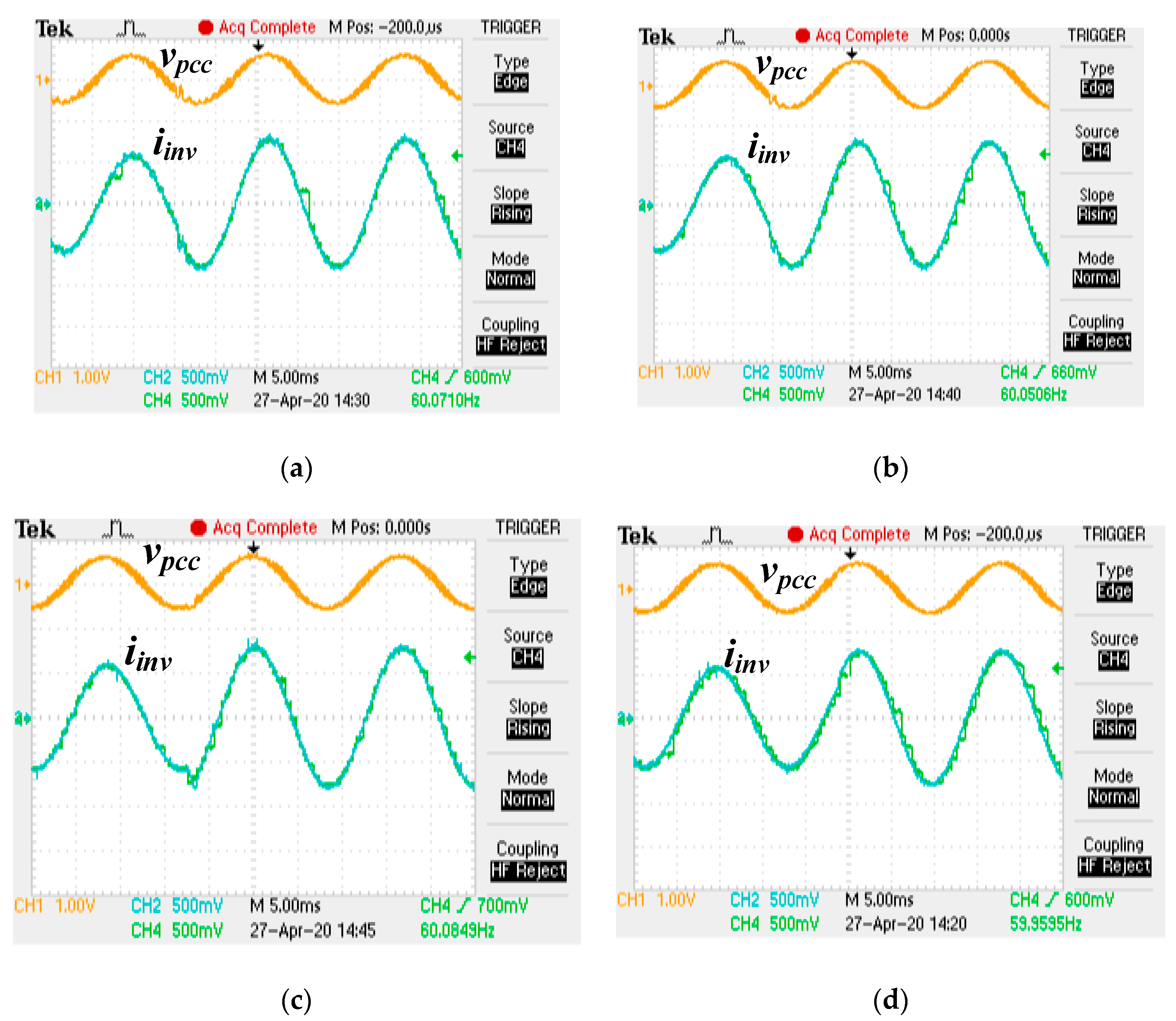
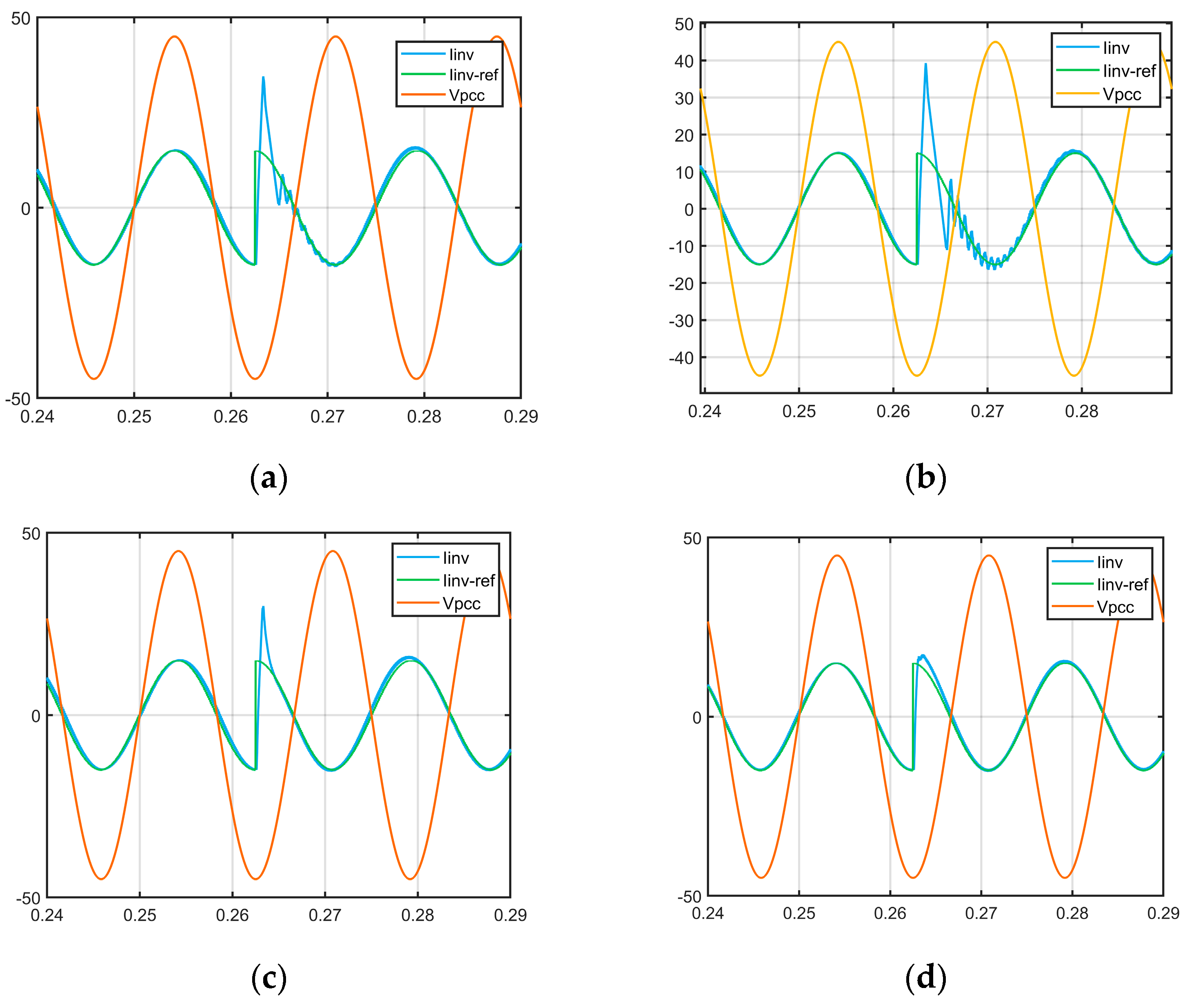
Figure 14 presents the PCC voltage, the inverter output current, and its reference signal during a step in the reference signal from 0.75 to 1 pu. All controllers showed accurate performance, not presenting overshot and oscillatory behavior.
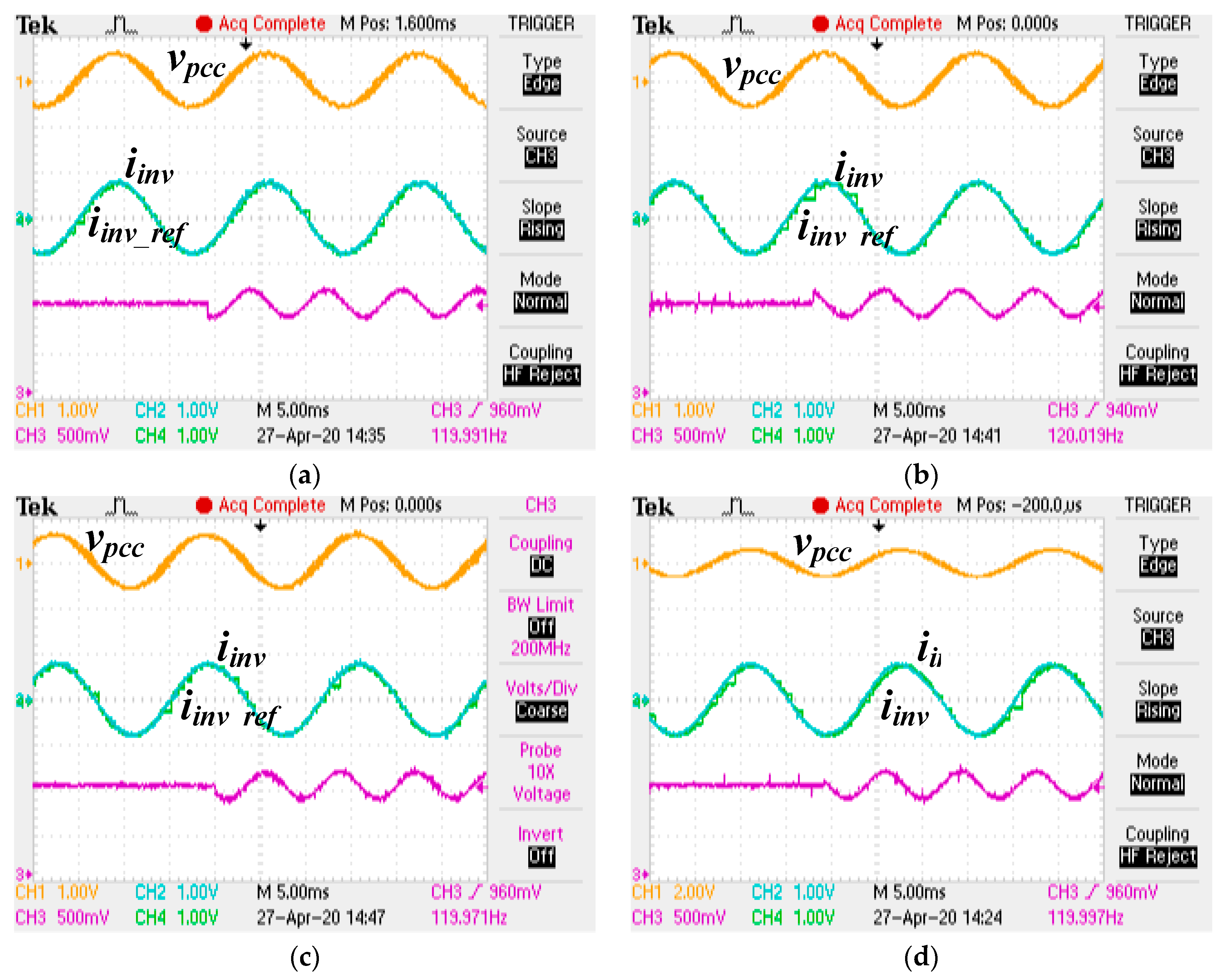
Figure 15 present the PCC voltage, the inverter output current, its reference signal, and the DC voltage during the inclusion of oscillation at the DC link. The oscillation has 10% of the DC voltage and 120 Hz. The output current keeps following its reference signal, as the oscillation was inexistent. This scenario may represent a malfunction in the PV plus DC-DC converter that is connected to the DC link of the LCL-filter inverter or the inevitable double-frequency pulsation in single-phase systems. Even in these cases, the results show the ability of the proposed controller to keep working accurately.
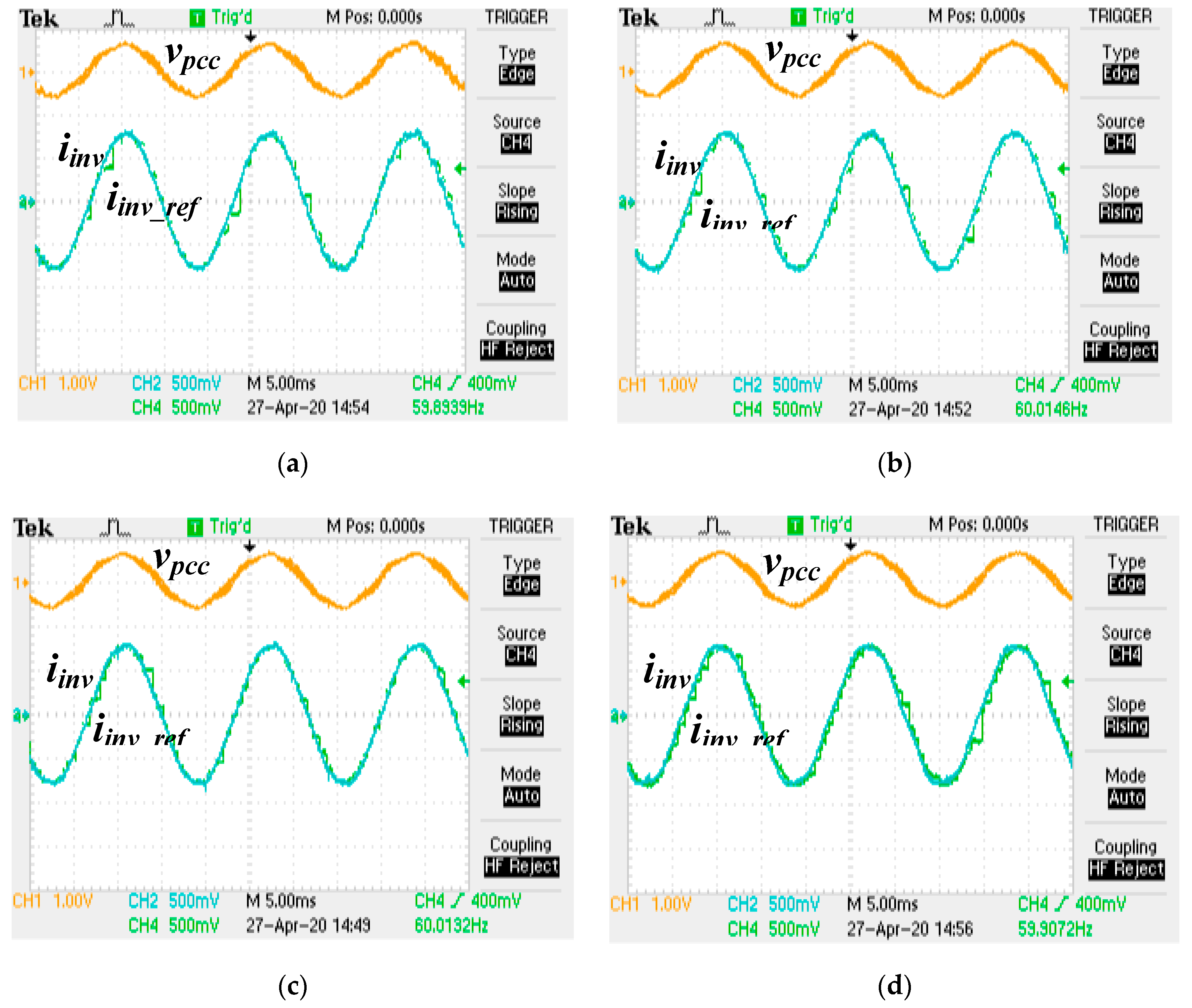
The PCC voltage with harmonic distortion is more and more common in the power distribution system. Figure 16 shows the PCC voltage, the inverter output current, and its reference signal when the grid voltage has 5% related to the fundamental at the fifth harmonic. The controllers keep following their reference signal.
6. Discussion
This section discusses some relevant extra issues of the proposed research. The first is the evaluation of the controllers under bidirectional power flow. Figure 17 presents results when the reference signal for the output current changes its phase related to the PCC voltage. Initially, the current is sinusoidal and in phase with the PCC voltage. Then, the reference signal suffers a 180-degree phase shift. After the transitory interval, the output current returns to follow its reference with negligible steady-state error. Before the transition in the reference, the inverter was injecting active power into the grid. After, the inverter is consuming power from the grid. The inverter output current for the four controllers shows similar behavior as those found during initialization. No unpredictable behavior or instability was observed, indicating that the controllers designed using the proposed procedures were efficient for bidirectional power applications.
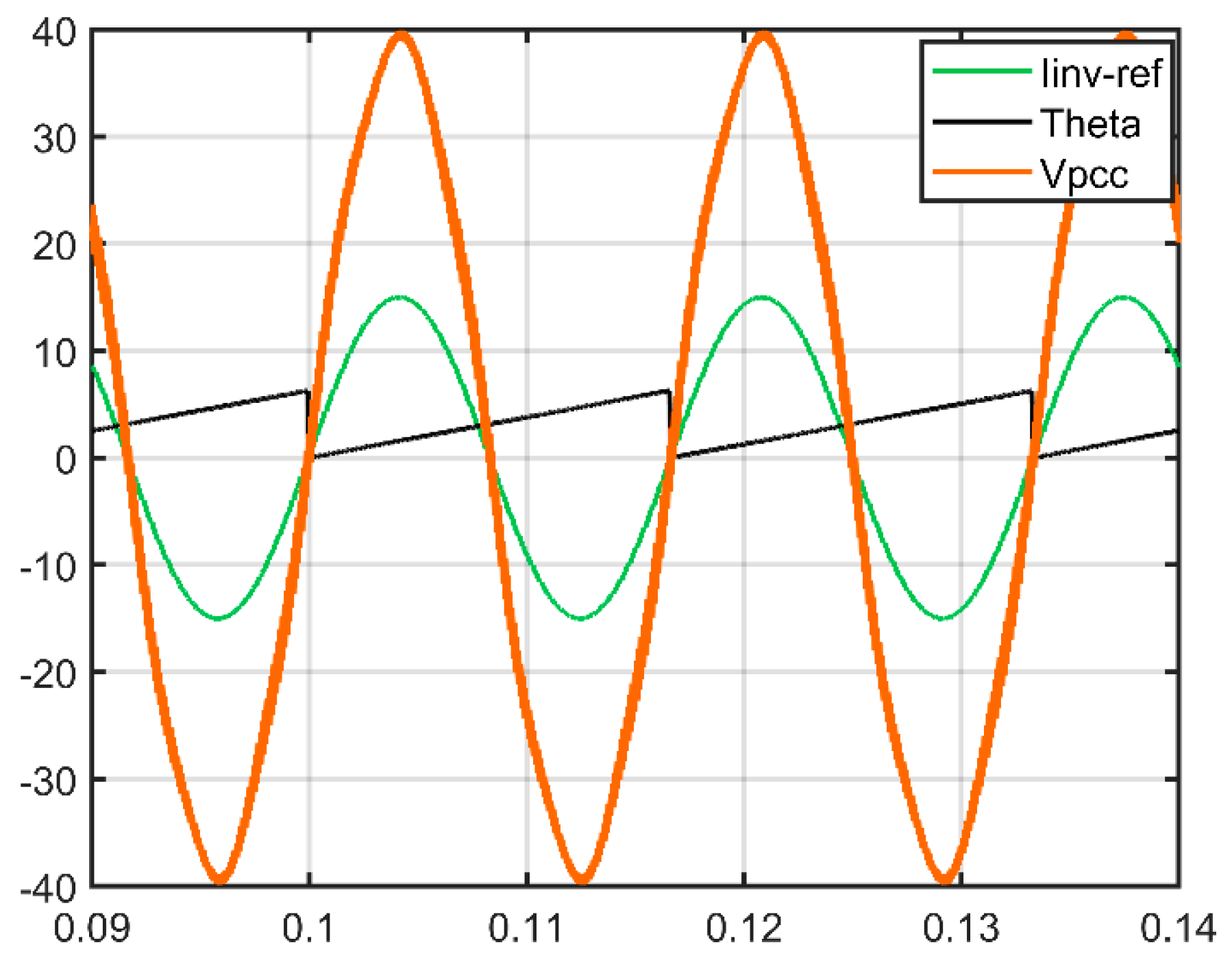
The second topic is the performance of the PLL. Figure 18 shows the PCC voltage, the current reference signal, and the theta signal of the PLL with 5% related to the fundamental at the fifth harmonic. The theta signal, as well as the reference signal for the inverter output current, is clean even in the presence of harmonics. The reference signal is purely sinusoidal. This shows that the PLL employed in this paper was enough to operate under distorted voltage grids.
Another topic that deservers discussion is the frequency of the grid where the inverter is connected. Even though the procedures proposed in this paper used 60 Hz as frequency of the grid, their equations were valid to grid with 50 Hz as well. Attention must be paid to design the PR controller, in which the tuned frequency must be 50 Hz. Moreover, it is attractive to choose the frequency and sampling frequency as multiple of the grid frequency. This makes the ratio between the switching frequency and the grid frequency an integer number, which avoids loss of information during programming the DSC.
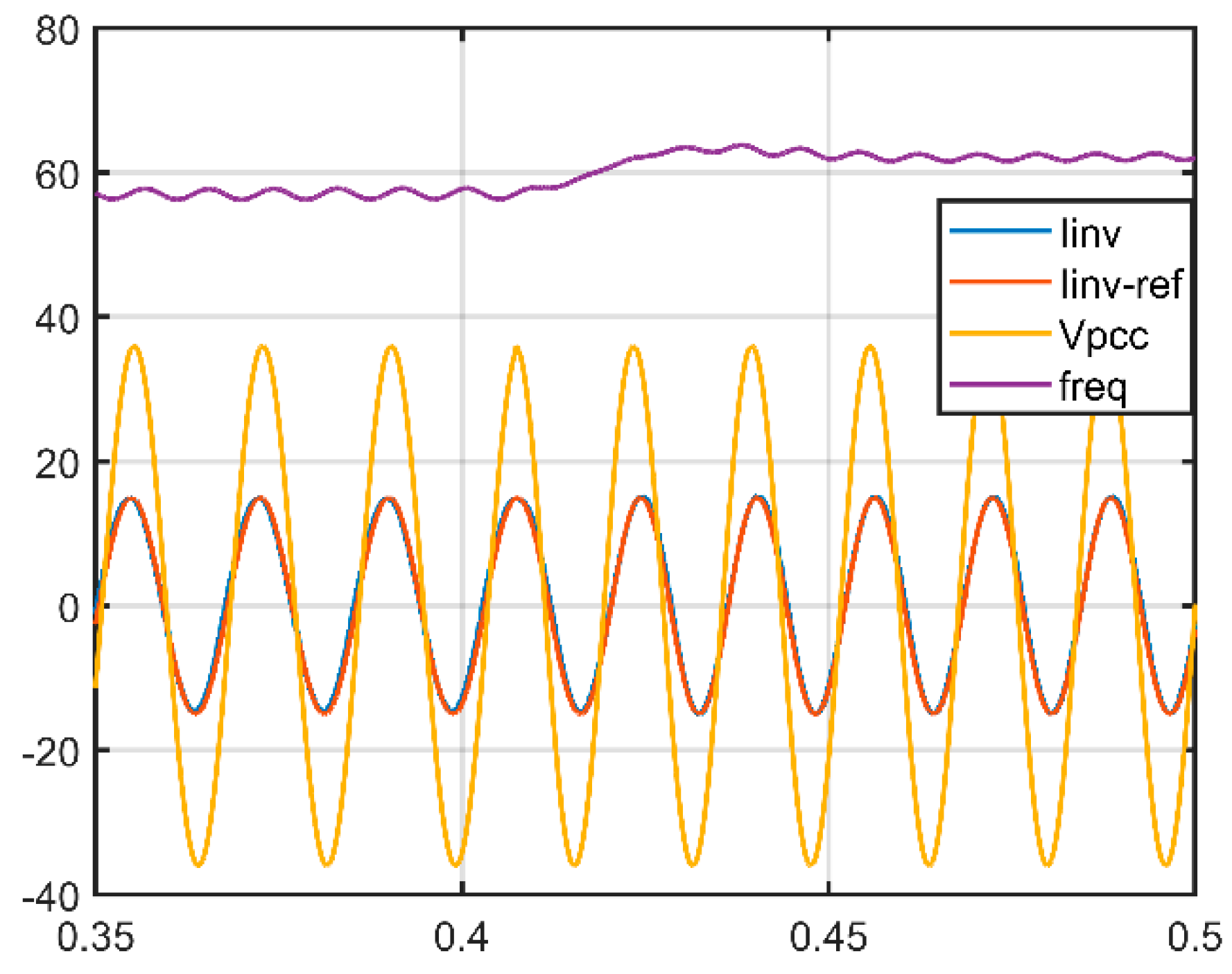
Weak grids often experience frequency variation at the PCC. Consequently, a grid-connected inverter must be able to work under frequency variation conditions. Depending on the deviation of the frequency value, the inverter must either switch off or keep working [3]. Concerning the four controllers proposed in this paper, the PR is the more sensitive for frequency variation. In order to make a PR able to track the frequency variation at the PCC, its parameter tuning procedure needs to be adaptive. Adaptive approaches were beyond the scope of this paper. However, the PR designed in this paper as well as the PLL can work under frequency variation. This is due to the non-null bandwidth of them. Figure 19 shows the PCC voltage, the inverter output current, its reference signal, and the frequency measurement of the PLL during a transition in the frequency of the PCC from 57 to 62 Hz. Such a variation is one of the most severe in weak grids and their limits may not last for more than seconds. The inverter output current keeps following its reference signal with negligible steady-state error. The oscillation in the frequency measurement was expected because the PLL is designed to work at 60 Hz. This oscillation does not compromise the performance of the controller. Therefore, the proposed PR controller is able to work satisfactorily in a weak grid with frequency variation.
7. Conclusions
This paper prosed highly accurately digital current controllers for LCL-filtered grid-connected inverters. The current controllers were the integral single-lead, integral double-lead, integral double-lead taking into account the effect of PWM delay, and the PR. A step-by-step procedure for each one was carefully presented and investigated. Later, the controllers were designed, and the Bode diagram showed the achievement of pre-specified desired parameters.
The proposed controllers were implemented in a physical DSC TMS320F28335 while the power structure was run in the HIL 402 (Typhoon HIL Inc., Novi Sad, Serbia). Results showed the accurate performance of the controller in making the inverter output current follow its reference signal with a steady-state null error. The controlled variables did not show either oscillatory or unpredictable behavior. Therefore, the controllers proposed in this paper are attractive solutions for single-phase LCL-filtered grid-connected inverters. Moreover, the tuning procedures are an easy, fast, and accurate way to design the proposed digital current controllers.
Author Contributions
T.D.C.B. proposed the main idea of this research. He prepared the formulation, the simulation, and the settings of the HIL under the supervision of M.G.S. Additionally, T.D.C.B. ran, collected the results, and wrote this paper while M.G.S. and K.Z. revised it. All the authors were involved in preparing the submitted version of this manuscript. All authors have read and agreed to the published version of the manuscript.
Funding
This research was funded by National Council for Scientific and Technological Development—CNPq Brazil under Grant 421281/2016-2.
Conflicts of Interest
The authors declare no conflict of interest.
References
- Al-Shetwi, A.Q.; Hannan, M.A.; Jern, K.P.; Alkahtani, A.A.; PG Abas, A.E. Power Quality Assessment of Grid-Connected PV System in Compliance with the Recent Integration Requirements. Electronics 2020, 9, 366. [Google Scholar] [CrossRef] [Green Version]
- Zeb, K.; Khan, I.; Uddin, W.; Khan, M.A.; Sathishkumar, P.; Busarello, T.D.C.; Ahmad, I.; Kim, H.J. A Review on Recent Advances and Future Trends of Transformerless Inverter Structures for Single-Phase Grid-Connected Photovoltaic Systems. Energies 2018, 11, 1968. [Google Scholar] [CrossRef] [Green Version]
- Yang, Y.; Kim, K.A.; Blaabjerg, F.; Sangwongwanich, A. Advances in Grid-Connected Photovoltaic Power Conversion Systems; Woodhead Publishing: Dukford, UK, 2018; ISBN 978-0-08-102340-2. [Google Scholar]
- Bao, C.; Ruan, X.; Wang, X.; Li, W.; Pan, D.; Weng, K. Step-by-Step Controller Design for LCL-Type Grid-Connected Inverter with Capacitor–Current-Feedback Active-Damping. IEEE Trans. Power Electron. 2014, 29, 1239–1253. [Google Scholar] [CrossRef]
- Busarello, T.D.C.; Pomilio, J.A.; Simoes, M.G. Design Procedure for a Digital Proportional-Resonant Current Controller in a Grid Connected Inverter. In Proceedings of the 2018 IEEE 4th Southern Power Electronics Conference (SPEC), Singapore, 10–13 December 2018; pp. 1–8. [Google Scholar] [CrossRef]
- Zeb, K.; Islam, S.U.; Din, W.U.; Khan, I.; Ishfaq, M.; Busarello, T.D.C.; Ahmad, I.; Kim, H.J. Design of Fuzzy-PI and Fuzzy-Sliding Mode Controllers for Single-Phase Two-Stages Grid-Connected Transformerless Photovoltaic Inverter. Electronics 2019, 8, 520. [Google Scholar] [CrossRef] [Green Version]
- Espi, J.M.; Castello, J. Capacitive Emulation Using Predictive Current Control in LCL-Filtered Grid-Connected Converters to Mitigate Grid Current Distortion. Energies 2018, 11, 1421. [Google Scholar] [CrossRef] [Green Version]
- Chen, X.; Wu, W.; Gao, N.; Liu, J.; Chung, H.S.-H.; Blaabjerg, F. Finite Control Set Model Predictive Control for an LCL-Filtered Grid-Tied Inverter with Full Status Estimations under Unbalanced Grid Voltage. Energies 2019, 12, 2691. [Google Scholar] [CrossRef] [Green Version]
- Blaabjerg, F. Control of Power Electronic Converters and Systems; Academic Press: London, UK, 2018; Volume 1, ISBN 978-0-12-805436-9. [Google Scholar]
- Wang, X.; Liu, Y.; Zhang, X.; Yang, Q.; Zhang, C. Research on Novel Control Strategy for Grid-Connected Inverter Suitable for Wide-Range Grid Impedance Variation. Electronics 2020, 9, 623. [Google Scholar] [CrossRef] [Green Version]
- Zeb, K.; Din, W.U.; Khan, M.A.; Khan, A.; Younas, U.; Busarello, T.D.C.; Kim, H.J. Dynamic Simulations of Adaptive Design Approaches to Control the Speed of an Induction Machine Considering Parameter Uncertainties and External Perturbations. Energies 2018, 11, 2339. [Google Scholar] [CrossRef] [Green Version]
- Yang, L.; Feng, C.; Liu, J. Control Design of LCL Type Grid-Connected Inverter Based on State Feedback Linearization. Electronics 2019, 8, 877. [Google Scholar] [CrossRef] [Green Version]
- Islam, S.U.; Zeb, K.; Din, W.U.; Khan, I.; Ishfaq, M.; Busarello, T.D.C.; Kim, H.J. Design of a Proportional Resonant Controller with Resonant Harmonic Compensator and Fault Ride Trough Strategies for a Grid-Connected Photovoltaic System. Electronics 2018, 7, 451. [Google Scholar] [CrossRef] [Green Version]
- Zheng, C.; Liu, Y.; Liu, S.; Li, Q.; Dai, S.; Tang, Y.; Zhang, B.; Mao, M. An Integrated Design Approach for LCL-Type Inverter to Improve Its Adaptation in Weak Grid. Energies 2019, 12, 2637. [Google Scholar] [CrossRef] [Green Version]
- Jeong, H.; Lee, J.S. A Stationary Reference Frame Current Control Algorithm for Improvement of Transient Dynamics of a Single Phase Grid Connected Inverter. Electronics 2020, 9, 722. [Google Scholar] [CrossRef]
- Faria, J.; Fermeiro, J.; Pombo, J.; Calado, M.; Mariano, S. Proportional Resonant Current Control and Output-Filter Design Optimization for Grid-Tied Inverters Using Grey Wolf Optimizer. Energies 2020, 13, 1923. [Google Scholar] [CrossRef] [Green Version]
- Lee, S.; Kim, J. Optimized Modeling and Control Strategy of the Single-Phase Photovoltaic Grid-Connected Cascaded H-bridge Multilevel Inverter. Electronics 2018, 7, 207. [Google Scholar] [CrossRef] [Green Version]
- Tang, H.; Zhao, R.; Tang, S.; Zeng, Z. Linear quadratic optimal control of a single-phase grid-connected inverter with an LCL filter. In Proceedings of the 2012 IEEE International Symposium on Industrial Electronics, Hangzhou, China, 28–31 May 2012; pp. 372–376. [Google Scholar]
- Dragoun, J.; Šmídl, V. Adaptive control of LCL filter with time-varying parameters using reinforcement learning. In Proceedings of the IECON 2019-45th Annual Conference of the IEEE Industrial Electronics Society, Lisbon, Portugal, 14–17 October 2019; Volume 1, pp. 267–272. [Google Scholar]
- Arab, N.; Vahedi, H.; Al-Haddad, K. LQR Control of Single-Phase Grid-Tied PUC5 Inverter With LCL Filter. IEEE Trans. Ind. Electron. 2020, 67, 297–307. [Google Scholar] [CrossRef]
- Tang, X.; Chen, W.; Zhang, M. A Current Decoupling Control Scheme for LCL-Type Single-Phase Grid-Connected Converter. IEEE Access 2020, 8, 37756–37765. [Google Scholar] [CrossRef]
- Busarello, T.D.C.; Zeb, K.; Péres, A.; Oruganti, V.S.R.V.; Simões, M.G. Designing a Second Order Generalized Integrator Digital Phase Locked Loop based on a Frequency Response Approach. In Proceedings of the 2019 IEEE PES Innovative Smart Grid Technologies Conference-Latin America (ISGT Latin America), Gramado, Brazil, 15–18 September 2019; pp. 1–6. [Google Scholar]
- Tan, G.; Zong, C.; Sun, X. Tan-Sun Transformation-Based Phase-Locked Loop in Detection of the Grid Synchronous Signals under Distorted Grid Conditions. Electronics 2020, 9, 674. [Google Scholar] [CrossRef] [Green Version]
- Teodorescu, R.; Liserre, M.; Rodriguez, P. Grid Converters for Photovoltaic and Wind Power Systems; John Wiley & Sons: Hoboken, NJ, USA, 2011; ISBN 978-1-119-95720-1. [Google Scholar]
- Buso, S.; Mattavelli, P. Digital Control in Power Electronics, 2nd ed.; Morgan & Claypool Publishers: San Rafael, CA, USA, 2015; ISBN 978-1-62705-754-7. [Google Scholar]
- Rodriguez, J.; Kazmierkowski, M.P.; Espinoza, J.R.; Zanchetta, P.; Abu-Rub, H.; Young, H.A.; Rojas, C.A. State of the Art of Finite Control Set Model Predictive Control in Power Electronics. IEEE Trans. Ind. Inform. 2013, 9, 1003–1016. [Google Scholar] [CrossRef]
- Jun, E.-S.; Park, S.; Kwak, S. Model Predictive Current Control Method with Improved Performances for Three-Phase Voltage Source Inverters. Electronics 2019, 8, 625. [Google Scholar] [CrossRef] [Green Version]
- Ogata, K. Discrete-Time Control Systems; Prentice-Hall International: Upper Saddle River, NJ, USA, 1995; ISBN 978-0-13-328642-7. [Google Scholar]
- Han, Y.; Yang, M.; Li, H.; Yang, P.; Xu, L.; Coelho, E.A.A.; Guerrero, J.M. Modeling and Stability Analysis of $LCL$ -Type Grid-Connected Inverters: A Comprehensive Overview. IEEE Access 2019, 7, 114975–115001. [Google Scholar] [CrossRef]
- Ruan, X.; Wang, X.; Pan, D.; Yang, D.; Li, W.; Bao, C. Control Techniques for LCL-Type Grid-Connected Inverters; Springer: Berlin/Heidelberg, Germany, 2017; ISBN 978-981-10-4277-5. [Google Scholar]
- Mortezaei, A.; Simões, M.G.; Busarello, T.D.C.; Marafão, F.P.; Al-Durra, A. Grid-Connected Symmetrical Cascaded Multilevel Converter for Power Quality Improvement. IEEE Trans. Ind. Appl. 2018, 54, 2792–2805. [Google Scholar] [CrossRef] [Green Version]
- Kazimierczuk, M.K. Pulse-Width Modulated DC-DC Power Converters; John Wiley & Sons: Hoboken, NJ, USA, 2008; ISBN 978-0-470-69465-7. [Google Scholar]
- Busarello, T.D.C.; Mortezaei, A.; Paredes, H.K.M.; Al-Durra, A.; Pomilio, J.A.; Simões, M.G. Simplified Small-Signal Model for Output Voltage Control of Asymmetric Cascaded H-Bridge Multilevel Inverter. IEEE Trans. Power Electron. 2018, 33, 3509–3519. [Google Scholar] [CrossRef] [Green Version]
- Venable, H.D. The K-Factor: A New Mathematical Tool for Stability Analysis and Synthesis. Available online: http://citeseerx.ist.psu.edu/viewdoc/download?doi=10.1.1.196.6850&rep=rep1&type=pdf (accessed on 28 July 2020).
- Bacha, S.; Munteanu, I.; Bratcu, A.I. Power Electronic Converters Modeling and Control: With Case Studies; Springer Science & Business Media: London, UK, 2013; ISBN 978-1-4471-5478-5. [Google Scholar]
Figure 1.
Simplified diagram of the single-phase LCL-filtered grid-connected inverter.

Figure 2.
Simplified diagram of the control strategy.

Figure 3.
Techniques for tuning a digital controller.

Figure 4.
Comparison of the transfer functions that relates to the grid-side current and the inverter duty-cycle considering passive and active damping.
Figure 4.
Comparison of the transfer functions that relates to the grid-side current and the inverter duty-cycle considering passive and active damping.

Figure 5.
Bode diagram indicating the points for phase and the gain at the desired cutoff frequency.
Figure 5.
Bode diagram indicating the points for phase and the gain at the desired cutoff frequency.

Figure 6.
Relation between lead phase versus the K-factor for the integral single-lead and integral double lead controllers.
Figure 6.
Relation between lead phase versus the K-factor for the integral single-lead and integral double lead controllers.

Figure 7.
OLTF for both considering and not considering the effect of the PWM delay.

Figure 8.
Block diagram of how the digital PR controller is implemented.

Figure 9.
Frequency response of the designed digital current controllers.

Figure 10.
Bode diagrams of the designed current controller in s-domain and in z-domain: (a) Integral-single-lead, (b) integral double-loop, (c) integral double-loop considering the PWM delay effect, and (d) resonant filter.
Figure 10.
Bode diagrams of the designed current controller in s-domain and in z-domain: (a) Integral-single-lead, (b) integral double-loop, (c) integral double-loop considering the PWM delay effect, and (d) resonant filter.

Figure 11.
Bode diagram for the closed-loop transfer function considering the designed current controllers.
Figure 11.
Bode diagram for the closed-loop transfer function considering the designed current controllers.

Figure 12.
Experimental and HIL verification: (a) Simplified diagram (b) picture.

Figure 13.
PCC voltage, the inverter output current, and its reference signal during initialization for: (a) Integral-single-lead controller, (b) integral double-lead controller, (c) integral double-lead controller considering the PWM delay effect, and (d) PR controller. (Ch1: 360 V/V; Ch2: Ch4: 20 A/V).


Figure 14.
PCC voltage, the inverter output current, and its reference signal during a step in the reference signal from 0.75 to 1 pu: (a) Integral-single-lead controller, (b) integral double-lead controller, (c) integral double-lead controller considering the PWM delay effect, and (d) PR controller. (Ch1: 360 V/V; Ch2: Ch4: 20 A/V).

Figure 15.
PCC voltage, the inverter output current, its reference signal, and the DC voltage during the inclusion of oscillation at the DC link: (a) Integral-single-lead controller, (b) integral double-lead controller, (c) integral double-lead controller considering the PWM delay effect, and (d) PR controller. (Ch1: 360 V/V; Ch2: Ch4: 20A/V; Ch3: 225 V/V).

Figure 16.
The PCC voltage, the inverter output current, and its reference signal when the grid voltage has 5% related to the fundamental at the fifth harmonic: (a) Integral-single-lead controller, (b) integral double-lead controller, (c) integral double-lead controller considering the PWM delay effect, and (d) PR controller. (Ch1: 360V/V; Ch2: Ch4: 20A/V).

Figure 17.
The PCC voltage (divided by 4), the inverter output current, and its reference signal when bidirectional power flow is investigated: (a) Integral-single-lead, (b) integral double-loop, (c) integral double-loop considering the PWM delay effect, and (d) resonant filter.
Figure 17.
The PCC voltage (divided by 4), the inverter output current, and its reference signal when bidirectional power flow is investigated: (a) Integral-single-lead, (b) integral double-loop, (c) integral double-loop considering the PWM delay effect, and (d) resonant filter.

Figure 18.
The PCC voltage (divided by 4.5), the current reference signal, and the theta signal of the PLL with 5% related to the fundamental at the fifth harmonic.
Figure 18.
The PCC voltage (divided by 4.5), the current reference signal, and the theta signal of the PLL with 5% related to the fundamental at the fifth harmonic.

Figure 19.
The PCC voltage (divided by 5), the inverter output current, its reference signal, and the frequency measurement of the PLL during a transition in the frequency of the PCC from 57 to 62 Hz.
Figure 19.
The PCC voltage (divided by 5), the inverter output current, its reference signal, and the frequency measurement of the PLL during a transition in the frequency of the PCC from 57 to 62 Hz.


Table 1.
System parameters.
| Parameter | Value | Unit |
|---|---|---|
| Grid Voltage | 127 | Vrms |
| Grid frequency | 60 | Hz |
| Converter-side inductor | 2.28 | mH |
| Converter-side resistance | 0.01 | Ω |
| Grid-side inductor | 990 | uH |
| Grid-side resistance | 0.01 | Ω |
| LCL capacitance | 1.64 | uF |
| LCL damping resistance | 20.5 | Ω |
| DC-link voltage | 220 | V |
| Grid resistance | 2 | Ω |
| Grid inductance | 3 | mH |
| Current sensor gain | 0.1 | V/A |
| Switching frequency | 10 | kHz |
| Sampling period | 1 × 10⁻⁴ | s |
| Amplitude of the carrier | 1 | V |
| Desired cut-off frequency | 1250 | Hz |
| Desired phase margin | 60 |
Table 2.
Coefficients of the designed digital current controllers.
| Coefficient | ||||
|---|---|---|---|---|
| - | 0 | - | ||
| - | - | |||
| - | - | - | ||
| - | - | - |
© 2020 by the authors. Licensee MDPI, Basel, Switzerland. This article is an open access article distributed under the terms and conditions of the Creative Commons Attribution (CC BY) license (http://creativecommons.org/licenses/by/4.0/).
Share and Cite
MDPI and ACS Style
Curi Busarello, T.D.; Zeb, K.; Simões, M.G. Highly Accurate Digital Current Controllers for Single-Phase LCL-Filtered Grid-Connected Inverters. Electricity 2020, 1, 12-36. https://0-doi-org.brum.beds.ac.uk/10.3390/electricity1010002
AMA Style
Curi Busarello TD, Zeb K, Simões MG. Highly Accurate Digital Current Controllers for Single-Phase LCL-Filtered Grid-Connected Inverters. Electricity. 2020; 1(1):12-36. https://0-doi-org.brum.beds.ac.uk/10.3390/electricity1010002
Chicago/Turabian StyleCuri Busarello, Tiago Davi, Kamran Zeb, and Marcelo Godoy Simões. 2020. "Highly Accurate Digital Current Controllers for Single-Phase LCL-Filtered Grid-Connected Inverters" Electricity 1, no. 1: 12-36. https://0-doi-org.brum.beds.ac.uk/10.3390/electricity1010002