An Innovative Tunable Rule-Based Strategy for the Predictive Management of Hybrid Microgrids

Abstract

This work proposes a methodology for the optimal training of rule-based management strategies, to be directly implemented in the industrial controller of hybrid off-grid microgrids. The parameters defining the control rules are optimally tuned resorting to different evolutionary algorithms, based on the expected operating conditions. The performance of the resulting management heuristics is compared with conventional approaches to optimal scheduling, including Mixed Integer Linear Programming (MILP) optimization, direct evolutionary scheduling optimization, and traditional non-trained heuristics. Results show how the trained heuristics achieve a performance very close to the global optimum found by the MILP solution, outperforming the other methods, and providing a single-layer commitment and dispatch algorithm which is easily deployable in the microgrid controller.

1. Introduction

Microgrids [1] have catalyzed increasingly vast attention in recent years. The technological advancements involving many distributed energy resources have fostered their evolution: from straightforward isolated systems, supplying electricity in remote areas mainly relying on diesel generators, to more articulated structures, that can ensure improved economic performances, lower environmental impact, and have a broader range of applicability. This is made possible by a more pervasive presence of distributed energy resources and their increasing remote control capability, which allows the integration of generators, storages and flexible loads [2] in coordinated control systems. Of particular interest is the case of hybrid microgrids, which combine traditional dispatchable generators with electrochemical storage systems and Renewable Energy Sources (RES), such as PV panels and wind turbine generators [3,4,5]. These systems are expected to play a significant role in the electrification of regions where the national grid is poorly developed or unreliable [6], as they can serve as cost-effective nucleation centers for increasingly interconnected local electrical networks.

The management strategy adopted in the microgrid has a substantial effect on its performance, as it is responsible for reducing fuel consumption as much as possible, maximizing the exploitation of RES, and determining the strategic usage of the energy storage systems. Two main classes of management approaches can be identified:

• Rule-based strategies: decisions are taken based on a predefined response pattern to a set of monitored conditions (e.g., net demand, storage state of charge);
• Predictive optimization: scheduling decisions are the variables of an optimization problem, defined over a given future temporal window;

Rule-based strategies have been traditionally adopted, especially in off-grid systems, due to their simplicity and effectiveness. The most well-known examples are the cycle-charge (CC) and load-following (LF) strategies [7], which establish two alternative modes of interaction between dispatchable generators and storage systems in islanded hybrid microgrids. CC and LF have been explored in many works in the literature [8,9,10,11] and are implemented as reference management solution in the commercial software HOMER [12].

Predictive optimization, on the other hand, requires describing the system in terms of its technical constraints and to identify a temporal window over which the scheduling decisions constitute the problem variables [13,14,15]. Different mathematical techniques can then be adopted to solve the optimization problem. Mixed Integer Linear Programming (MILP) based EMS are currently the most used approach, since they can effectively deal with large numbers of integer variables and provide the globally optimal solution [16]. For instance, MILP is applied effectively for the optimal short-term management of a microgrid in [17,18]. However, the on-field application of these techniques is made difficult by the mathematical and numerical complexity of the MILP models, which often require the use of licensed commercial solvers that cannot be handled directly by the microgrid control system architecture typically constituted by Programmable Logic Controllers (PLC) [19,20]. Among all the other possible predictive approaches for EMS in microgrids, Evolutionary Algorithms (EA) have been applied to substitute for the MILP formulation. In [21], the control management of the microgrid is managed by means of Genetic Algorithm (GA), which manages the set point of all the dispatchable generators and the power exchanged by the Energy Storage System. Similarly, in [22], the authors solved the scheduling problem with a hybrid Differential Evolutionary–Harmony Search (DE–HS) algorithm. A slightly different approach is implemented in [23], where the problem constraints have been considered as additional objectives and, thus, the multi-objective problem has been solved with Non-Dominated Sorted Genetic Algorithm-II (NSGA-II). Even if these algorithms allow a non-linear formulation of the problem and overcome the need of expensive software licenses to solve the optimization instance, they do not ensure to reach the global optimum of the objective function and, being computationally expensive both in terms of resources and time, they must rely on a PC hardware. Additionally, any predictive optimization nominal solution should be continuously adjusted by a real-time re-dispatching layer to cope with instantaneous deviations of net demand from forecasts, increasing the complexity of the whole control system.

As far as real-time control is concerned, it is worth noting that EAs have been used for optimization of the parameters of controllers in many works. In [24], the authors propose an optimal parameter setting method that exploits Particle Swarm Optimization for enhancing power quality and load following in island operation conditions. In [25], the authors compare three different optimization algorithms for parameter tuning of a PI controller. In particular, they test Salp Swarm Algorithm (SSA), Particle Swarm Optimization (PSO) and Grasshopper Optimization Algorithm (GOA). Another approach is the use of fuzzy logic for the definition of the controller. In [26], the authors present a Fuzzy Logic Controller (FLC) for the Time-of-Use Cost Management program in the microgrid. The parameters of the FLC are set by means of a Genetic Algorithm. In [27], the authors propose a complex system that combines Neural Networks (NN), GA and Fuzzy Logics (FL) for the optimal management of a microgrid. In particular, NN are used for the forecasting of variable loads and production, while GA and FL are then applied for the optimal microgrid management.

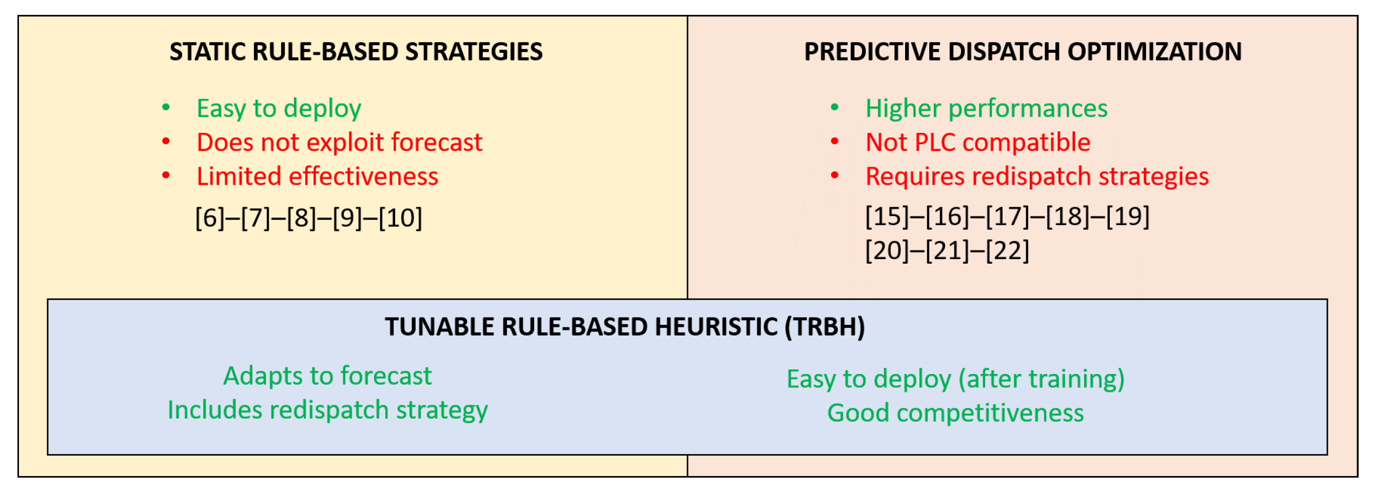
To the best of authors’ knowledge, even if EAs have been already applied for the optimization of real time regulators, they have never been leveraged to tune parameters for rule-based heuristic strategies applied to microgrid management. This work proposes a new methodology for the optimal training of predictive rule-based management strategies, which can attain improved performances with respect to traditional rule-based approaches while still be suited for direct implementation in the microgrid PLC. The parameters of the control heuristics are tuned, resorting to evolutionary algorithms, based on the day-ahead forecast of demand and RES generation potential. The performance of the proposed framework is compared with alternative approaches, including the direct adoption of MILP optimization, evolutionary optimization, and traditional non-trained heuristics. The effect of the uncertainty on the forecasts is not accounted for in this work, so to exclude in the comparison the effect of the adopted re-dispatch algorithm adopted and only compare the dispatch strategies under the assumption of perfect foresight. However, it must be further stressed that one of the advantages of the proposed Tunable Rule-Based Heuristic (TRBH) strategy is that it implicitly provides a re-dispatching strategy, since a specific response can be computed for any arbitrary manifestation of uncertainty according to the optimally tuned dispatch rules. The results show how the trained heuristics achieve performance very close to the direct solution of the MILP formulation, outperforming the other classical rule-based methods, and also intrinsically providing a response pattern to the deviations of exogenous parameters from forecasts. A summary of the advantages of the proposed TRBH method with respect to other management strategy solutions is presented in Figure 1.

The remainder of this paper is organized as follows. The problem statement and the comparison objectives are explained in Section 2. The modelling of system and units is presented in Section 3, followed by the control strategies in Section 4. Simulation results and conclusion remarks are discussed in Section 5 and Section 6, respectively.

2. Problem Description

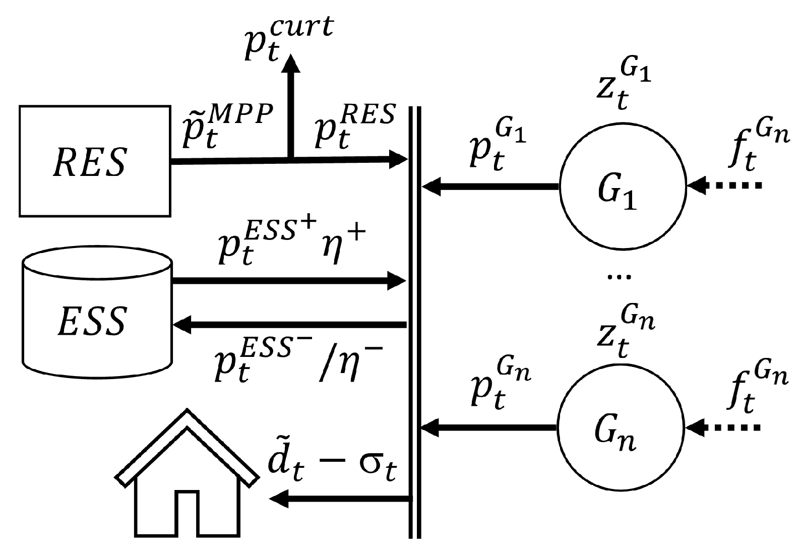
The conceptual schematization of a general hybrid microgrid is represented in Figure 2. The microgrid comprises a set of RES, a set of dispatchable generators, an energy storage system, and an aggregated electrical load. A single-node representation of the microgrid is commonly assumed when defining the optimal scheduling problem: if the electrical connections have a limited extension (e.g., generators and loads are all in the same area) and do not operate close to their maximum capability, the expected voltage profile variance is minimal and voltage regulation does not influence the active power flow. The electrical stability including frequency and voltage regulation can, therefore, be fully entrusted to lower control layers that can be directly managed by the microgrid subunits [28]. Under this assumption, different RES generation technologies can be aggregated in a single power injection term.

Thus, the role of the management strategy is to determine in each time step the scheduling plan, defined by (i) the optimal commitment status $z^G$ (on/off) of all dispatchable generators and (ii) the operating setpoint for all microgrid units.

The competitiveness of a given scheduling solution is measured in terms of overall operating cost, including (i) the cost of fuel, (ii) operation and maintenance costs for all units (including the estimation of components wearing), and (iii) the cost of non-served energy (e.g., cost of service interruptions).

Comparability of Scheduling Approaches

As mentioned, different scheduling approaches are compared in this work, but their applicability is not the same and the terms of the comparison must, therefore, be clarified.

The solution of the MILP formulation of the optimal scheduling problem sets a lower bound for the operating costs, as this optimization technique can certify the global optimality of the solution. The competitiveness of the other methods is, therefore, not related to the quality of the optimal scheduling plan they can identify, but rather to their simpler and cheaper implementation in real-life systems, which might justify a minor reduction in the optimality of the scheduling solution. Specifically, rule-based strategies have null computational cost and can be directly implemented in the system PLC, whereas evolutionary algorithms, even if they require a considerable computational effort and thus a PC-based hardware, do not require the purchase of expensive dedicated commercial solvers.

Furthermore, the MILP and evolutionary scheduling techniques only provide a reference plan associated with the considered forecasts of demand and RES generation. To be used in real-life EMS, these techniques must therefore be complemented by lower control layers, that adjust the dispatch of units to cope with the deviations of exogenous parameters from forecasts. The need for second-layer corrections can most likely cause a performance reduction compared to the perfect forecast assumption, the entity of which also depends on [29]:

• the magnitude of forecast errors;
• how uncertainty was addressed in the problem formulation;
• the quality of the correction algorithm implemented.

The deterministic scheduling solution thus represents a lower bound to the actual operating cost that would follow an accurate quantification of the effect of uncertainty.

Conversely, rule-based strategies can be implemented by simply following the dispatch actions prescribed by the real-time monitoring of demand and RES production and do not need the implementation of any re-dispatching layer.

3. System Modelling

The optimization of scheduling decisions, as well as the evaluation of the system performance associated with different management strategies, is based on a mathematical model of the system operation. MILP optimization requires the modelling equations to be linear, whereas the other methods considered do not impose any restriction on the problem formulation. In the modelling approach conventionally adopted for hybrid microgrid systems, the main non-linearity to be accounted for is represented by the part-load curve of the generators. In the MILP formulation, the curve has been approximated through a piece-wise function. The number of breakpoints of the piecewise has been controlled to ensure a negligible error in the approximation.

The following paragraphs summarize the modelling approach adopted for each microgrid component. All the model parameters have been identified with the hat symbol.

3.1. Dispatchable Generators

Regardless of the technology they are based upon, dispatchable generators are fundamentally represented by their part-load curve, which associates fuel consumption $f_t^G$ to the corresponding rate of output production ($p_t^G$) at a certain time step t. When in operation (commitment status $z_t^G$ equal to 1), the generators must work in the range of admissible operating conditions, defined by their maximum and minimum load (respectively ${\widehat{p}}_{max}^G$ and ${\widehat{p}}_{min}^G$). Other technical constraints include potential limitations in terms of dynamic variation of the operating load (up/downwards ramp rate), and duration of start-up and shut down operations (minimum up/downtime). It has to be noted that since this work deals with hourly simulation time steps, this last constraints have not been included.

3.2. Renewable Generators

The aggregate non-dispatchable RES generator is represented by the overall generation potential profile ${\widehat{p}}_t^{MPP}$, which states the maximum power output that can be extracted by the RES set when working in Maximum Power Point (MPP). The actual output of most renewable generators can be reduced compared to MPP conditions, operating a generation curtailment $p_t^{curt}$ and leading by subtraction to the definition of the net RES contribution $p_t^{RES}$.

3.3. Energy Storage System

A simple dynamic model is considered to describe the evolution of the energy stored in the ESS $So{E}_t$, namely the State of Energy (SoE) at time t, accounting for the power exchange of the ESS with the common bus net of losses due to its charge/discharge efficiencies ${\widehat{\eta }}^{+}$ and ${\widehat{\eta }}^{-}$. $So{E}_t$ is bounded between the maximum and minimum state of energy thresholds (${\widehat{SoE}}_{max}$ and ${\widehat{SoE}}_{min}$). It is worth mentioning that two more constraints are implemented to limit the ESS power between maximum discharge power ${\widehat{p}}_{max}^{ESS}$ and minimum charge power ${\widehat{p}}_{min}^{ESS}$. Despite its simplicity, the model has proven to be adequately accurate for battery technologies such as Li-Ion, which currently represent the dominant technological solution adopted in the hybrid systems under analysis.

3.4. Electrical Load

The microgrid electrical load is modelled as a power absorption profile ${\widehat{d}}_t$, which can be partially reduced by shedding a fraction of the load ${\sigma }_t$. The cost of load shedding is proportional to the amount of non-served energy.

3.5. Spinning Reserve Requirements

To ensure a stable operating schedule, reserve constraints are normally enforced on the operating profiles, imposing that the system can promptly respond to a sudden increase in net demand relying on the currently committed generation resources. The net demand increase can either be caused by a reduction in the non-dispatchable RES generation potential or by an increase in the load energy demand. The contribution of the active dispatchable generators to the system spinning reserve can be computed considering the status of the generator and their maximum load (ramp limitations have not been considered due to the hourly resolution considered during the simulations). The contribution of the ESS is instead determined by its maximum power output and by its available energy content. In formula,

$$\begin{array}{c}S{R}_t=\sum _G^{n_G}S{R}_t^G+S{R}_t^{ESS}>{\widehat{d}}_t(1+\widehat{\gamma })-{\widehat{p}}_t^{MPP}(1-\widehat{\beta })\end{array}$$

(1)

$$\begin{array}{c}S{R}_t^G=z_t^G{\widehat{p}}_{max}^G\end{array}$$

(2)

$$\begin{array}{c}S{R}_t^{ESS}=min\left({\widehat{p}}_{max}^{ESS},\frac{So{E}_t-{\widehat{SoE}}_{min}}{\Delta t}\right)\end{array}$$

(3)

where $n_G$ is the total number of dispatchable generators, $S{R}_t^G$ indicates the spinning reserve contribution of each generator at time t, $S{R}_t^{ESS}$ quantifies the spinning reserve guaranteed by the energy storage, $\widehat{\gamma }$ and $\widehat{\beta }$ identify the increase in load demand and the potential drop in RES power output, respectively.

4. Scheduling Strategies

This section describes the approaches to optimal scheduling compared in this work: deterministic MILP scheduling, evolutionary scheduling, CC and LF strategy scheduling, and the proposed evolutionary training of rule-based heuristics scheduling.

4.1. Milp Scheduling Optimization

A detailed description of the MILP formulation for the scheduling problem of an off-grid microgrid can be found in [4] and, therefore, is not extensively addressed in this work. A deterministic formulation is pursued, including spinning reserve constraints, as specified in Section 3. The solution of the formulation provides an absolute lower bound for the operating cost, which can be used to assess the competitiveness of the other scheduling approaches.

4.2. Evolutionary Scheduling Optimization

The second considered scheduling approach is based on the direct use of Evolutionary Optimization Algorithms (EAs) to tackle the predictive optimal scheduling problem. This class of algorithm is suitable for the solution of high-dimensional non-linear and multimodal problems [30]. Among all the possible EAs, Social Network Optimization (SNO) has been used in this work because of the high-quality performance that this algorithm shows in many problems [31].

The optimization algorithm, in this application, can directly set the power contributions to the system. The total number of management variables required by the EMS is $(n_G+1)\times n_H$, where $n_H$ is the number of hours in the considered time horizon. In fact, for this optimization, as for the MILP scheduling strategy, an hour time discretization has been used. The selection of the effective design variables has been investigated for improving the system performance.

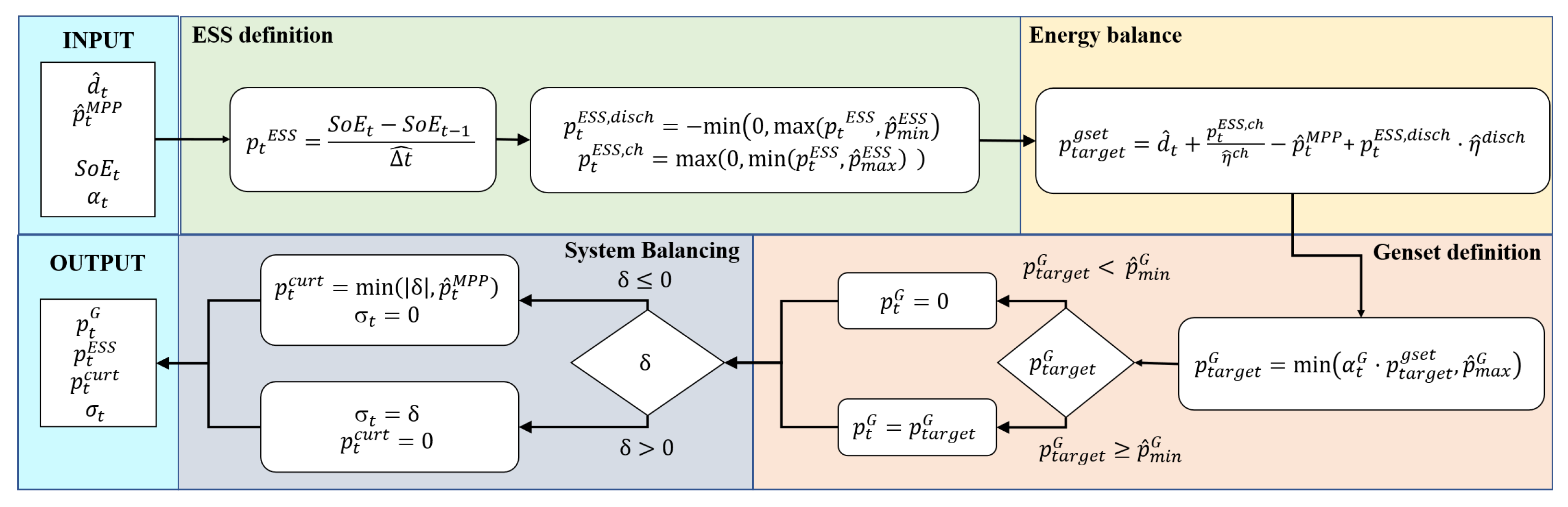
As first step, the energy balance equation has been inserted in the variable decodification phase in order to avoid service interruptions ($\sigma =0$) and reduce the number of free variables. The two remaining degrees of freedom for each time step has been managed as follows. The selected dispatch variables are the battery $SoE$ trajectory and the load sharing coefficients $\alpha$ among the generators. These variables are selected due to their minimal coupling, for helping the optimization stability, and for their matching with the performance parameters.

In fact, the reduced coupling of the variables can be clarified by analysing the problem decodification process shown in Figure 3. The inputs of the system are the scenario information (demand ${\widehat{d}}_t$ and and potential RES production ${\widehat{p}}_t^{MPP}$) and the optimization variables ($SoE$ and $\alpha$).

The first optimization variable (the $SoE$) is used to compute the power exchanged by the ESS (ESS definition block in Figure 3): this step takes into consideration the physical limits of the BESS in terms of power exchangeable. The minimum and the maximum $SoE$, instead, are directly embedded in the optimization process by means of using the absorbing wall boundary condition [32].

The ESS power exchange computed in this way is used to find the target genset production by exploiting the energy balance:

$$p_{target}^{gset}={\widehat{d}}_t+\frac{p_t^{ESS,ch}}{{\widehat{\eta }}^{ch}}-{\widehat{p}}_t^{MPP}-{\widehat{\eta }}^{disch}{p}_t^{ESS,disch}$$

(4)

The target genset production is split among the generator by using the ${\alpha }_t$ values, i.e., the breakdown of this production between the available generators:

$$p_{target}^G=min({\alpha }_t^G·p_{target}^{gset},{\widehat{p}}_{max}^G)$$

(5)

where ${\widehat{p}}_{max}^G$ is the maximum dispatchable power from the generator. This target production is compared with the minimum dispatchable power to find the actual production of generator G:

$$p_t^G=\left\{\begin{array}{cc}0\hfill & p_{target}^G<{\widehat{p}}_{min}^G\hfill \\ p_{target}^G\hfill & p_{target}^G\ge {\widehat{p}}_{min}^G\hfill \end{array}\right.$$

(6)

This approach for the computation of the production from dispatchable generators already takes into account the physical constraints on the generator and, at the same time, reduces the difference between the target genset production and the actual one.

The optimization variables are partially decoupled because the ${\alpha }_t$ value does not interact with the $So{E}_t$ trajectory for the ESS power definition. In addition to this, they have a different effect on the system: the $SoE$ trajectory takes into account almost all the contributions to the power balance, while the $\alpha$ values are devoted to the minimization of the specific consumption of the genset.

The cost function should take into account five different performance parameters. The first one is the actual target of the optimization process, i.e., the total consumption of the genset. The second and the third cost components are related to the two violations of constraints: the absence of service interruptions and the spinning reserve. Both these two constraints are managed by means of a two-stage penalty approach: if they are violated, a constant cost is added to the penalization proportional to the constraint violation. In this way, the unfeasible solutions have an higher cost than feasible ones and the optimizer is driven toward solutions with a lower constraint violation. Finally, the last two cost components are added to further penalize suboptimal solutions: in fact, a cost component is associated to dump production and to curtailed RES.

The selected design variables and the cost definitions help the optimizer in finding good and feasible solutions with a low computational load.

4.3. Load Following and Cycle Charge

Cycle Charge (CC) and Load Following (LF) are two of the widely adopted rule-based strategies that will be considered as a benchmark for this study [12]. CC basically consists of running the dispatchable generators at full load whenever they are in operation, this may result in a surplus of production that is used to recharge the Energy Storage System (ESS). Once the ESS State of Charge (SoC) overcomes a certain level, its discharge is prioritized with respect to the dispatchable generators until the SoC is reduced below a lower threshold. LF on the contrary always prioritizes the ESS over the dispatchable generators, which run at partial load, producing only enough power to meet the net demand, thus, ESS charging is caused only by a surplus of renewable energy.

4.4. Tunable Rule-Based Heuristic Strategy

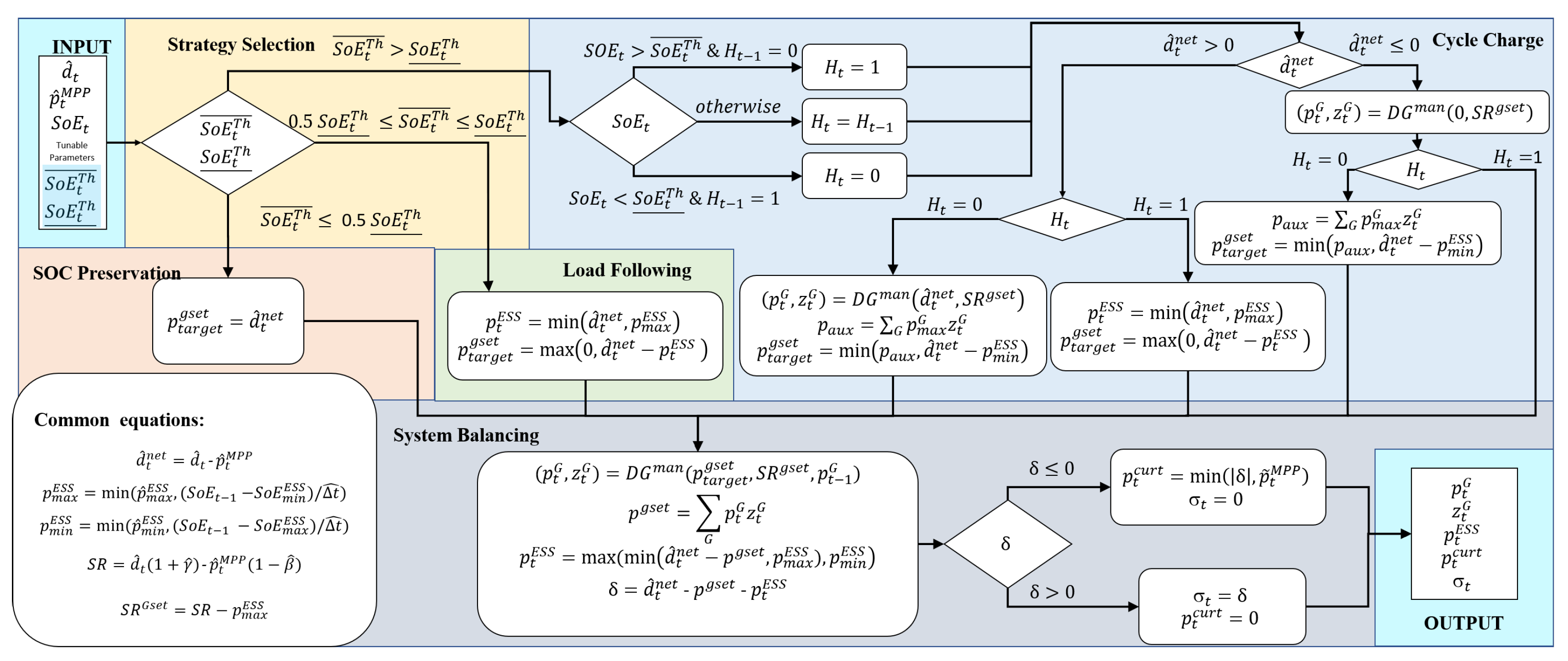
The TRBH strategy we propose in this work is based on the definition of an adaptable superstructure, which can be flexibly configured to define a wide range of operating modes. Dispatch decisions are based on the observed net demand (assuming the operation of RES generators in MPP tracking), while enforcing that an adequate spinning reserve is always available and that all technical limitations on the units are respected. The logical scheme of the described heuristic is shown in Figure 4. It is apparent how the value of SoE thresholds $\overline{So{E}_t^{Th}}$ and $\underline{So{E}_t^{Th}}$ determine the strategic utilization of the ESS. Specifically, three scenarios can be identified:

• If $\overline{So{E}_t^{Th}}\ge \underline{So{E}_t^{Th}}$, the strategy is equivalent to the traditional CC, with the amplitude of the ESS cycles set by the value of the thresholds. In particular, if ${\overline{SoE}}_t^{Th}>{\widehat{SoE}}_{max}^{ESS}$ (maximum allowable SoE) or $\underline{So{E}_t^{Th}}<{\widehat{SoE}}_{min}^{ESS}$ (minimum allowable SoE), the corresponding prioritization mode switch, defined by the the change of variable H that prioritize programmable generators over storages, will not be allowed. In other words, in these conditions, the periodic cycling of the ESS, specific to this control strategy, will be forbidden.
• If $0.5\underline{So{E}_{Th}}\le \overline{So{E}_t^{Th}}\le \underline{So{E}_t^{Th}}$, the strategy is equivalent to the traditional load following (LF): the battery is always prioritized with respect to programmable generators and recharged only if RES production is exceeding demand, while the generators supply positive net loads.
• If $\overline{So{E}_t^{Th}}\le \underline{So{E}_t^{Th}}$, the energy content of the battery is stabilized, following the net load with the generators without discharging the storage. Precisely for this reason, this operating scenario has been classified as SoC Preservation (SP).

The aggregate power generation required from the genset is distributed among the individual generators through a separate dispatch routine, which implements the classic lambda iteration method [33]. In addition to the active power constraint, this routine ensures that the constraints on minimum on and off time and ramp rate requirements of programmable generators are satisfied. This function also guarantees that an adequate spinning reserve is provided to the system. These features are obtained by sorting out all the combinations that respect the aforementioned constraints, applying the lambda method to all the feasible options and selecting the best solution in terms of total fuel consumption.

A final step where the system balance is checked is necessary to manage potential setpoint redistribution to the ESS in case some programmable generator’s constraints are active and to manage potential RES curtailment.

To increase the flexibility of the tunable heuristic strategy, the horizon window is divided into intra-day periods, for which different SoE thresholds can be defined. The daily operating strategy, therefore, results from the combination of different operating modes during different hours of the day. The effect of the number of intra-day windows considered is explored at the end of Section 5.

5. Results

5.1. Case Study Description

The described scheduling strategies are numerically compared by simulating the operation of an off-grid microgrid. Demand and non-dispatchable generation potential profiles have been characterized based on on-field measurements in the real-life microgrid supplying the village of Garowe, Somalia.

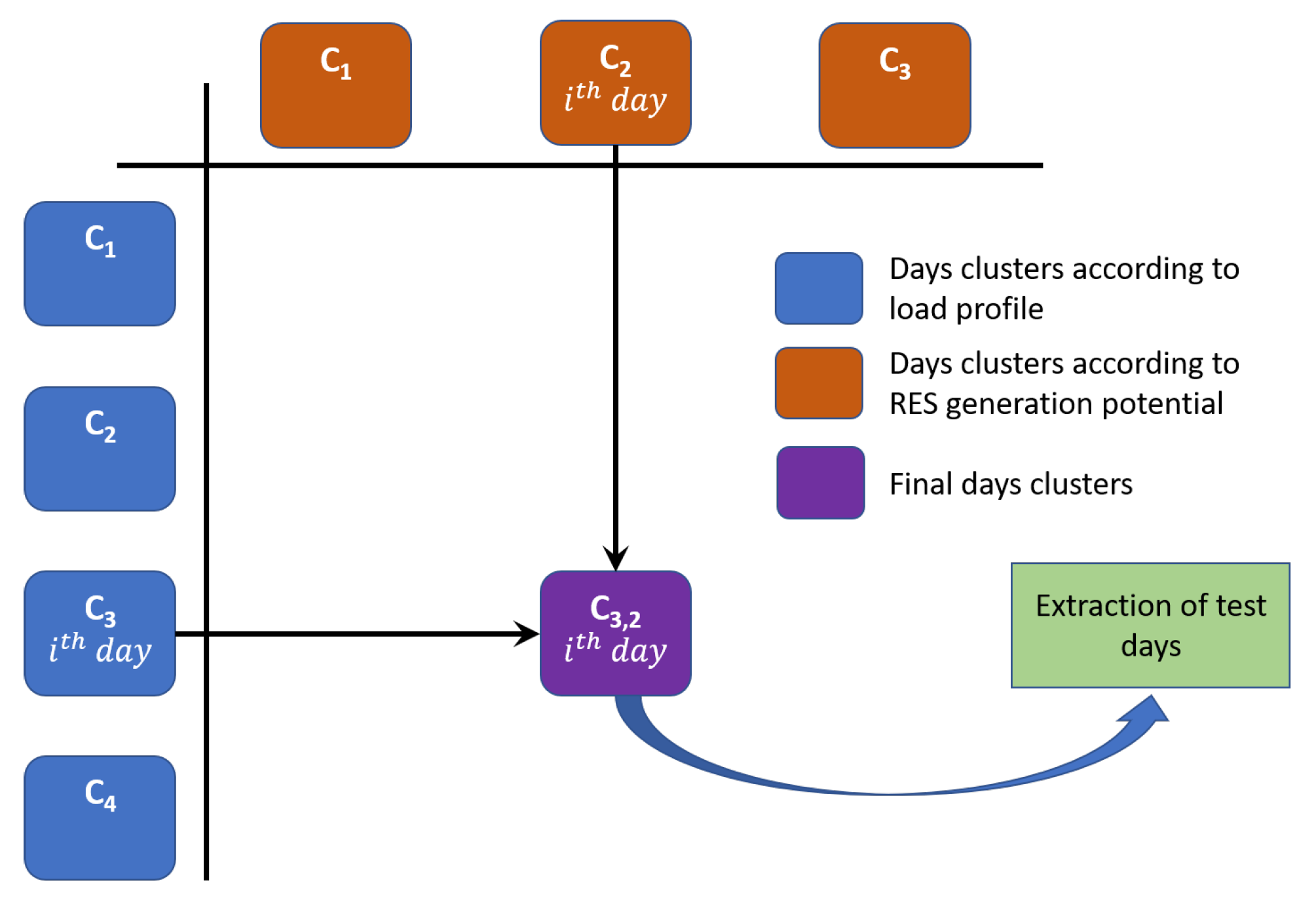
In order to find a set of possible scenarios for assessing the proposed technique, the available dataset has been clustered. Starting from a dataset spanning 12 months with an hourly resolution, the days have been separately clustered in terms of electricity consumption and RES generation potential profiles, identifying, respectively, three and four groups of days through the k-means algorithm (Figure 5: orange and blue clusters, respectively). The Cartesian intersection between the two sets of clusters then defines a resulting redistribution of the initial population of days in twelve new clusters (Figure 5: purple clusters). From these clusters, subsets of days have been extracted for the numerical campaign. To ensure a good balancing of the clusters in the final set of scenarios, the number of days selected from each cluster is proportional to the cluster size; in this way, the sub-set of scenarios is well representative of the original dataset. The final number of test days is 28.

The analysed microgrid for this study is a system comprising of two 550 kW diesel generators, one 1440 kW/1440 kWh storage, and a 1000 kWp PV field.

Simulations were carried out on an Intel(R) Core(TM) i9-10900KF processor, 64 GB RAM computer. All the optimization trials with genetic algorithms use the number of objective function calls as termination criterion: in fact, it is well representative of the total computational time required for the optimization due to the fact that the algorithm self-time is negligible with respect to the total. Each trial of optimization for the TRBH requires around 38 s. This time does not depend on the number of intervals, since they do not influence the computational complexity of the cost evaluation process (although they will impact on the speed of convergence to the optimal solution). To improve performances, ten trials are launched for each test day, leading to a total computational time of 380 s per day. For the pure EA dispatch optimization problem, since it involved a reduced numerical complexity of the cost function evaluation, the average computation time of a single trial of optimization is 5 s, corresponding to 50 for each test day. For the MILP optimization, a convergence gap of 0.1% is considered, associated with an average simulation time of about 4 s per test day. Due to the optimality proof characterizing MILP optimization, no multi-trial approach is necessary.

5.2. Rule-Based Heuristic Structure Optimization Results

The tuning of SoE thresholds defining the TRBH described in Section IV is a non-linear problem that is greatly affected by the specific demand and RES production profiles characterizing the day under analysis.

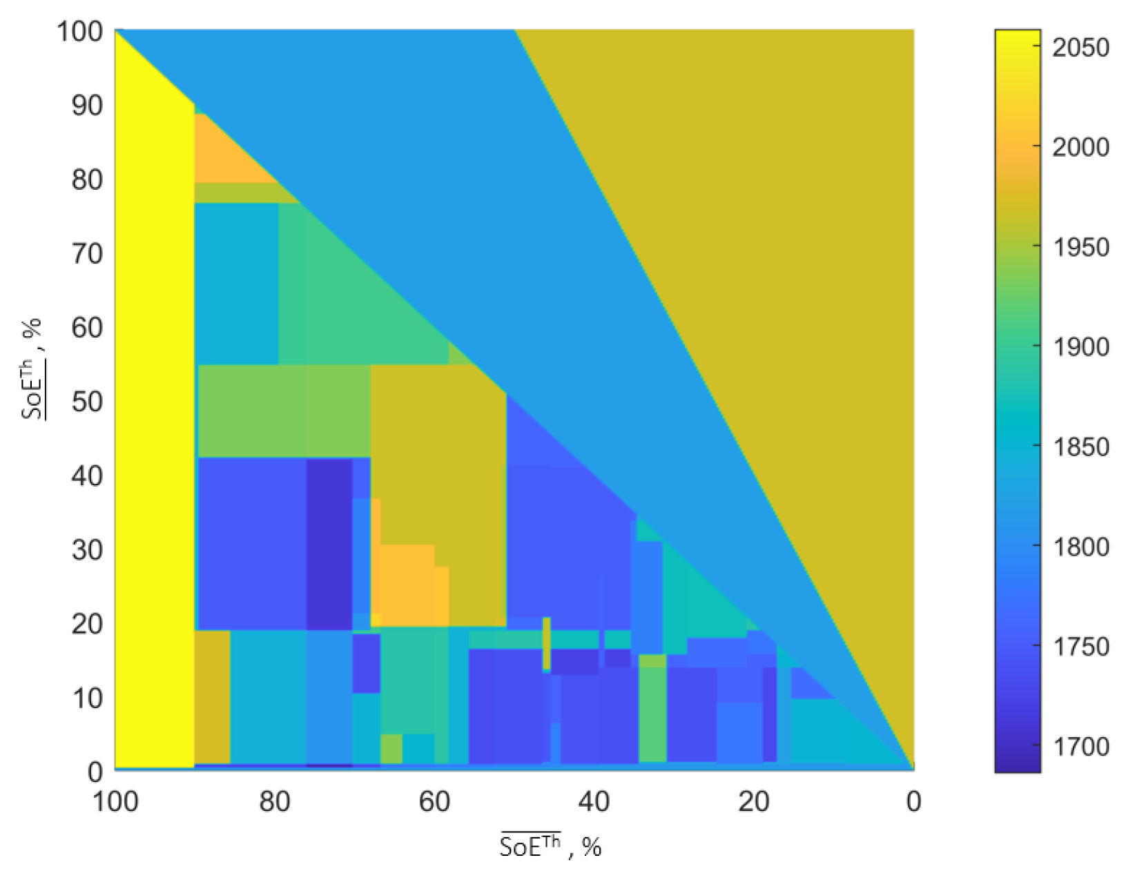
Figure 6 shows an example of the cost function for a single operating day, assuming that the SoE thresholds are constant throughout the day.

The search space is divided, as expected, into three parts: the top-right part of the search space corresponds to the SP strategy, the central part to the LF, and the bottom left to the CC. The first two strategies are not affected by the value of the SoE thresholds, and therefore, are associated with flat surfaces. The CC strategy is instead affected by the combination of thresholds considered, and it is possible to see that the cost function is multimodal, and it is formed by a set of flat subspaces. When the number of intra-day intervals increases, the objective function space becomes more complex, but it preserves its basic features.

This cost surface justifies the use of Evolutionary Algorithm for the optimization of the TRBH. In fact, they can handle multimodal function thanks to the use of a population of candidate solutions; moreover, they do not rely on gradient information, thus they are not negatively affected by plateaus.

When tackling the optimal tuning problem, the population size has been set to 25 individuals and 100 iterations were completed, performing 2500 objective function calls. Due to the stochastic nature of the algorithm, 20 independent trials were always performed.

SNO was firstly compared with other algorithms in this problem. The other tested algorithms are the Differential Evolutionary (DE), the Biogeography Based Optimization (BBO), the Stud-Genetic Algorithm (SGA), and the Particle Swarm Optimization (PSO).

For each algorithm, the mean values obtained in each of the 28 tested scenarios are compared. Figure 7 shows the results of this comparison: for each algorithm the number of losses are counted, i.e., the number of times in which its average value is higher than the minimum one achieved. It is important to note that in most of the cases, several algorithms achieve the same results, meaning that this is most likely to be the global optimum.

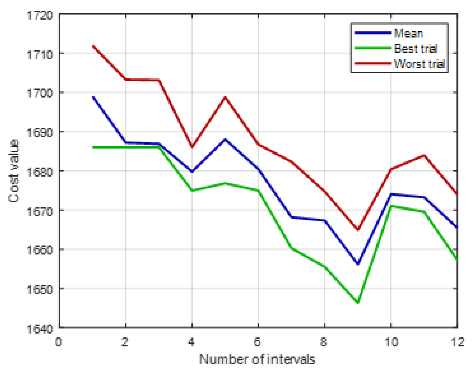
A preliminary analysis was carried out on the impact of the number of intra-day intervals on the TRBH performance. Figure 8 shows the results of this test on the same day considered in Figure 8. For each set of parameters, the graph shows the mean, best, and worst fitness of the optimal heuristic tuning over the 20 independent optimization trials. The performance of the optimal heuristic tuning tends to increase with the number of intra-day windows, which guarantee a more flexible dispatch strategy structure. The irregularities in the trend are due to how the hours of the day are clustered differently according to the spacing of the intra-day windows: some clustering configurations will allow the switch from one strategy to another at more appropriate hours of the day. The dispersion of the optimization trials is due to the stochastic nature of all the Evolutionary Algorithms; nevertheless, the mean performance is, on average, only about 0.5% from the best solution.

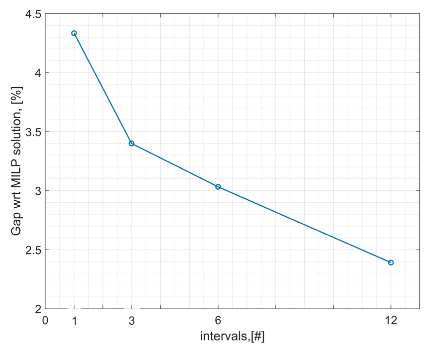
The effect of the number of intra-day windows considered in the TRBH structure is confirmed by the performance of the TRBH over all the considered sample days. Results are measured in terms of average percentage cost increase compared to the MILP solution (Figure 9). Only a selected set of intra-day windows numbers (1, 3, 6, 12 intervals) are plotted so that each solution with a higher number of intervals is contained in the coarser configurations, avoiding the effect of changes in the position of the interfaces between hours of the day that may influence the trend due to the coarse time step used in the simulation. From Figure 9, it is evident how increasing the number of intraday intervals is beneficial to reduce the gap with respect to the MILP solution.

5.3. Dispatch Results Comparison

The performance of the TRBH with 12 intra-day windows (TRBH12) can finally be compared with the alternative scheduling strategies, including direct scheduling optimization with the SNO algorithm, and the traditional LF and CC heuristic strategies. The comparison of the TRBH with LF and CC is particularly interesting, as the two are special instances of the TRBH structure. Performances are characterized in terms of percentage cost increase with respect to the MILP solution (referred to as gap), constituting, as mentioned, the objective function lower bound.

TRBH12 significantly outperforms all other methods, with an average distance from the MILP solution of only 2.39%. Resorting to the SNO algorithm to directly optimize the scheduling decisions appears to be less effective, as a large number of variables and the complexity of the scheduling problem solution-space is not well suited for this optimization methodology. Nevertheless, the SNO average distance from global optimality is only 5.31%, although this value is expected, for more complex system architectures, its competitiveness would quickly reduce. LF and CC perform significantly worse than the two optimized methods, although they attain an acceptable performance especially during the days that are well suited to their management philosophy (

Table 1. Average gap attained by each method over all simulated days of operation. The 10th and 90th percentiles are also shown, to give an idea of the reliability of the scheduling approach in operating days with different characteristics.

	Strategy
	TRBH	SNO	LF	CC
10th perc.	1.43%	3.72%	10.79%	6.71 %
Average	2.39%	5.31%	12.45%	10.46%
90th perc.	3.41%	6.25%	13.99%	17.21%

).

Figure 10 shows the gap for the four scheduling approaches in the four days corresponding to the best performance of each method. As expected, the best performance of the LF strategy corresponds to a particularly bad performance of the CC strategy and vice versa, since the two represent opposite approaches to the battery management strategy. It is also interesting to notice that neither of the two dominates the other (although LF is, on average, performing better), and the suitability of one strategy with respect to the other depends on the specific profiles of demand and RES production in the day under analysis.

The flexibility of the TRBH structure on the other hand allows switching from one to the other throughout the day, resulting in a dramatically improved overall performance despite starting from the same logical blocks (with the addition of the SoC preservation option).

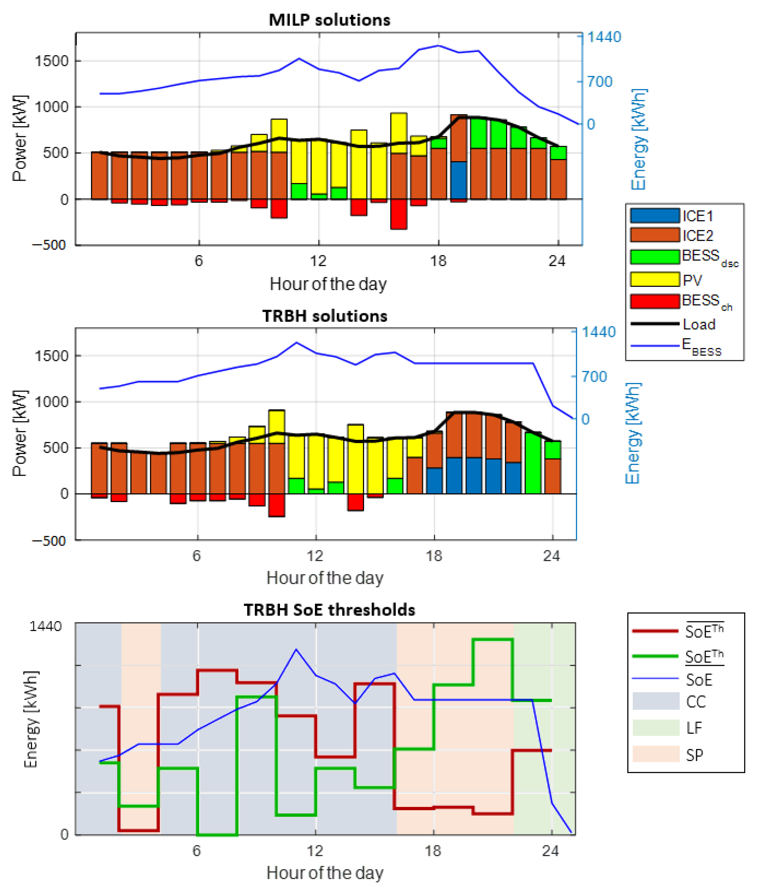
Finally, Figure 11 shows a comparison of the detailed dispatch profiles yielded by the MILP formulation and by the TRBH12, on the day during which the performance difference between the methods is minimal. The two methods come to very similar scheduling decisions, and the TRBH12 manages to mimic the behavior of the MILP solution by adjusting the SoE thresholds during the day (Figure 11-bottom), combining the available operating modes.

Overall, the TRBH has proven to be an effective dispatch strategy. It consistently achieves an improved performance with respect to both standard rule-based logics (LF and CC) because the ability to switch among different operating modes allows the TRBH to adapt to the external operating conditions (i.e., load and RES profiles).

Furthermore, the heuristic strategies implemented inside the TRBH reduce the degrees of freedom of the optimization problem with respect to the pure EA approach, leading to an improved performance. In fact, incorporating an already effective response dispatch structure, which can be properly adjusted acting on a limited set of parameters, greatly simplifies the optimization problem with respect to a fully unconstrained approach.

In virtue of the highlighted advantages, the TRBH is able to closely approach the MILP objective function, which constitutes the absolute performance lower bound since the uncertainty effect has been neglected.

6. Conclusions

This paper presents a new approach to the optimal scheduling of hybrid off-grid microgrids, consisting in the predictive tuning of a Tunable Rule-Based Heuristic (TRBH) dispatch logic based on the forecasts of demand and RES generation potential. The parameters defining the TRBH behavior are optimally adjusted using Evolutionary Optimization Algorithms (EA), and the resulting performance is compared with alternative scheduling approaches, including conventional rule-based logics and MILP optimization. The developed algorithm:

• Significantly outperforms the standard rule-based logics LF and CC that constitute its building blocks by identifying the optimal combination of operating modes during different hours of the day that can minimize operating costs;
• Outperforms the direct use of EAs to tackle the optimal scheduling problem, showing how a dispatch strategy structure based on physical considerations can reduce the number of optimization variables and guide the EA towards better decisions
• Shows comparable results with respect to a perfect foresight MILP, defining the global optimum for the daily operating cost.

Moreover, with respect to the EA and MILP approaches, TRBH can be directly implemented in the microgrid PLC without any need for a re-dispatching layer that manages forecast errors.

Future work will focus on a deeper assessment of the TRBH potential adoption in real-life systems, extending the comparison with other predictive approaches by explicitly addressing the uncertainty of forecasts and including the effect of the re-dispatching layer in the evaluation. The training procedure will be pursued with a stochastic approach, defining the fitness of the candidate over a family of scenarios, representative of the variability of the uncertain parameters.