
Thermal Analyses of Reactor under High-Power and High-Frequency Square Wave Voltage Based on Improved Thermal Network Model

Abstract
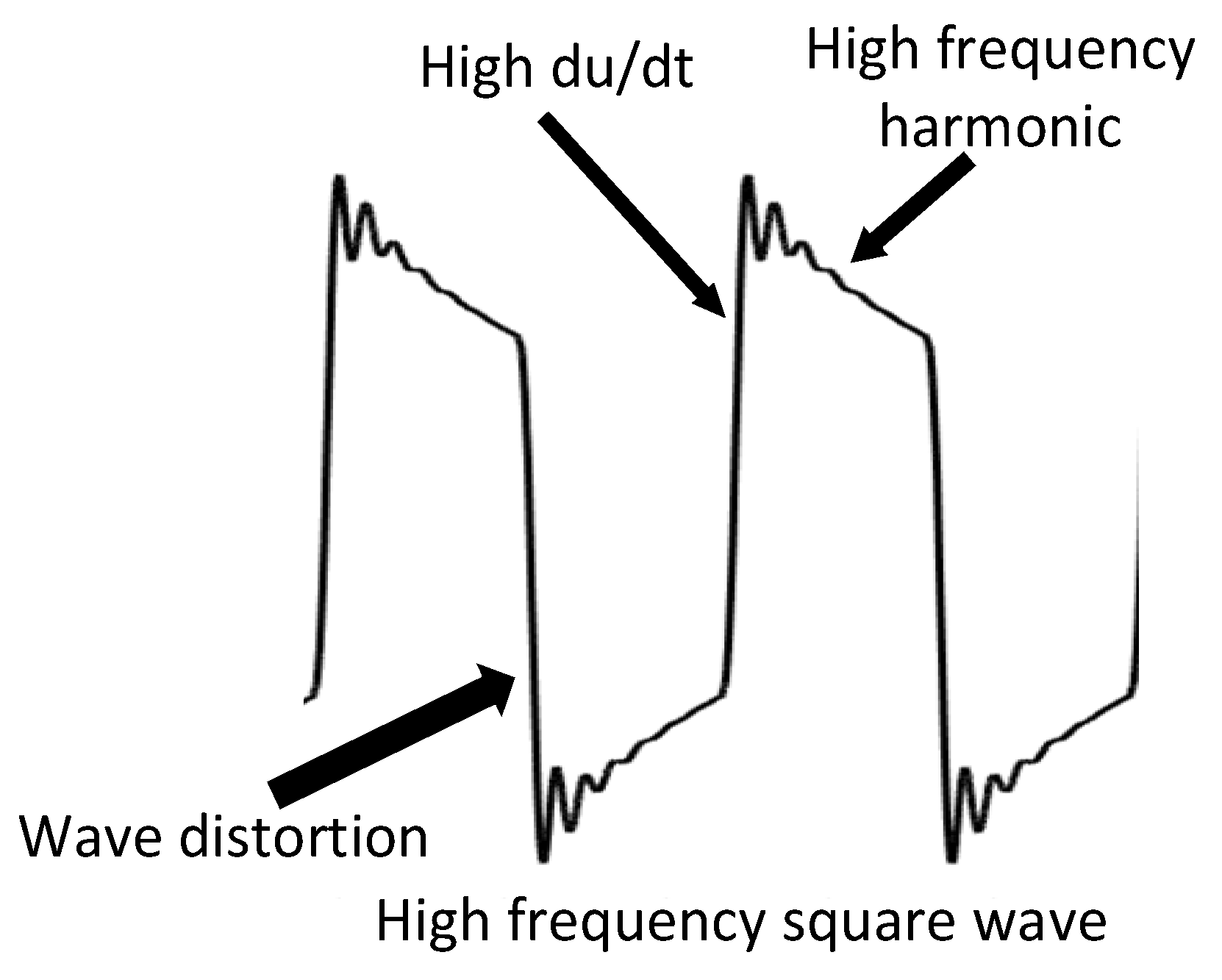
:1. Introduction
2. The Thermal Network Model of the Reactor
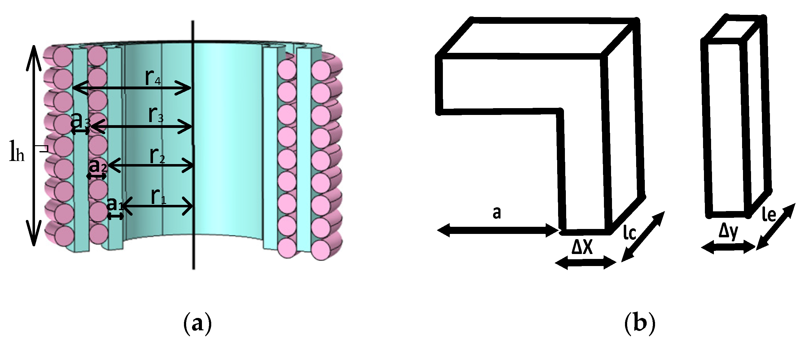
2.1. Conventional Temperature Model
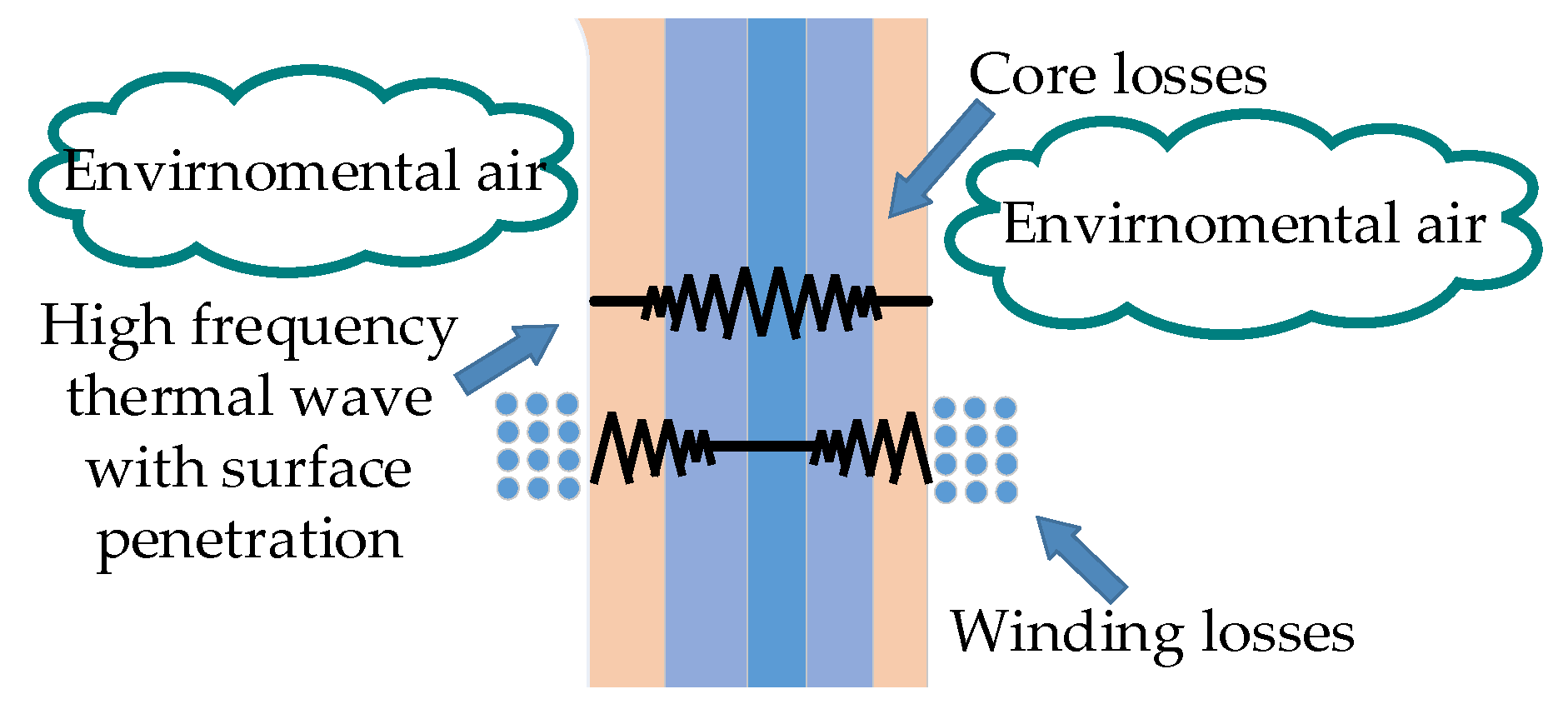
2.2. Heat Transfer Analysis
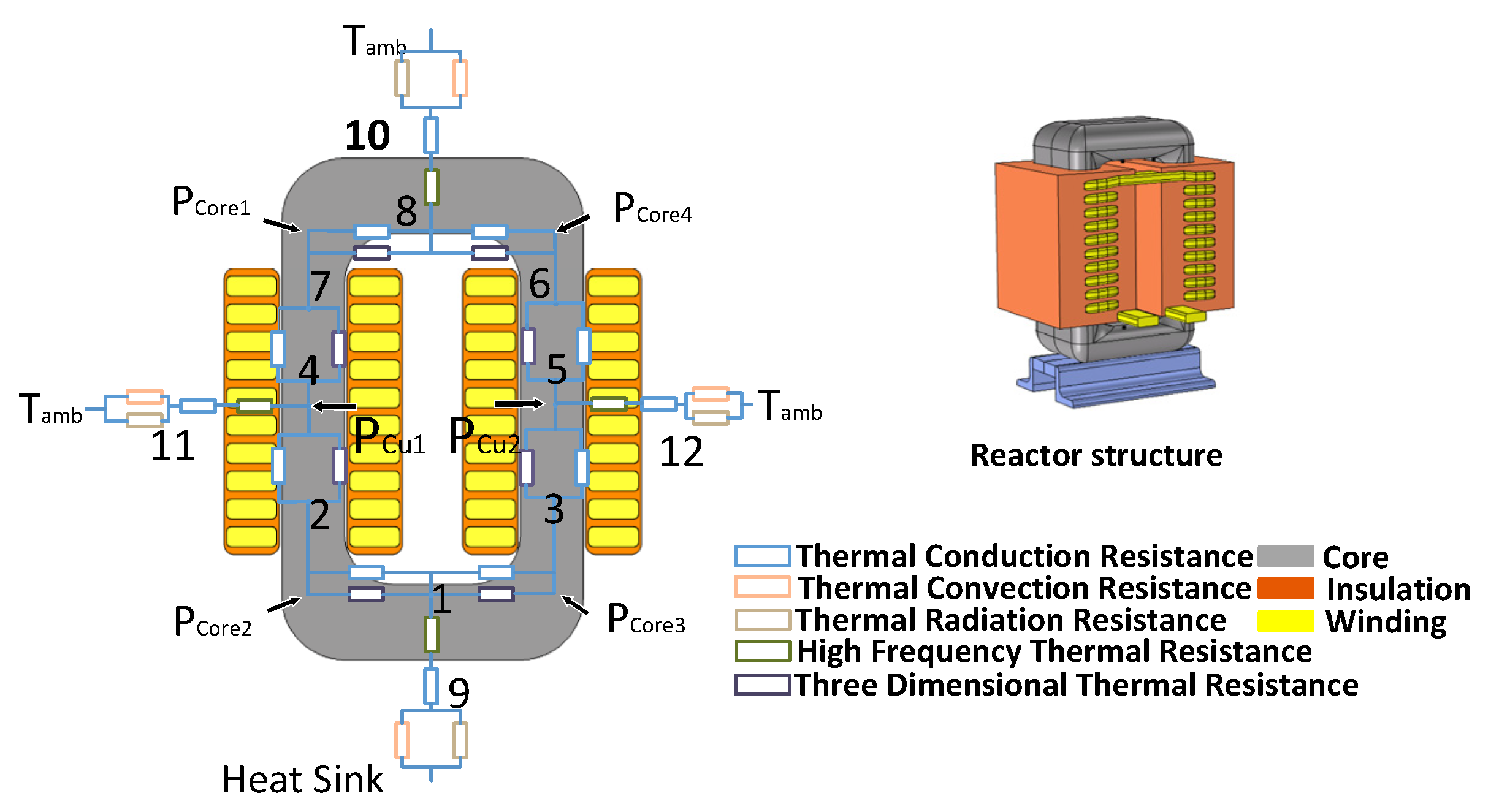
2.3. The Reactor Thermal Network Model and Temperature Calculation
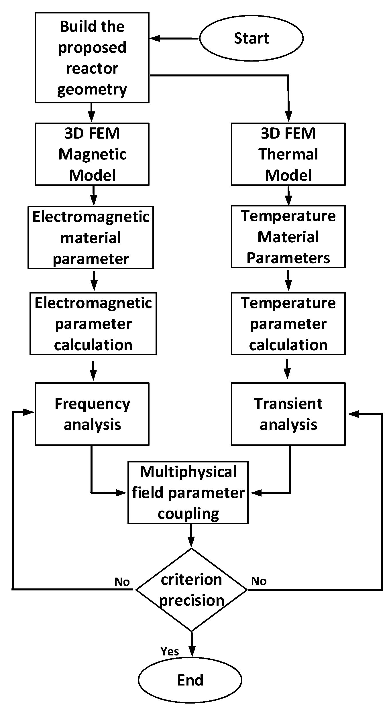
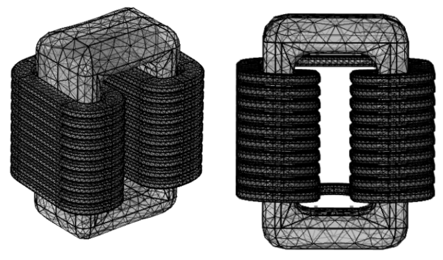
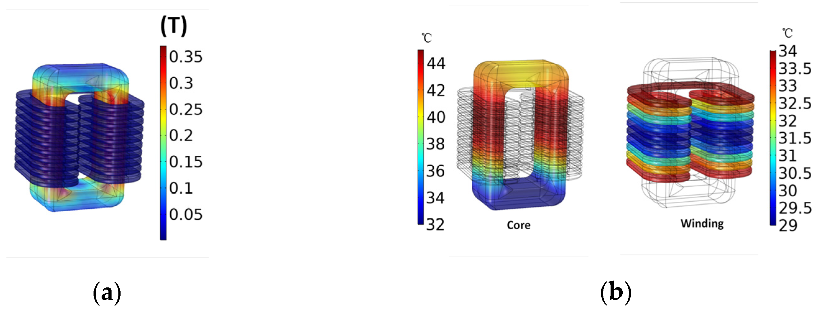
3. Finite Element Simulation
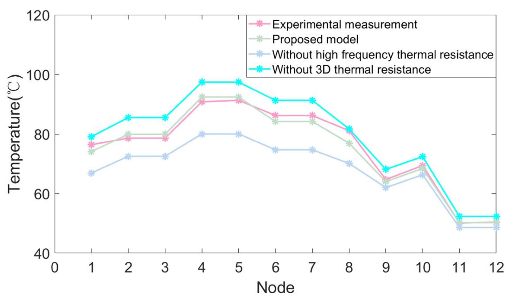
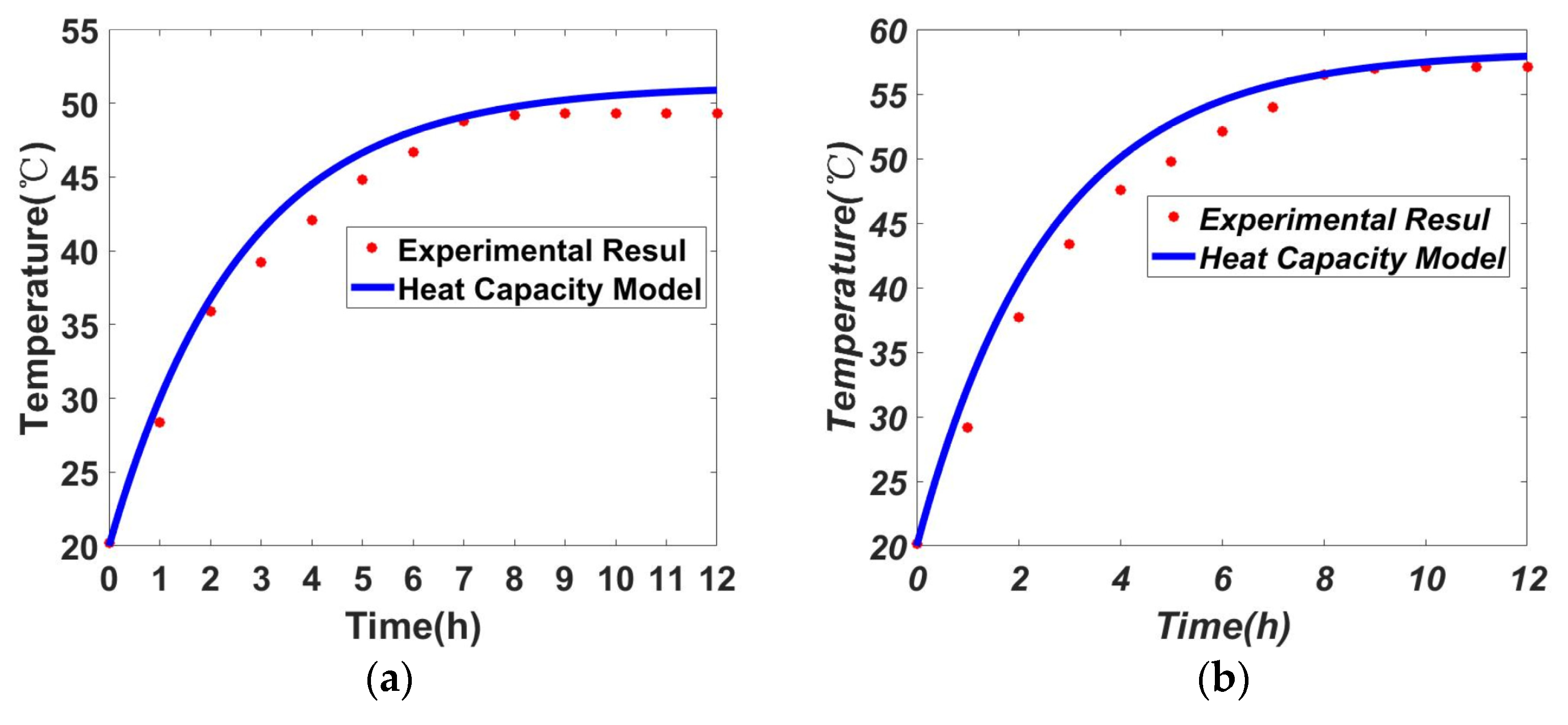
4. Experimental Verification
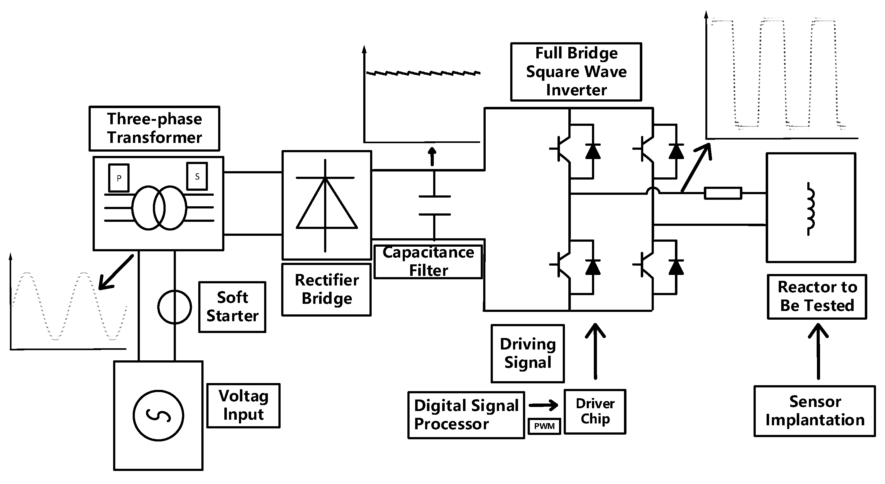
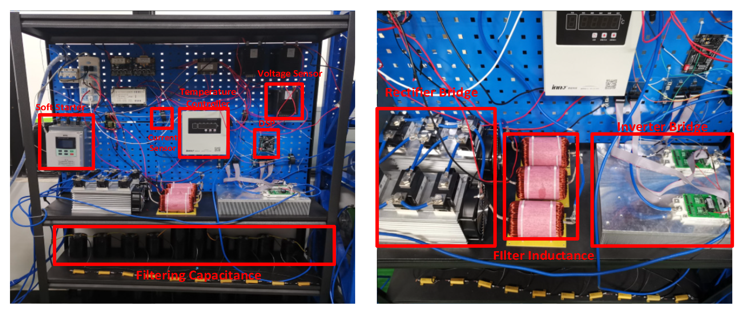
4.1. Construction of Experimental Platform
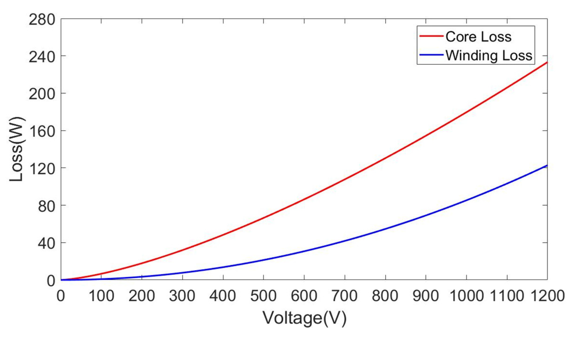
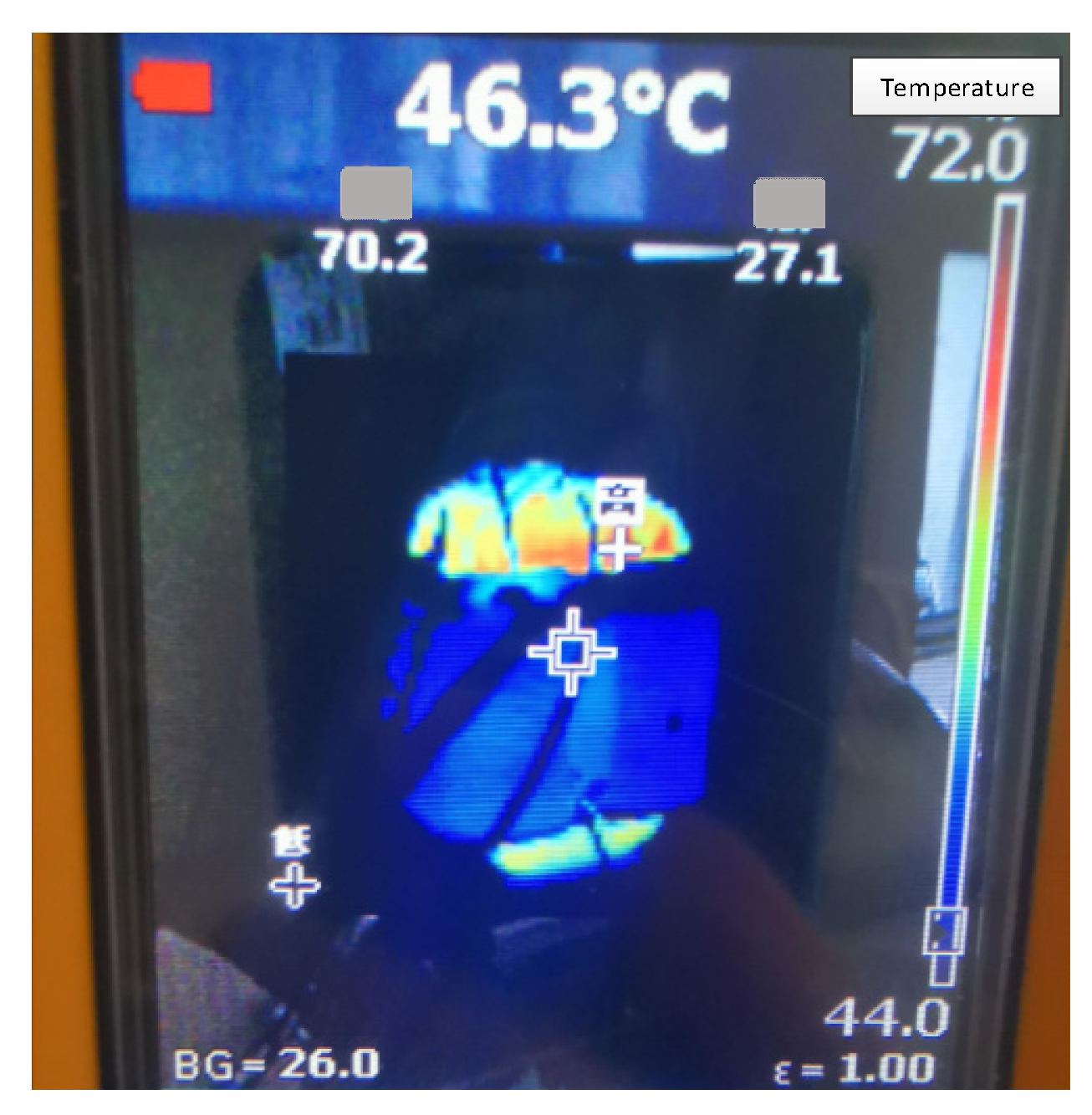
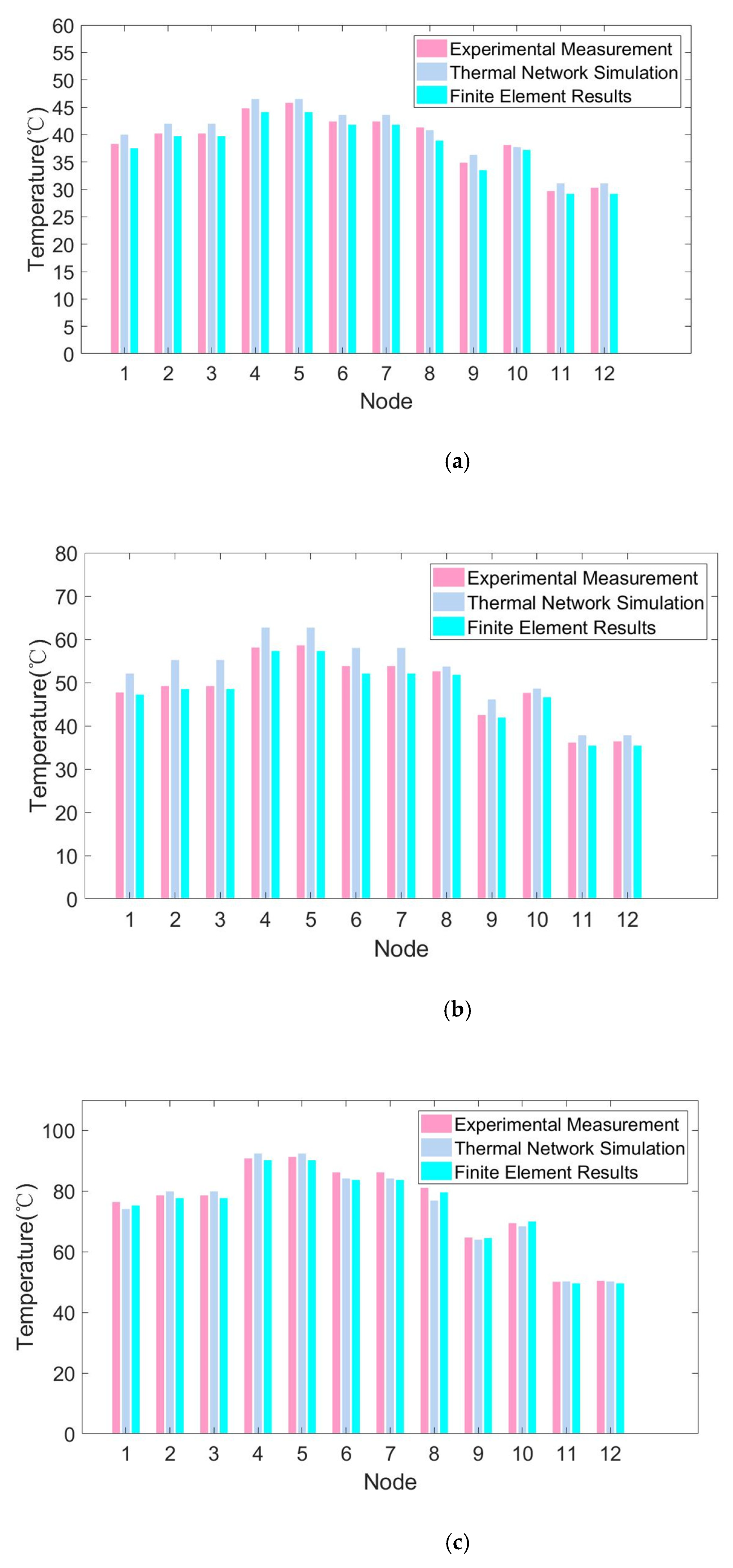
4.2. Experimental Analysis
5. Conclusions
Author Contributions
Funding
Informed Consent Statement
Conflicts of Interest
References
- Nasser, H.; Asma, A. Voltage Stability of Power Systems with Renewable-Energy Inverter-Based Generators: A Review. Electronics 2021, 10, 115. [Google Scholar]
- Li, C.; Gole, A.M.; Zhao, C. A Fast DC Fault Detection Method Using DC Reactor Voltages in HVDC Grids. IEEE Trans. Power Deliv. 2018, 33, 2254–2264. [Google Scholar] [CrossRef]
- Liu, G.H.; Zhang, Y.N.; Chen, Z.L.; Jia, H.P. PMSM DTC predictive control system using SVPWM based on the subdivision of space voltage vectors. In Proceedings of the 2009 IEEE 6th International Power Electronics and Motion Control Conference, Wuhan, China, 17–20 May 2009; pp. 1818–1821. [Google Scholar]
- Li, H.Y.; He, M.; Huang, L. Correlation between the Generation of Acidic Products and the Thermal Aging of Oil-paper Insulation of the UHV Transformer. High Volt. Eng. 2015, 6, 1959–1964. [Google Scholar]
- Ghahfarokhi, P.S.; Kallaste, A.; Vaimann, T. Steady-State Thermal Model of a Synchronous Reluctance Motor. In Proceedings of the 2018 IEEE 59th International Scientific Conference on Power and Electrical Engineering of Riga Technical University (RTUCON), Riga, Latvia, 12–14 November 2018; pp. 1–5. [Google Scholar]
- Guo, Y.G.; Zhu, J.G.; Wu, W. Thermal analysis of soft magnetic composite motors using a hybrid model with distributed heat sources. IEEE Trans. Magn. 2005, 41, 2124–2128. [Google Scholar]
- Santisteban, A.; Piquero, A.; Ortiz, F.; Delgado, F.; Ortiz, A. Thermal Modelling of a Power Transformer Disc Type Winding Immersed in Mineral and Ester-Based Oils Using Network Models and CFD. IEEE Access 2019, 7, 174651–174661. [Google Scholar] [CrossRef]
- Liu, C.; Ruan, J.J.; Liang, S.Y. Improvement of Transformer Air Duct with Thermal-fluid Coupled Field Simulation by FEM. Water Resour. Power 2016, 34, 195–198. [Google Scholar]
- Górecki, K.; Detka, K.; Górski, K. The Nonlinear Compact Thermal Model of the Pulse Transformer. In Proceedings of the 25th International Workshop on Thermal Investigations of ICs and Systems (THERMINIC), Lecco, Italy, 25–27 September 2019; pp. 1–4. [Google Scholar]
- Sayani, M.P.; Skutt, G.R.; Venkatraman, P.S. Electrical and thermal performance of PWB transformers. In Proceedings of the APEC ’91: Sixth Annual Applied Power Electronics Conference and Exhibition, Dallas, TX, USA, 10–15 March 1991; pp. 533–542. [Google Scholar]
- Kyaw, P.A.; Delhommais, M.; Qiu, C. Thermal Modeling of Inductor and Transformer Windings Including Litz Wire. IEEE Trans. Power Electron. 2020, 35, 867–881. [Google Scholar] [CrossRef]
- Wang, L.; Zhou, L.; Yuan, S. Improved Dynamic Thermal Model With Pre-Physical Modeling for Transformers in ONAN Cooling Mode. IEEE Trans. Power Deliv. 2019, 34, 1442–1450. [Google Scholar] [CrossRef]
- Jaritz, M.; Biela, J. Analytical model for the thermal resistance of windings consisting of solid or litz wire. In Proceedings of the 2013 15th European Conference on Power Electronics and Applications (EPE), Lille, France, 2–6 September 2013; pp. 1–10. [Google Scholar]
- Eslamian, M.; Ahidi, V.; Eslamian, B.A. Thermal analysis of cast-resin dry-type transformers. Energy Convers. 2011, 52, 2479–2488. [Google Scholar] [CrossRef]
- Marian, K.K. High-Frequency Magnetic Components, 2nd ed.; Wiley: Hoboken, NJ, USA, 2013; pp. 293–296. [Google Scholar]
- Yang, S.M.; Tao, W.Q. Heat Transfer, 4th ed.; Higher Education Press: Beijing, China, 2006; pp. 4–12. [Google Scholar]
- Jain, A.; Jones, R.E.; Chatterjee, R.; Pozder, S. Analytical and Numerical Modeling of the Thermal Performance of Three-Dimensional Integrated Circuits. IEEE Trans. Compon. Packag. Technol. 2010, 33, 56–63. [Google Scholar] [CrossRef]
- Bergman, T.L.; Lavine, A.S.; Incropera, F.P.; Dewitt, D.P. Fundamentals of Mass and Heat Transfer, 7th ed.; Wiley: Hoboken, NJ, USA, 2011; pp. 46–78. [Google Scholar]
- Shafaei, R.; Ordonez, M.; Saket, M.A. Three-Dimensional Frequency-Dependent Thermal Model for Planar Transformers in LLC Resonant Converters. IEEE Trans. Power Electron. 2019, 34, 4641–4655. [Google Scholar] [CrossRef]
- D’Esposito, R.; Balanethiram, S.; Battaglia, J.; Frégonèse, S.; Zimmer, T. Thermal Penetration Depth Analysis and Impact of the BEOL Metals on the Thermal Impedance of SiGe HBTs. IEEE Electron Device Lett. 2017, 38, 1457–1460. [Google Scholar] [CrossRef] [Green Version]
- Chen, J.; Ma, J.; Fang, Y. An Improved Steinmetz Premagnetization Graph (SPG) Applied in High Magnetic Field. In Proceedings of the 22nd International Conference on Electrical Machines and Systems (ICEMS), Harbin, China, 11–14 August 2019; pp. 1–5. [Google Scholar]
- Whitman, D.; Kazimierczuk, M.K. An Analytical Correction to Dowell’s Equation for Inductor and Transformer Winding Losses Using Cylindrical Coordinates. IEEE Trans. Power Electron. 2019, 34, 10425–10432. [Google Scholar] [CrossRef]


| Reactor Regulation | Magnetic Core | Winding | Insulation |
| L20A2M-0PH | Ni-Zn Ferrite | Copper | Polyester Film |
| Rated Current | Rated Temperature | Frequency | Inductance |
| 20 A | 100 °C | 0–50 kHz | 2 mH |
| Nodes | ||
|---|---|---|
| 1: Core bottom column | 2: Core bottom left corner | 3: Core bottom right corner |
| 4: Core left column | 5: Core right column | 6: Core top right corner |
| 7: Core top left corner | 8: Core top column | 9: Core bottom surface |
| 10: Core top surface | 11: Left winding surface | 12: Right winding surface |
| Node | xi | yi | Node | xi | yi |
|---|---|---|---|---|---|
| 1 | 0.2224 | 0.1160 | 5 | 0.2851 | 0.1854 |
| 2 | 0.2356 | 0.1540 | 6 | 0.2558 | 0.1586 |
| 3 | 0.2356 | 0.1540 | 7 | 0.2558 | 0.1586 |
| 4 | 0.2851 | 0.1854 | 8 | 0.2312 | 0.1310 |
| Item | V | T0 | ||||
| Value | 550 | 20,000 | 5.998 × 10⁷ | 385 | 8940 | 293.15 |
| Item | μc | |||||
| Value | 526 | 800 | 0.004 | 8600 | 1393 | 1 |
| Item | ||||||
| Value | 152 | 400 | 0.8 | 386 | 0.27 |
Publisher’s Note: MDPI stays neutral with regard to jurisdictional claims in published maps and institutional affiliations. |
© 2021 by the authors. Licensee MDPI, Basel, Switzerland. This article is an open access article distributed under the terms and conditions of the Creative Commons Attribution (CC BY) license (https://creativecommons.org/licenses/by/4.0/).
Share and Cite
Shen, L.; Xie, F.; Xiao, W.; Ji, H.; Zhang, B. Thermal Analyses of Reactor under High-Power and High-Frequency Square Wave Voltage Based on Improved Thermal Network Model. Electronics 2021, 10, 1342. https://0-doi-org.brum.beds.ac.uk/10.3390/electronics10111342
Shen L, Xie F, Xiao W, Ji H, Zhang B. Thermal Analyses of Reactor under High-Power and High-Frequency Square Wave Voltage Based on Improved Thermal Network Model. Electronics. 2021; 10(11):1342. https://0-doi-org.brum.beds.ac.uk/10.3390/electronics10111342
Chicago/Turabian StyleShen, Li, Fan Xie, Wenxun Xiao, Huayu Ji, and Bo Zhang. 2021. "Thermal Analyses of Reactor under High-Power and High-Frequency Square Wave Voltage Based on Improved Thermal Network Model" Electronics 10, no. 11: 1342. https://0-doi-org.brum.beds.ac.uk/10.3390/electronics10111342