Simplified Swarm Optimization for the Heterogeneous Fleet Vehicle Routing Problem with Time-Varying Continuous Speed Function

Abstract

Transportation planning has been established as a key topic in the literature and practices of social production, especially in urban contexts. To consider traffic environment factors, more and more researchers are taking time-varying factors into account when scheduling their logistic activities. The time-dependent vehicle routing problem (TDVRP) is an extension of the classical Vehicle Routing Problem with Time Windows (VRPTW) by determining a set of optimal routes serving a set of customers within specific time windows. However, few of them use the continuous speed function to express the time-varying. In practice, many vehicle routing problems are addressed by a fleet of heterogeneous vehicles with different capacities and travel costs including fix costs and variable costs. In this study, a Heterogeneous Fleet Vehicle Routing Problem (HFPRP) Time-Varying Continuous Speed Function has been proposed. The objective is to minimize distribution costs, which contained fixed costs of acquiring and variable fuel costs. To address this problem, our research developed a mathematical model and proposed a Simplified Swarm Optimization (SSO) heuristic for HFVRP with Time-Varying Continuous Speed Function.

1. Introduction

Throughout recent decades, transportation planning has been established as a key topic in the literature and practices of social production. Especially in urban contexts, due to industrial strategies, urbanization, city design and unforeseen accidents, weather conditions, traffic congestion, logisticians and citizens face many challenges related to delivery delays [1]. The traffic environment is dynamically changing, which increases the complexity of the problem, the most obvious one being time-varying travel time. Travel velocity is significantly reduced during peak hours. Therefore, to achieve socio-economic and environmental sustainability in city transportation, a major intervention on time-varying congestion is needed.

Problems related to the distribution of goods between the warehouse and the final customer are generally considered as the vehicle routing problem (VRP). The vehicle routing problem was first raised by Dantzig and Ramser [2]. Clarke and Wright [3] added more practical restrictions for the problems, in which the delivery of goods to each customer should have occurred in the bound. Such a problem model is called the Vehicle Routing Problem with Time Windows (VRPTW). The actual distribution process is much more complex, such as travel speeds on the road varying substantially during peak and off-peak hours in the urban areas. Consequently, Malandraki and Daskin [4] first took the existence of diversified conditions of traffic at different times of the day. They discussed the Time-Dependent Vehicle Routing Problem (TDVRP) where the travel time was based on “a step function distribution”. Unfortunately, this model does not satisfy the First-In-First-Out (FIFO) property which ensures that if a vehicle leaves a node i for a node j at a given time, any other vehicle leaving a node i for a node j at an earlier time will arrive earlier at node j. Without the “FIFO” property, that is, a vehicle can depart later than another vehicle and arrive earlier at its destination, even if the same path is followed by the two vehicles. This situation is contrary to reality, but it happens in the assumptions of the model, for example, if one vehicle waits just a little before departing to catch a faster travel time associated with the next interval.

Previous studies tend to use different travel link times of node i and node j to guarantee the FIFO property. Ichoua et al. [5] presented a model based on time-dependent travel speeds that they proved to be better at modeling time-dependency, and the FIFO assumption is not necessarily satisfied either. The idea of time-varying speed is adopted in our problem as well. At the same time, the time-varying continuous speed model is closer to the actual distribution situation, the speed of vehicles changes smoothly, rather than a step-change at a certain moment [6,7].

Apart from the Time-Dependent VRPs, another variant of the VRPs is named the Heterogeneous Fleet Vehicle Routing Problem (HFVRP), where a heterogeneous fleet of vehicles is used for the distribution activities; see Baldacci et al. [8]. The HFVRP with a limited number of vehicles proposed by Taillard [9] involves optimizing the vehicle routes with the available fixed fleet. The idea is not only to consider the routing of the vehicles, but also the fleet composition. Relating to the type of costs (fixed and variable) to be minimized, two different objective functions have been considered.

In the case of just-in-time (JIT) production and urban logistics distribution, time-varying speed, time windows, and heterogeneous fleet settings naturally occur and are therefore more in line with the actual distribution situation. Logistics need to find a balance between costs and quality of service. This route construction problem has been encountered by the authors in several contexts: e.g., cold chain logistics [10], fresh logistics [11], milk run [12], automated guided vehicle (AGV) systems [13], freight distribution [14], JIT production [15], B2C e-commerce [16], inter-vehicle communication [17], vaccine distribution [18], and so on. Nonetheless, there are few cases involving optimization of vehicle type selection and route distribution under the minimizing of total cost based on a continuous time-varying speed model which are closer to the actual distribution situation.

Solving VRP is computationally expensive as it is categorized as NP-Hard; see Lenstra and Kan [19]. Metaheuristics approaches are necessary to solve this problem within considerable computational time. Compared to the classical heuristic, metaheuristics carry out a more thorough search of the solution space. Thus, they are notably capable of consistently producing high-quality solutions, despite the greater computational time than early heuristics; see Cordeau et al. [20]. They have been successfully applied for different combinatorial optimization problems. However, in the scientific literature, almost all existing memetic algorithms for solving different VRP variants follow the framework of genetic algorithms (GA) [21,22,23] or the Particle Swarm Optimization algorithm (PSO) [24,25] and very rarely, the framework of Simplified Swarm Optimization algorithms.

As one metaheuristic methodology, the Simplified Swarm Optimization (SSO) is often used to address both discrete and continuous optimization problems (Yeh [26]; Yeh [27]; Yeh and Chuang [28]). SSO has some attractive advantages such as its ability to deal with non-linear models, chaotic and noisy data, and many constraints.

The rest of this paper is organized as follows. In Section 2, the literature review is presented, and the problem statement is described in Section 3. Simplified Swarm Optimization is presented in Section 4. Details of the computational result and analysis about the problem are presented in Section 5. Section 6 draws conclusions and possible future research.

2. Literature Review

Vehicle Routing Problems (VRP) are essential elements of distribution systems for delivering goods and services. The effective management of these vehicles could improve customers’ experience of delivery and minimize the total routing costs. Due to the wide application of logistics distribution scenarios, there is more and more research on VRPs, so there are a lot of different objective types and limit types of VRPs.

Hence, we have briefly reviewed two different types of VRPs: (1) those that model Time-Dependent travel time VRP with a speed model, (2) and the Heterogeneous Fleet VRP is introduced. Time Dependent VRP (TDVRP) with Time-Varying Speeds and Heterogeneous Fixed Fleet VRP (HFFVRP) in Section 2.1 and Section 2.2, respectively.

2.1. Time Dependent Vehicle Routing Problem with Time-Varying Speeds

As the Time Dependent VRP (TDVRP) was proposed, since its assumption was more in line with the realistic world, the TDVRP has attracted the attention of many researchers. However, literature on the speed model remains scarce. The pioneering work has been done by Malandraki and Daskin [4] and Malandraki and Dial [29]. In these papers, mixed-integer linear programs (MILP) and several heuristics to solve the problem are proposed. However, these models may potentially violate the First-In-First-Out (FIFO) property, which implies that for every arc, a later departure time results in a later (or equal) arrival time.

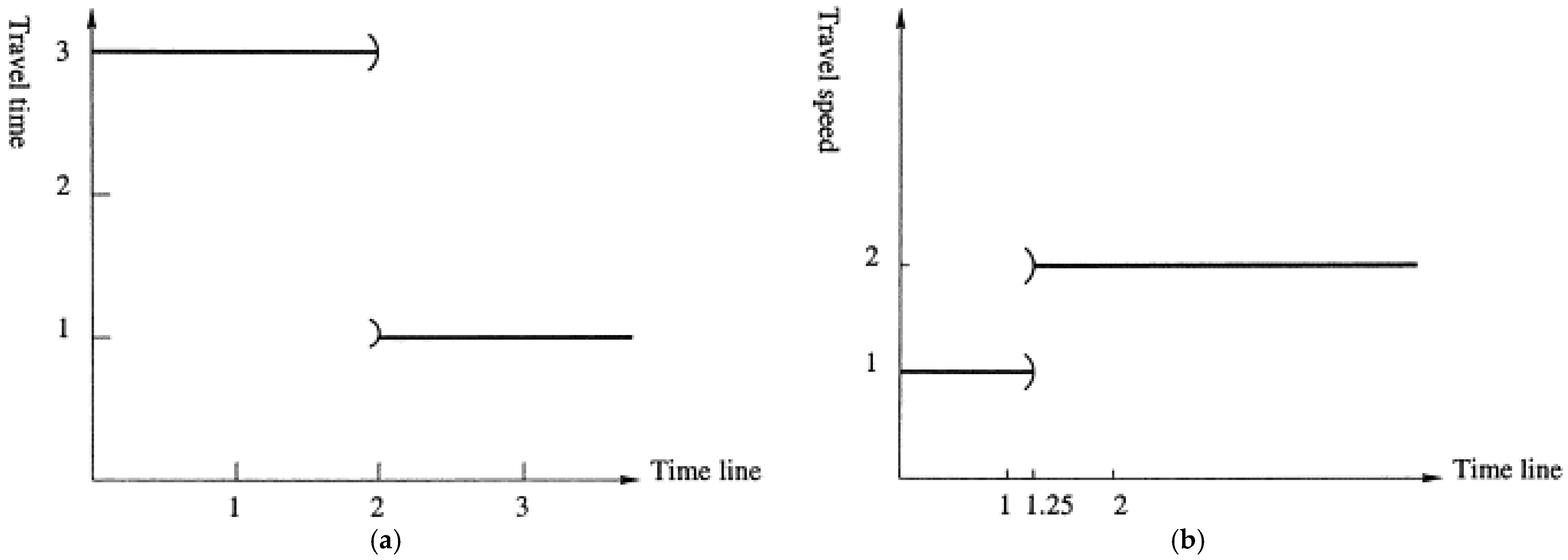
As opposed to Malandraki and Daskin [4], Ichoua, Gendreau, and Potvin [5] proposed an alternative approach model; a stepwise speed function was proposed, resulting in a piecewise linear travel time function, like the one illustrated in Figure 1a, where the day is divided into several time periods and a speed is associated with each period. For a given arc, a stepwise speed function can easily be translated into a corresponding piecewise linear travel time function, as shown in Figure 1b.

This new travel time model satisfies the FIFO principle since a vehicle can only arrive later at the destination if it departs later. The time-dependent speed model is commonly adopted in later publications on VRP variants with time-dependent travel times

Çimen and Soysal [30] addressed a TDVRP with stochastic vehicle speeds and environmental concerns and formulated the problem as a Markovian Decision Process. Soysal and Çimen [31] also proposed a GTDVRP that accounts for transportation emissions, and the problem has been formulated and solved using the Dynamic Programming approach. Sun et al. [32] introduced a time-dependent capacitated profitable tour problem with the object to maximize the profit and developed a tailored labeling algorithm to find the optimal tour. Wang, Assogba, Fan, Xu, Liu, and Wang [14] presented a bi-objective model which focused on freight distribution to minimize total carbon emission and operating cost. Adriano, Montez, Novaes, and Wangham [12] also proposed a dynamic model to simulate the milk-run tours with time windows, using the auxiliary vehicle to deal with traffic jams. Liu et al. [33] proposed TDVRPTW to minimize the sum of the fixed costs of the vehicle used, as well as the costs of drivers, fuel consumption, and carbon emissions. Pan et al. [34] studied the duration-minimizing time-dependent vehicle routing problem with time windows (DM-TDVRPTW), where time-dependent travel times represent different levels of road congestion throughout the day. Pan et al. [35] also proposed a multi-trip time-dependent vehicle routing problem with time windows (MT-TDVRPTW) and formulated the time-dependent ready time function and duration function for any segment of consecutive nodes as piecewise linear functions. Gmira et al. [36] proposed a time-dependent vehicle routing problem with time windows in which travel speeds are associated with road segments in the road network.

Few papers use the time-varying speed of continuous function. Xiao and Konak [37] defined GVRSP which considers heterogeneous vehicles and time-varying traffic congestion where the speed of smooth period is variable. Huang et al. [38] proposed the time-varying speed of the linear continuous function model, but without detailed specification, and their research only studied two types of vehicles with a fixed cost. Xu, Elomri, Pokharel, and Mutlu [21] extended the period-based speed pattern to be a time-varying speed pattern. The approximate corresponding function denoting the relationship between the departure time t and the vehicle speed $\mathrm{v}\left(t\right)$ can be characterized by the trigonometric function. Fan, Zhang, Tian, Lv, and Fan [23] continued the assumption in which speed is a trigonometric function of the departure time and applied it in time-dependent multi-depot GVRP. We should still express the time-varying speed as a linear continuous function, without loss of generality, and amplify the speed transformation time to illustrate the time-varying speed of continuous function.

2.2. Heterogeneous Fixed Fleet Vehicle Routing Problem

In practice, many vehicle routing problems are addressed by a non-homogeneous vehicle fleet where vehicles of different capacities are used. Heterogeneous fleets VRPs (HFVRPs) are consider a limited or an unlimited fleet of capacitated vehicles, with a problem consisting of determining the fleet composition and vehicle routes [39].

There are two major HVRPs: the Heterogeneous Fixed Fleet Vehicle Routing Problem (HFFVRP) and the Fleet Size and Mix Vehicle Routing Problem (FSMVRP). HFFVRP was proposed by [9] in which the fleet is predetermined. FSMVRP considers an infinite availability of vehicles of different type, proposed by [40]. In HFFVRP, the number of vehicles is a constraint but in the presence of a large number of vehicles, not all of them may be used. In FSMVRP, part of the decision is to determine the composition of the fleet. FSMVRP can be treated as a particular HFFVRP [9].

Since HFFVRP models can better simulate the actual distribution situation and achieve a better balance of economic and environmental sustainability simultaneously (Micheli and Mantella [41]), HFFVRP has been extensively studied. Afshar-Nadjafi and Afshar-Nadjafi [42] introduced a time-dependent multi-depot vehicle routing problem to minimize total cost and formulated the problem as mixed-integer programming. Vincent et al. [43] developed a Heterogeneous Fleet Pollution Routing Problem (HFPRP) to minimize the total costs of fuel which contain vehicle variable cost and greenhouse gas emissions. Wang et al. [44] proposed a heterogeneous fleet to provide services for a very large transportation network, which also determined the number of vehicles of different types that facilitated on each service link, to better reflect real applications. The proposed methodology is applied to a real-world network, which shows the necessity of considering a heterogeneous fleet. De and Giri [45] studied a closed-loop supply chain with a heterogeneous fleet to minimize carbon emissions. Soman and Patil [46] introduced a heterogeneous fleet vehicle routing problem with release and due dates in the presence of consolidation of customer orders and limited warehousing capacity. Cao, Liao, and Huang [22] addressed a vehicle routing problem considering an electric heterogeneous fleet for a two-echelon recycling network, recycling stations, and recycling centers: with the goal of minimizing the total cost, a recycling heterogeneous fleet electric vehicle routing model with time windows.

The case we proposed is associated with the Heterogeneous Fixed Fleet Vehicle Routing Problem, since the size of the fleet is known for each type of the vehicle, but in our case, we determine the composition of the fleet and the route of each vehicle to serve all customers as in the FSMVRP. Recent literature review and model comparison can be seen in

Table 1. State of the art in recent five years.

Paper	Speed		HF		TW	Test Problem	Veh Type	Tp	Objective	Solution Method
	D	C	F	V
Çimen and Soysal [30]	√	-	-	-	-	Pollution-Routing Problem Instance Library	homo	4	carbon	Approximate Dynamic Programming (ADP) based heuristic algorithm
Soysal and Çimen [31]	√	-	-	-	-	Pollution-Routing Problem InstanceLibrary	homo	4	carbon	Simulation Based Restricted Dynamic Programming (RDP) algorithm
Sun, Veelenturf, Dabia and Van Woensel [32]	√	-	-	-	√	Instances proposed by Ropke et al. [47]	homo	5	max profit	Tailored labeling algorithm
Wang, Assogba, Fan, Xu, Liu and Wang [14]	√	-	-	-	√	Pollution-Routing Problem Instance Library	homo	5	carbon and cost	Clarke and Wright Saving, Sweep algorithm, and multi-objective PSO
Adriano, Montez, Novaes and Wangham [12]	-	-	-	-	√	Self-generated	homo	not TD	cost	Dynamic milk-run vehicle routing solution
Liu, Kou et al. [33]	√	-	-	-	√	Solomon dataset	homo	3	cost	Ant colony algorithm
Pan, Zhang et al. [34]	√	-	-	-	√	Solomon dataset	homo	5	time	Tabu search
Pan, Zhang et al. [35]	√	-	-	-	√	Solomon dataset	homo	5	dis	Tabu search
Gmira, Gendreau et al. [36]	√	-	-	-	√	NEWLET coming from [48]	homo	5	dis	Tabu search
Afshar-Nadjafi and Afshar-Nadjafi [42]	√	-	-	√	√	Self-generated	4	3	cost	Simulated annealing
Vincent, Redi et al. [43]	-	-	-	√	-	Pollution-Routing Problem Instance Library	3	not TD	cost	Simulated annealing
Wang, Qi et al. [44]	-	-	-	√	-	Instances proposed by [49]	10	not TD	cost	Linear solution provided by the column-and-cut generation with local search
Soman and Patil [46]	-	-	-	√	-	Instances proposed by [50]	2	not TD	cost	Scatter search
De and Giri [45]	-	-	-	√	-	Self-generated	3	not TD	carbon and cost	Mixed integer linear programming
Cao, Liao et al. [22]	-	-	√	√	-	Self-generated	3	not TD	cost	Genetic algorithm
Huang, Jiang et al. [38]	-	√	-	√	√	Self-generated	3	5	cost	Simplified swarm optimization
Xu, Elomri et al. [21]	-	√	-	√	√	Instances proposed by [51]	12	4	fuel	Genetic algorithm
Fan, Zhang et al. [23]	-	√	√	√	√	MDVRP by [52], MDVRPTW by [53]	3	4	cost	Genetic algorithm
Our study	-	√	√	√	√	Pollution-Routing Problem Instance Library	3	5	cost	Simplified swarm optimization

Note 1. Speed stands for time dependency speed mode, D for Discrete function, C for Continuous function; 2. HF stands for heterogeneous fleet, homo for homogeneous, F for fix cost, V for variable cost; 3. TW stands for time window, Tp for time period.

.

3. Problem Statement

3.1. Time Dependent Vehicle Routing Problem with Time-Varying Speeds of Continuous Function

The classic Time Dependent Vehicle Routing Problem with Time-Varying Speeds can be described as follow. Let $\mathrm{G}=\left(V, A\right)$ be a graph, where $\mathrm{V}=\left\{v_0,v_1, v_2, \dots , v_N\right\}$, where $\left\{v_1, v_2, \dots , v_N\right\}$ is the nodes set standing for customers needing to be served in a time window $t{w}_i=\left[b_i, e_i\right]$, and $v_0$ is the depot. Each customer is characterized by a demand $D_i$ and service time $s_i$, which is the time to complete the delivery. $\mathrm{A}=\left\{\left(v_i, v_j\right): v_i, v_j\in V\right\}$ is the arcs set (subscript means sequence), link node i, and node j with its distance d_ij. The time horizon is divided into b time intervals $\mathrm{T}=\left\{T_1, T_2, \dots , T_b\right\}$. The travel speed for an arc remains constant within each time zone $T_b$ but changes at the end of the time zones and without loss of generality, and the time zones are set to be the same for all the arcs. The travel time on a given arc $\left(v_i, v_j\right)$ is then derived based on its distance $d_{i,j}$ and its speed profile.

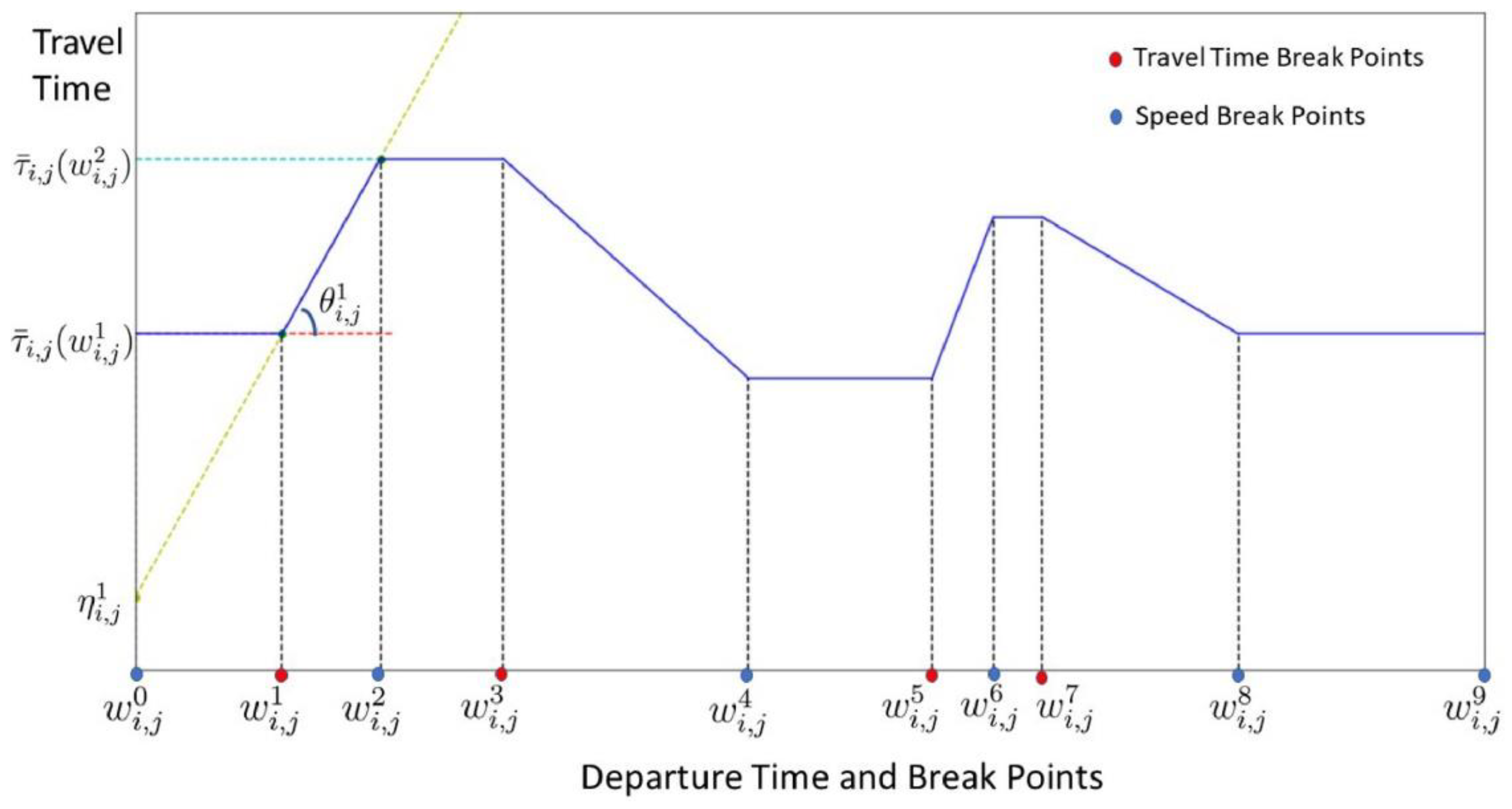
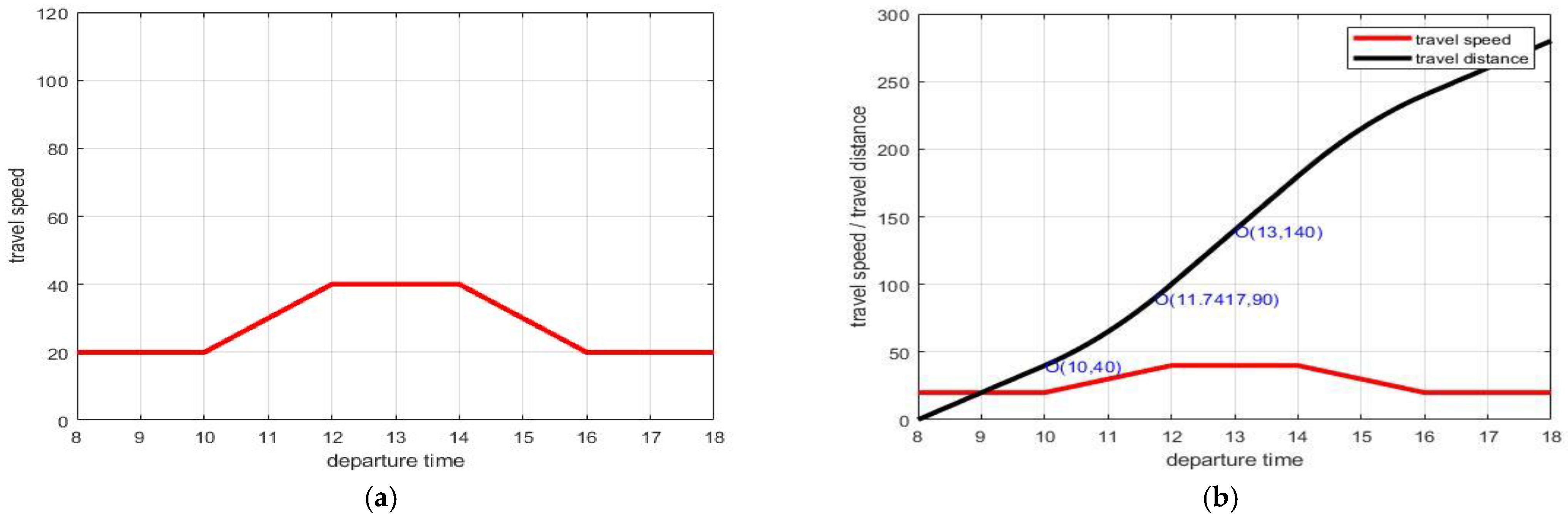
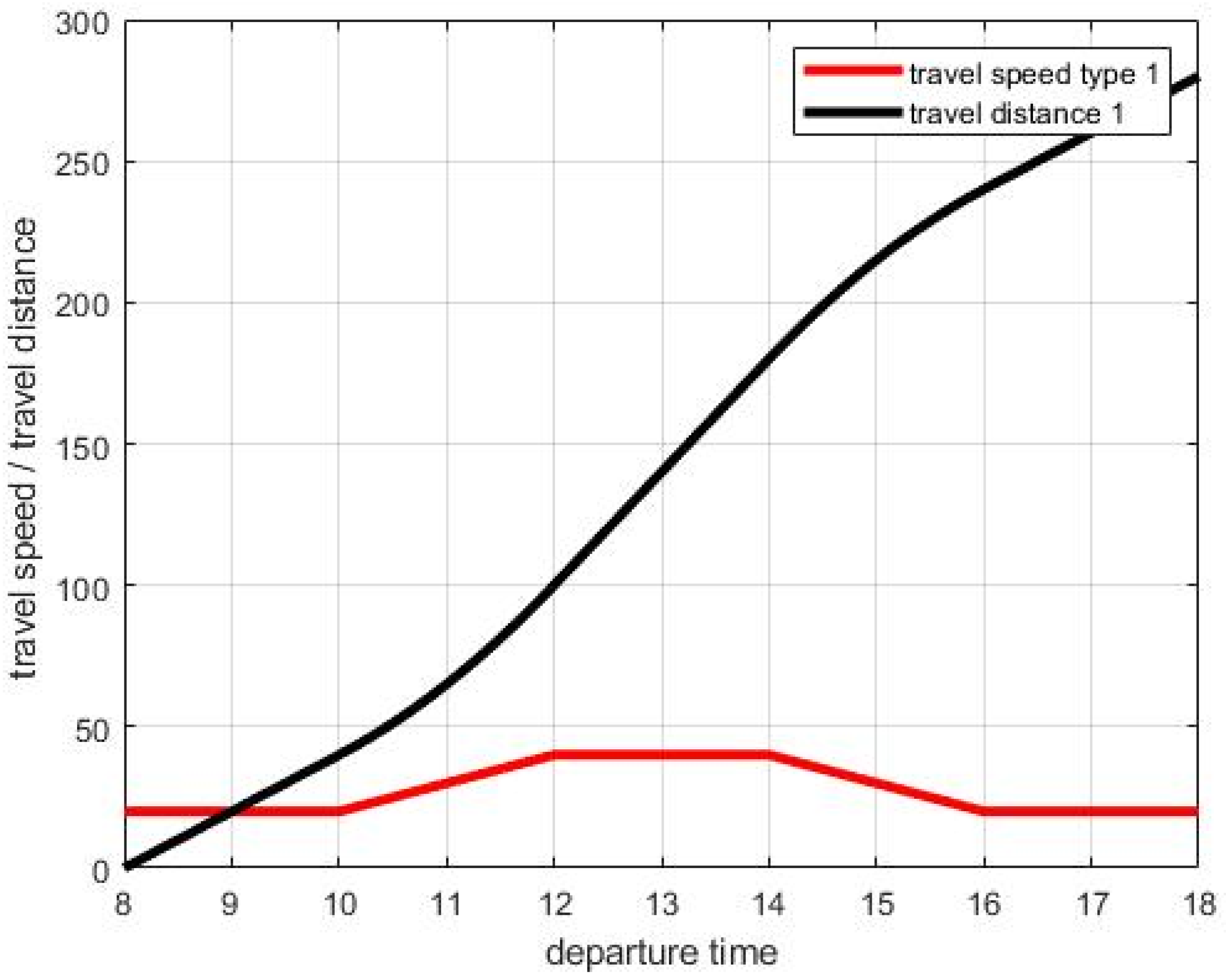
Even though many works in TDVRP have been carried out with time-varying speeds, the investigation carried out by the Texas A&M Transportation Institute Jha and Eisele [7] mentioned that the traveling speed increases or decreases smoothly, rather than treating it as a stepwise function. The drawbacks of this model are very obvious and, as shown in the Figure 2, will lead to breakpoints; although it can be said that the change in speed takes much less time than delivery at a constant speed. Hence, we present a time-varying speed model of a continuous function, as shown in the Figure 3a.

Proposition 1.

If the speed profile for an arc$\left(v_i, v_j\right)$is a stepwise linear continuous function, as show in Figure 3a, then the time-dependent travel distance function can be obtained by integrating the speed function, and the derived travel distance function is a continuous function, as depicted in Figure 3b.

Proposition 2.

Since travel distance corresponds to travel time one-to-one, then the time-dependent travel time function is the inverse function of travel distance. Using this one-to-one correspondence relationship, when the departure time and travel distance are known, the travel time can be calculated.

3.2. Heterogeneous Fixed Fleet Vehicle Routing Problem

Heterogeneous fleets VRPs (HVRPs) are considered a limited or unlimited fleet of capacitated vehicles, with problems, which consist of determining the fleet composition and vehicle routes (Koç, Bektaş, Jabali, and Laporte [39]). Let $M_m$ be the set of vehicles with m types, each type vehicle max available number be $ve{h}_m$, and subscript m be the type of vehicle (which will be used in the following text). The maximum load capacity of m type vehicle is $ca{p}_m$, the time-varying speed function of m type vehicle is $\mathrm{fun}-{\mathrm{speed}}_m\left(t_{dep,ij}\right)$, where $t_{dep,i}$ is the departure time from node i to node j, the time-varying travel time function is $\mathrm{fun}-{\mathrm{time}}_m\left(t_{dep,ij},d_{ij}\right)$, and $d_{ij}$ is the distance linking node i and node j, as mentioned before. Every type of car has a fixed cost $f{c}_m$, which is referred to as the cost of buying or renting, and a variable cost $v{c}_m$, used to express the cost per kilometer per kilogram of the weight of goods.

Assumptions

• The depot has a demand equal to zero
• Each customer location is serviced from only one vehicle
• Each customer’s delivery must arrive within the time window
• The number of each type of vehicle in routing cannot exceed each type of vehicle; the maximum available number is $ve{h}_m$
• Each vehicle shall not exceed its maximum load capacity $ca{p}_m$
• The total delivery time of each vehicle shall not exceed 9 h

Notations used in problem statement are defined as follows.

Detail model sets, indices, and parameters are shown in

Table 2. Sets, indices, and parameters.

Sets and Indices
V	$\mathrm{nodes} \mathrm{set}, v_0$$\mathrm{is} \mathrm{the} \mathrm{depot}, \left\{v_1, v_2, \dots , v_N\right\}$ are customers
i,j	$\mathrm{subscript} \mathrm{of} \mathrm{the} \mathrm{customer} \mathrm{node}, i,j=1,2,\dots N$
A	$\mathrm{A}=\left\{\left(v_i, v_j\right): v_i, v_j\in V\right\}$ is the arcs set linking node i and node j
$M_m$	the set of vehicles with m types
m	$\mathrm{vehicle} \mathrm{types}, m=1,2,\dots MK$
Parameters
$D_i$	demand of i customer
$t{w}_i$	$t{w}_i=\left[b_i, e_i\right]$ time window of i customer
$s_i$	service time of i customer
T	$\mathrm{T}=\left\{T_1, T_2, \dots , T_b\right\}$ time period
$t_{arr,i}$	the arrive time of node i
$t_{dep,ij}$	the departure time from node i to node j
$t_{tra,ij}$	the travel time from node i to node j
$d_{ij}$	the distance linking node i and node j
$\mathrm{fun}-{\mathrm{speed}}_m\left(t_{dep,ij}\right)$	time-varying speed function of m type vehicle
$\mathrm{fun}-{\mathrm{time}}_m\left(t_{dep,i},d_{ij}\right)$	time-varying travel time function of m type vehicle
$ve{h}_m$	each type of vehicle, maximum available number
$ca{p}_m$	maximum load capacity of m type vehicle
$f{c}_m$	fixed cost of m type vehicle
$v{c}_m$	variable cost of m type vehicle
$D{m}_{ij,m}$	amount carried using type m vehicle from i to j
Decision variable
$X_{ij,m}$	one if a type m vehicle travels from node i to j; otherwise, zero

.

3.3. Fitness Function and Mathematical Model

The traditional logistics model is concerned with minimizing total cost in a network. This is where the concept of Vehicle Routing Problem (VRP) is best applied. We follow this concept and add the fixed cost $f{c}_m$ of each type of vehicle into the total cost to minimize the total number of vehicles. We also include the variable cost $v{c}_m$ of delivery of each type of vehicle to optimize the vehicle scheduling. Other constraints appear in the target calculation in the form of penalty functions to enforce the constraints of the limit. The objective of minimizing the total cost is as follows:

$$\mathrm{Minimize} {\displaystyle \sum }_{m=1}^M{\displaystyle \sum }_{i=0}^N{\displaystyle \sum }_{j=0}^N{X}_{ij,m}{fc}_m+{\displaystyle \sum }_{m=1}^M{\displaystyle \sum }_{i=0}^N{\displaystyle \sum }_{j=0}^N{d}_{ij}{Dm}_{ij,m}{vc}_m$$

(1)

Subject to Routing

$${\displaystyle \sum }_{i=1}^N{X}_{i0,m}=1 \forall m \in M_m$$

(2)

$${\displaystyle \sum }_{m=1}^M{\displaystyle \sum }_{i=1}^N{\displaystyle \sum }_{j=1}^N{X}_{ij,m}=1 \forall \left(i,j\right)\in \mathrm{A} \forall m \in M_m$$

(3)

$${\displaystyle \sum }_{m=1}^M{\displaystyle \sum }_{i=1}^N{X}_{ip,m}={\displaystyle \sum }_{m=1}^M{\displaystyle \sum }_{i=1}^N{X}_{pi,m} \forall p \in V$$

(4)

Demand and Capacities

$${\displaystyle \sum }_{i=1}^N{\displaystyle \sum }_{j=1}^N{X}_{ij,m}{D}_j=D{m}_{ij,m} \forall \left(i,j\right)\in \mathrm{A} \forall m \in M_m$$

(5)

$${\displaystyle \sum }_{i=1}^{N}D{m}_{0i,m}\le ca{p}_m \forall m \in M_m$$

(6)

$${\displaystyle \sum }_{m=1}^M{X}_{ij,m}\le ve{h}_m \forall m \in M_m$$

(7)

Time Windows

$$t_{arr,j}=t_{dep,ij}+t_{tra,ij} \forall i,j\in \mathrm{V} \forall \left(i,j\right)\in \mathrm{A}$$

(8)

$$t_{arr,j}\in \left[b_j, e_j\right]$$

(9)

$$t_{dep,ij}=t_{arr,i}+s_i \forall i,j\in \mathrm{V}$$

(10)

$$t_{arr,0}<9\forall m \in M_m$$

(11)

The objective function (1) is total cost including fixed cost and variable cost. Constraint (2) defines that each vehicle should back to the Depot that subscript stands for 0. Constraint (3) ensures that each node can only be visited once in a route. Constraint (4) states that if a vehicle arrives at a node, it must leave it, and by this way, the route continuity is ensured. Constraints (10) and (11) state the restrictions for the amount of demand and capacities. Constraint (7) defines the maximum number of available vehicles $ve{h}_m$. Constraints (8) and (9) are the time window restrictions. Constraint (11) ensures that each vehicle cannot delivery over 9 h.

4. Simplified Swarm Optimization

As a generalization of VRP, the TDVRP and HFFVRP are also NP-hard and require intentional investigation for problem modeling and algorithmic design.

4.1. Simplified Swarm Optimization

SSO is one of the simplest machine-learning methods (Wang et al. [54,55,56] Yeh, et al. [57]) in terms of its update mechanism. It was first proposed by Yeh [27], and has been tested to be a very useful and efficient algorithm for optimization problems, including network reliability (Yeh [58] Yeh, et al. [59]), deep learning training (Yeh [60] Yeh, Lin, Liang and Lai [57]), disassembly sequencing problems (Yeh [61] Yeh [62]), energy problems (Lin et al. [63]), and so on. Owing to its simplicity and efficiency, SSO is used here to find the best values in vehicle routing of the proposed HFVRP with Time-Varying Continuous Speed Function.

The basic idea of SSO is that each variable, such as the jth variable in the ith solution x_i,j, needs to be updated based on the following stepwise function (Yeh [55,62]):

$$x_{i,j}=\{\begin{array}{cc}\begin{array}{c}{\mathrm{g}}_j\\ p_{i,j}\end{array}& \begin{array}{c}\mathrm{if} {\rho }_{\left[0,1\right]} \in \left[0, C_{\mathrm{g}}\right)\hfill \\ \mathrm{if} {\rho }_{\left[0,1\right]} \in \left[C_{\mathrm{g}}, C_p\right)\hfill \end{array}\\ \begin{array}{c}{x}_{i,j}\\ x\end{array}& \begin{array}{c}\mathrm{if} {\rho }_{\left[0,1\right]} \in \left[C_p, C_w\right)\hfill \\ \mathrm{if} {\rho }_{\left[0,1\right]} \in \left[C_w, 1\right)\hfill \end{array}\end{array}$$

(12)

where the value ρ_[0,1] ∈ [0,1] is generated randomly, the parameters C_g, C_p − C_g, C_w − C_p, 1 − C_w are all in [0,1] and are the probabilities of the current variable that are copied and pasted from the best of all solutions, the best ith solution, the current solution, and a random generated feasible value, respectively.

There are different variants of the traditional SSO that are customized to different problems from the no free lunch theorem; for example, the four items in Equation (11) are also reduced to three items to increase the efficiency; parameters C_g, C_p, and C_w are all self-adapted; special values or equations are implemented to replace g_j, p_i,j, x_i,j, and x; or only a certain number of variables is selected to be updated, etc. However, the SSO update mechanism is always based on the stepwise function.

4.2. Example for Code and Decode

To explain how the model works, a small instance from Vincent, Redi, Jewpanya, Lathifah, Maghfiroh, and Masruroh [43] was used for testing with 1 depot, 5 customers, and 3 types of vehicles. Table 1 shows the part of parameters for each vehicle from Vincent, Redi, Jewpanya, Lathifah, Maghfiroh, and Masruroh [43], since our research focus on the total cost which included fixed cost and variable cost, instead of the pollution cost in Vincent, Redi, Jewpanya, Lathifah, Maghfiroh, and Masruroh [43] study, some of the parameter settings have been omitted which can be known in detail in the Vincent, Redi, Jewpanya, Lathifah, Maghfiroh, and Masruroh [43] paper.

Table 3. Vehicle specification.

Notation	Description	Typical Values of a Type of m Vehicle
		Vehicle Type 1	Vehicle Type 2	Vehicle Type 3
$ca{p}_m$	Maximum load capacity of m type vehicle	1000	2000	3650
$v{c}_m$	Variable cost of m type vehicle (£/m)	0.0001	0.00015	0.0002

Note: $v{c}_m$ in the Vincent, Redi, et al. study did not consider the load of delivery

and

Table 4. Parameters for the small problem size.

	D	${\mathit{V}}_1$	${\mathit{V}}_2$	${\mathit{V}}_3$	${\mathit{V}}_4$	${\mathit{V}}_5$	Demand	${\mathit{b}}_{\mathit{i}}$	${\mathit{e}}_{\mathit{i}}$	${\mathit{s}}_{\mathit{i}}$
D	0	41,150	25,680	23,000	32,450	22,500	0	0	22,400	0
$V_1$	40,660	0	51,980	40,000	23,000	32,000	900	752	21,289	200
$V_2$	25,010	51,780	0	30,000	32,000	23,000	727	270	24,050	2000
$V_3$	20,000	30,000	300,000	0	23,000	25,000	800	250	22,500	1500
$V_4$	32,500	23,000	32,000	23,000	0	30,000	580	700	28,000	200
$V_5$	22,500	32,000	23,000	25,000	30,000	0	600	300	27,000	300

present the corresponding values for the distance matrix (in meters), demand, time window, and service time.

The route result given by the Vincent, Redi, et al. study is shown as follow

Route is 0-5-4-3-0, total distance is 95,500, vehicle type is type 2; Route II is 0-1-0, total distance is 81,810, vehicle type is type 1; Route III is 0-2-0, total distance is 50,690, vehicle type is type 1. Total distance of Route I, Route II, and Route III is 228,000, and total variable cost is 27.575

If code, this route result using SSO, first, should give each vehicle type the maximum available number $ve{h}_m$. Assume that each type of vehicle can complete the distribution task separately; since the total demand of customers is 3607, which requires $ve{h}_1=4, ve{h}_2=2, ve{h}_3=1$. According to the HFFVRP problem mentioned above, now, we need to decide the routing problem of 7 cars for 3 types of vehicles. And the representation using SSO is shown in

Table 5. Representation using SSO.

${\mathit{V}}_1$	${\mathit{V}}_2$	${\mathit{V}}_3$	${\mathit{V}}_4$	${\mathit{V}}_5$
1.2	2.1	5.3	5.2	5.1

.

The integer part of each number stands for the vehicle that will service, the same integer parts represent the same vehicle for serving the customers, and the order depends on value. For example, $V_3, V_4, V_5$ have the same integer parts, which means they are all delivered by vehicle 5 belong to type 2. The route is dependent on the value, since $5.1<5.2<5.3$, so the route of vehicle 5 is 0-5-4-3-0.

After an iterative update of SSO, the final solution is shown in the

Table 6. Cumulative result of small problem size; assume the velocity is 25 m/s.

From to	Distance	Travel time	Arrive T	TW	Service Time	Departure T
0–2	25,680	10,272	10,272	$\left[270, \mathrm{24,050}\right]$	2000	12,272
2–5	23,000	920	13,192	$\left[300, \mathrm{27,000}\right]$	300	13,492
5–1	32,000	1280	14,772	$\left[752, \mathrm{21,289}\right]$	200	14,972
1–4	23,000	920	15,892	$\left[700, \mathrm{28,000}\right]$	200	16,092
4–3	23,000	920	17,012	$\left[752, \mathrm{21,289}\right]$	1500	18,512
3–0	20,000	800	19,312	$\left[0, \mathrm{22,400}\right]$	0	/

.

The route is 0-2-5-1-4-3-0, service is by vehicle type 3, and the total distance is 146,680, which is much smaller than Vincent and Redi’s result. More importantly, the variable cost of Vincent and Redi’s model does not reflect the distribution cost caused by the load of the delivered goods, which is inconsistent with the actual distribution process

In practice, logistics companies will buy or rent vehicles with large volume ratings because the average variable cost per kilogram and per meter is lower due to the scale effect. For example, the average demand is 721.4, the average distance is 24,446.7 (take the best solution as an example), the variable cost will be a thousand, so we present a new parameters setting, as shown in

Table 7. New parameters setting.

Notation	Description	Typical Values of a Type of m Vehicle
		Vehicle Type 1	Vehicle Type 2	Vehicle Type 3
$ca{p}_m$	Maximum load capacity of m type vehicle	1000	2000	3650
$v{c}_m$	$\mathrm{Variable} \cos \mathrm{t} \mathrm{of} m \mathrm{type} \mathrm{vehicle} (\pounds /\mathrm{kg}·\mathrm{m}$)	0.00002	0.000015	0.00001
$f{c}_m$	Fixed cost of m type vehicle	50	100	180

, which will be used in the subsequent test indices, and new optimum route results as

Table 8. After new parameters setting-new optimum route.

From to	Distance	Total Dis	Variable Cost	Demand	Total VC
0–5	22,500	-	0.00002	600	270
5–0	22,500	-		1	0.45
0–2	25,680	-	0.000015	727	280.0404
2–0	25,010	-		1	0.3752
0–4	32,450	-	0.000015	580	282.315
4–0	32,500	-		1	0.4875
0–3	23,000	-	0.00001	800	184
3–1	30,000	53,000		900	477
1–0	40,660	-		1	0.4066
$\mathrm{Total} \cos \mathrm{t}=\mathrm{total} \mathrm{VC}+\mathrm{fix} \cos \mathrm{t} \mathrm{for} \mathrm{vehicle}$					1924.6995

.

New optimum route is shown as follow

Route I 0-5-0, delivery by vehicle type 1; Route II 0-2-0, delivery by vehicle type 2; Route III 0-4-0, delivery by vehicle type; Route IV 0-3-1-0, delivery by vehicle type 3.

4.3. SSO Algorithm Pseudo Code

In order to increase the speed of searching for the best solution, the part of inheriting the solution from the previous generation is cancelled, and the update mechanism is changed to

$$x_{i,j}=\{\begin{array}{cc}{\mathrm{g}}_j& \mathrm{if} {\rho }_{\left[0,1\right]} \in \left[0, C_{\mathrm{g}}\right)\hfill \\ p_{i,j}& \mathrm{if} {\rho }_{\left[0,1\right]} \in \left[C_{\mathrm{g}}, C_p\right)\hfill \\ x& \mathrm{otherwise}\end{array}$$

(13)

STEP 0. Initialize parameters; let $t=1$, randomly initial solution $S^1$.

Each variable for $S^t$ is $s_{nm}^t\in \left[1, mk\right]$, there are in total $mk$ vehicles, subscript n stands for n customer nodes, subscript m stands for m particle size, $d_i$ stands for customer i needs, $\left[b_i, e_i\right]$ stands for customer i time window.

STEP 1. Let $m=1$, first row of solution matrix.

STEP 1.1 Let $v=\mathrm{vehicle} \mathrm{order}=1$

STEP 1.2 Find $ve{h}_v=S_{nm}^t\in [v,v+1)$

STEP 1.3.1 Rank $ve{h}_v$ get $X_{ij}^1$, then read the distance $d_{ij}$ link node i and node j, add the $ve{h}_v$ vehicle fix cost;

STEP 1.3.2 calculate arrive time $t_{arr,i}$ for each node, and departure time $t_{dep,ij}=t_{arr,i}+s_i$ check whether the arrival time is in the time window.

STEP 1.3.3 calculate variable cost for each node,

STEP 1.3.4 check total weight not over $ca{p}_m$

STEP 1.4 Calculate $objec{t}_v$ for vehicle $ve{h}_v$

$objec{t}_v=\mathrm{fix} \cos \mathrm{t}+\mathrm{variable} \cos \mathrm{t}$

STEP 1.5

if $ve{h}_v<mk$

$ve{h}_v=ve{h}_v+1$, go back to STEP 1.2

Otherwise

Calculate $objec{t}_m^t={\displaystyle \sum }objec{t}_v$

If $Pbes{t}_m^t>objec{t}_m^t$

$Pbes{t}_m^t=objec{t}_m^t, Pbest{S}_m^t=S_m^t$ Otherwise

$Pbes{t}_m^t=Pbes{t}_m^t, Pbest{S}_m^t=Pbest{S}_m^t$ STEP 2.

if $m<\mathrm{popsize}$

$m=m+1$, go back to STEP 1.1

Otherwise

If $Gbes{t}^t>min\left(Pbes{t}_m^t\right)$

$Gbes{t}^t=min\left(Pbes{t}_m^t\right), Gbest{S}^t=min\left(Pbest{S}_m^t\right)$ Otherwise

$Gbes{t}^t=Gbes{t}^t, Gbest{S}^t=Gbest{S}^t$ STEP 3.

if $t<\mathrm{iteration}$ and CPU time is not met, randomly $\rho \in \left[node, popsize\right] \mathrm{and} x$

switch $\left({\rho }_{nm}\right)$

Case1 ${\rho }_{nm}\in [0,C_w=c_w)$

$s_{nm}^{t+1}=Gbest{S}^t$ Case2 ${\rho }_{nm}\in [C_w,C_p=C_w+c_p)$

$s_{nm}^{t+1}=Pbes{t}_m^t$ Case3 ${\rho }_{nm}\in [C_p,1]$

$s_{nm}^{t+1}=xt=t+1$

go back to STEP1

Otherwise

Halt

5. Computational Experiments

In this section, the experimental results are reported. First, the details for the results of the case study are presented. Next, the current solution obtained by the GA and PSO is used to compare with the results obtained by both the mathematical model and the algorithm. The benchmark instance is based on the Pollution Routing Problem dataset. The datasets are taken from http://www.apollo.management.soton.ac.uk/prplib.htm, accessed on 1 June 2021 (operating environment: Intel(R) Core(TM) i-74770K [email protected] GHz 3.50 GHz, memory 16.0 GB).

Vehicle setting as mentioned before, $v{c}_m$; unit change to ($\pounds /\mathrm{kg}·\mathrm{km}$) as shown in Table 7.

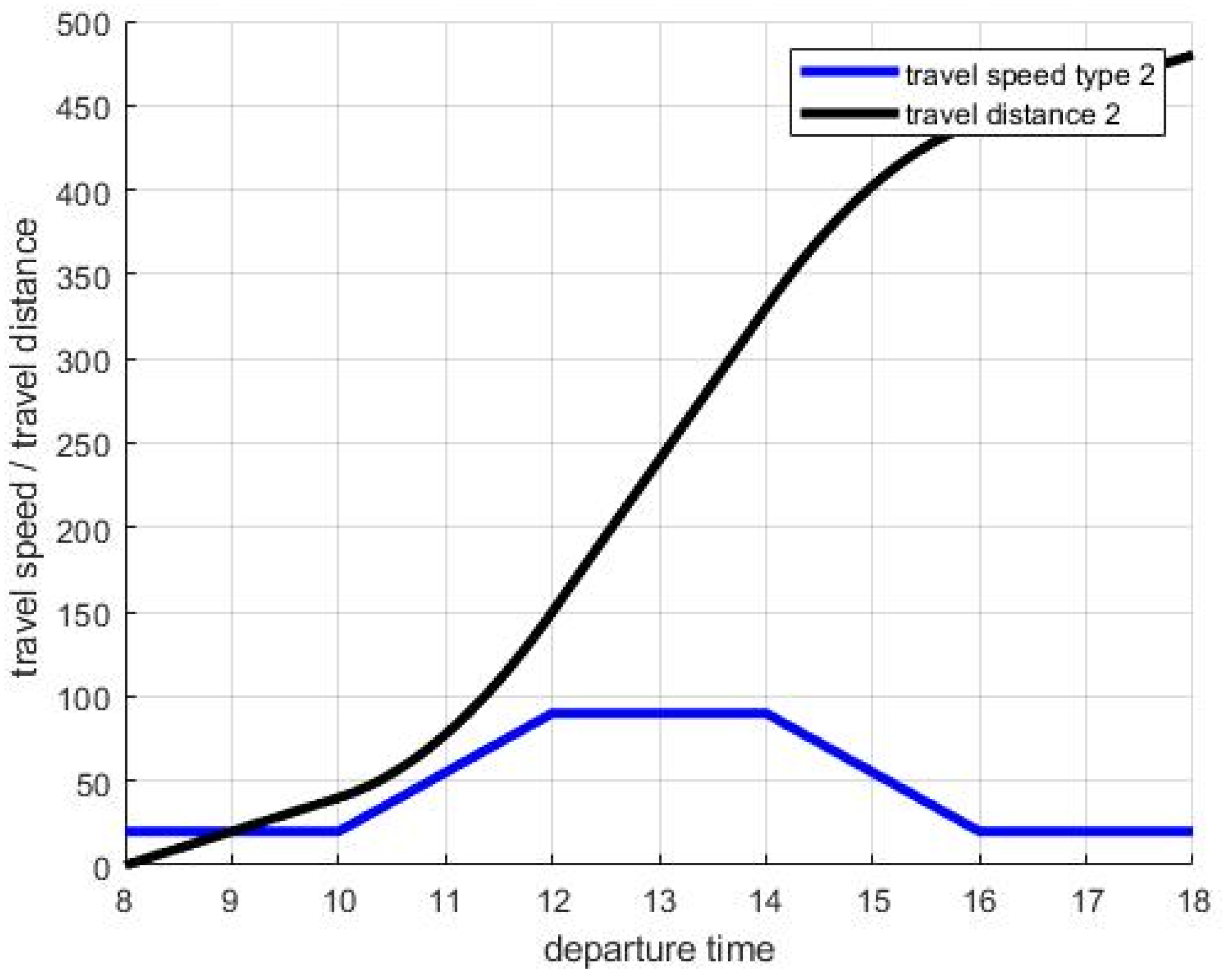
Vehicle type 1 belongs to “slow vehicle, travel speed type 1”; vehicle type 2, 3 belong to “quick vehicle, travel speed type 2”; the time-varying continuous travel speed function and time-varying travel time function are as in Figure 4, Figure 5 and Figure 6.

Take UK10_01, for example, to illustrate the calculation; the units are adjusted to kilometers and hours. After the adjustment, the service time can be ignored and is not considered in this study. The parameters after adjusted as show in the

Table 9. Parameters for the UK10_01.

	D	${\mathit{V}}_1$	${\mathit{V}}_2$	${\mathit{V}}_3$	${\mathit{V}}_4$	${\mathit{V}}_5$	${\mathit{V}}_6$	${\mathit{V}}_7$	${\mathit{V}}_8$	${\mathit{V}}_9$	${\mathit{V}}_{10}$	Dem	${\mathit{b}}_{\mathit{i}}$	${\mathit{e}}_{\mathit{i}}$
D	0	41	26	54	95	16	89	74	26	88	66	0	0	9
$V_1$	41	0	52	33	100	42	76	64	24	72	26	721	0.60	6.15
$V_2$	25	52	0	62	74	13	69	53	43	73	77	814	0.18	5.85
$V_3$	54	33	62	0	77	52	43	32	49	40	30	620	0.29	5.67
$V_4$	95	100	74	77	0	81	56	46	112	62	106	311	1.42	6.73
$V_5$	16	43	13	52	81	0	78	61	34	82	68	167	0.65	6.03
$V_6$	89	76	69	43	55	78	0	17	92	7	69	513	1.02	6.70
$V_7$	73	63	52	32	46	61	17	0	76	21	61	568	1.22	6.96
$V_8$	26	24	44	50	112	34	91	76	0	89	49	763	0.97	6.76
$V_9$	88	72	73	39	61	82	7	21	88	0	64	558	1.04	6.68
$V_{10}$	65	26	77	29	106	67	69	61	49	64	0	636	1.47	7.28

SSO is compared with GA and PSO, which have been widely used. The updating methods of GA and PSO can be referred to the papers of other authors: [21,22,24].

. The result comparison is shown is

Table 10. Result comparison.

	GA		PSO		SSO
	Average	Runtime	Average	Runtime	Average	Runtime
1	4744.389	28.758	5085.359	20.51	4734.099	18.478
2	4822.404	29.674	4959.387	20.772	4572.63	19.234
3	5155.445	29.27	5335.604	20.818	4856.664	18.736
4	4618.963	30.378	4959.715	20.876	4758.297	18.936
5	3786.287	29.118	4073.978	19.468	3866.133	19.302
6	4466.445	29.3425	4498.934	19.816	4345.842	19.004
7	3779.422	29.43	4002.631	19.738	3737.188	18.468
8	5735.288	29.826	5681.62	19.658	5673.156	18.868
9	4277.396	30.118	4349.053	19.214	3955.826	19.06
10	5411.929	28.9	5540.31	19.706	5383.005	19.288
average	4679.797	29.48145	4845.599	20.0576	4589.337	18.9374

From the result, bold is a better solution, shows that the SSO outperforms the original GA and PSO with respect to the average cost (run 5 times independently to take the average value) and runtime. In terms of runtime, SSO and PSO are close, slightly better than PSO. The objective value of the GA is also good, but it takes longer to run, due to the update mechanism of the GA.

.

Parameter setting of GA algorithm, the crossover rate and mutation rate are 0.6 and 0.4

Parameter setting of PSO algorithm, $\mathrm{w}=0.5, C_1=C_2=2$

Parameter setting of SSO algorithm, $C_g=0.5, C_p=C_w=0.75$,

More detailed information can be found in Appendix A.

6. Conclusions

In urban areas, traffic conditions show a discrepancy throughout the day and the travel time between two locations depends on the time of the day. Even though there are many discussions about the time-dependent model, few adopted the time-varying speed model which can better reflect different road time conditions and naturally satisfy the FIFO property. Thus, we present a novel model using the Time-Varying Continuous Speed Function to explain the time-varying traffic condition effect on delivery.

Moreover, in real conditions, a logistics company can choose a different vehicle to deliver the goods to minimize the total cost including fixed cost and variable cost. In our research, we proposed three types of vehicles with different capacities and costs. By comparing with [43], it is proved that our model can better reflect the actual distribution process and optimize vehicle selection and vehicle routing in the process of minimizing the total cost.

Owing to the complexity of the problem, we use SSO to address the proposed problem and use a Pollution Routing Problem dataset to validate it and compare the result with GA and PSO, which have been widely used in solving VRP problems. The results obtained from the analysis show that the SSO outperforms the original GA and PSO with respect to the total cost and runtime. We acknowledge some limitations in the current study, but these limitations also provide opportunities for further research: for example, applying the SSO to solve larger-scale problems. For the problem of the wide interval time window, path planning is not obviously constrained by the time window, and service time has little impact on distribution planning. Therefore, the problem of a narrow time window can be considered in the future.

References

- Cattaruzza, D.; Absi, N.; Feillet, D.; González-Feliu, J. Vehicle routing problems for city logistics. EURO J. Transp. Logist. 2017, 6, 51–79. [Google Scholar] [CrossRef]
- Dantzig, G.; Ramser, J. The Truck Dispatching Problem. Manag. Sci. 1959, 80–91. [Google Scholar] [CrossRef]
- Clarke, G.; Wright, J.W. Scheduling of vehicles from a central depot to a number of delivery points. Oper. Res. 1964, 12, 568–581. [Google Scholar] [CrossRef]
- Malandraki, C.; Daskin, M.S. Time dependent vehicle routing problems: Formulations, properties and heuristic algorithms. Transp. Sci. 1992, 26, 185–200. [Google Scholar] [CrossRef]
- Ichoua, S.; Gendreau, M.; Potvin, J.-Y. Vehicle dispatching with time-dependent travel times. Eur. J. Oper. Res. 2003, 144, 379–396. [Google Scholar] [CrossRef] [Green Version]
- Margiotta, R.; Eisele, B.; Short, J. Freight Performance Measure Approaches for Bottlenecks, Arterials, and Linking Volumes to Congestion Report. 2015. Available online: https://rosap.ntl.bts.gov/view/dot/41268 (accessed on 1 June 2021).
- Jha, K.; Eisele, B. Freight Multimodal Performance Measures. 2015. Available online: https://static.tti.tamu.edu/tti.tamu.edu/documents/TTI-2015-19.pdf (accessed on 1 June 2021).
- Baldacci, R.; Battarra, M.; Vigo, D. Routing a heterogeneous fleet of vehicles. In The Vehicle Routing Problem: Latest Advances and New Challenges; Springer: Berlin/Heidelberg, Germany, 2008; pp. 3–27. [Google Scholar]
- Taillard, É.D. A heuristic column generation method for the heterogeneous fleet VRP. RAIRO Oper. Res. Rech. Opér. 1999, 33, 1–14. [Google Scholar] [CrossRef] [Green Version]
- Wang, Z.; Wen, P. Optimization of a low-carbon two-echelon heterogeneous-fleet vehicle routing for cold chain logistics under mixed time window. Sustainability 2020, 12, 1967. [Google Scholar] [CrossRef] [Green Version]
- Anh, P.T.; Cuong, C.T.; Phuc, P.N.K. The vehicle routing problem with time windows: A case study of fresh food distribution center. In Proceedings of the 2019 11th International Conference on Knowledge and Systems Engineering (KSE), Da Nang, Vietnam, 24–26 October 2019; pp. 1–5. [Google Scholar]
- Adriano, D.D.; Montez, C.; Novaes, A.G.; Wangham, M. DMRVR: Dynamic milk-run vehicle routing solution using fog-based vehicular ad hoc networks. Electronics 2020, 9, 2010. [Google Scholar] [CrossRef]
- Yuan, Z.; Yang, Z.; Lv, L.; Shi, Y. A Bi-Level Path Planning Algorithm for Multi-AGV Routing Problem. Electronics 2020, 9, 1351. [Google Scholar] [CrossRef]
- Wang, Y.; Assogba, K.; Fan, J.; Xu, M.; Liu, Y.; Wang, H. Multi-depot green vehicle routing problem with shared transportation resource: Integration of time-dependent speed and piecewise penalty cost. J. Clean. Prod. 2019, 232, 12–29. [Google Scholar] [CrossRef]
- Emde, S.; Schneider, M. Just-in-time vehicle routing for in-house part feeding to assembly lines. Transp. Sci. 2018, 52, 657–672. [Google Scholar] [CrossRef]
- Liu, L.; Li, K.; Liu, Z. A capacitated vehicle routing problem with order available time in e-commerce industry. Eng. Optim. 2017, 49, 449–465. [Google Scholar] [CrossRef]
- Nakazawa, T.; Tang, S.; Obana, S. CCN-based inter-vehicle communication for efficient collection of road and traffic information. Electronics 2020, 9, 112. [Google Scholar] [CrossRef] [Green Version]
- Sujaree, K.; Samattapapong, N. A Hybrid Chemical Based Metaheuristic Approach for a Vaccine Cold Chain Network. Oper. Supply Chain Manag. Int. J. 2021, 14, 351–359. [Google Scholar] [CrossRef]
- Lenstra, J.K.; Kan, A.R. Complexity of vehicle routing and scheduling problems. Networks 1981, 11, 221–227. [Google Scholar] [CrossRef] [Green Version]
- Cordeau, J.-F.; Gendreau, M.; Laporte, G.; Potvin, J.-Y.; Semet, F. A guide to vehicle routing heuristics. J. Oper. Res. Soc. 2002, 53, 512–522. [Google Scholar] [CrossRef]
- Xu, Z.; Elomri, A.; Pokharel, S.; Mutlu, F. A model for capacitated green vehicle routing problem with the time-varying vehicle speed and soft time windows. Comput. Ind. Eng. 2019, 137, 106011. [Google Scholar] [CrossRef]
- Cao, S.; Liao, W.; Huang, Y. Heterogeneous fleet recyclables collection routing optimization in a two-echelon collaborative reverse logistics network from circular economic and environmental perspective. Sci. Total Environ. 2021, 758, 144062. [Google Scholar] [CrossRef]
- Fan, H.; Zhang, Y.; Tian, P.; Lv, Y.; Fan, H. Time-dependent multi-depot green vehicle routing problem with time windows considering temporal-spatial distance. Comput. Oper. Res. 2021, 129, 105211. [Google Scholar] [CrossRef]
- Alinaghian, M.; Ghazanfari, M.; Norouzi, N.; Nouralizadeh, H. A novel model for the time dependent competitive vehicle routing problem: Modified random topology particle swarm optimization. Netw. Spat. Econ. 2017, 17, 1185–1211. [Google Scholar] [CrossRef]
- Iswari, T.; Asih, A.M.S. Comparing genetic algorithm and particle swarm optimization for solving capacitated vehicle routing problem. IOP Conf. Ser. Mater. Sci. Eng. 2018, 337, 012004. [Google Scholar] [CrossRef]
- Yeh, W.-C. A hybrid heuristic algorithm for the multistage supply chain network problem. Int. J. Adv. Manuf. Technol. 2005, 26, 675–685. [Google Scholar] [CrossRef]
- Yeh, W.-C. A two-stage discrete particle swarm optimization for the problem of multiple multi-level redundancy allocation in series systems. Expert Syst. Appl. 2009, 36, 9192–9200. [Google Scholar] [CrossRef]
- Yeh, W.-C.; Chuang, M.-C. Using multi-objective genetic algorithm for partner selection in green supply chain problems. Expert Syst. Appl. 2011, 38, 4244–4253. [Google Scholar] [CrossRef]
- Malandraki, C.; Dial, R.B. A restricted dynamic programming heuristic algorithm for the time dependent traveling salesman problem. Eur. J. Oper. Res. 1996, 90, 45–55. [Google Scholar] [CrossRef]
- Çimen, M.; Soysal, M. Time-dependent green vehicle routing problem with stochastic vehicle speeds: An approximate dynamic programming algorithm. Transp. Res. Part D Transp. Environ. 2017, 54, 82–98. [Google Scholar] [CrossRef]
- Soysal, M.; Çimen, M. A simulation based restricted dynamic programming approach for the green time dependent vehicle routing problem. Comput. Oper. Res. 2017, 88, 297–305. [Google Scholar] [CrossRef]
- Sun, P.; Veelenturf, L.P.; Dabia, S.; Van Woensel, T. The time-dependent capacitated profitable tour problem with time windows and precedence constraints. Eur. J. Oper. Res. 2018, 264, 1058–1073. [Google Scholar] [CrossRef]
- Liu, C.; Kou, G.; Zhou, X.; Peng, Y.; Sheng, H.; Alsaadi, F.E. Time-dependent vehicle routing problem with time windows of city logistics with a congestion avoidance approach. Knowl. Based Syst. 2020, 188, 104813. [Google Scholar] [CrossRef]
- Pan, B.; Zhang, Z.; Lim, A. A hybrid algorithm for time-dependent vehicle routing problem with time windows. Comput. Oper. Res. 2021, 128, 105193. [Google Scholar] [CrossRef]
- Pan, B.; Zhang, Z.; Lim, A. Multi-trip time-dependent vehicle routing problem with time windows. Eur. J. Oper. Res. 2021, 291, 218–231. [Google Scholar] [CrossRef]
- Gmira, M.; Gendreau, M.; Lodi, A.; Potvin, J.-Y. Tabu search for the time-dependent vehicle routing problem with time windows on a road network. Eur. J. Oper. Res. 2021, 288, 129–140. [Google Scholar] [CrossRef]
- Xiao, Y.; Konak, A. The heterogeneous green vehicle routing and scheduling problem with time-varying traffic congestion. Transp. Res. Part E Logist. Transp. Rev. 2016, 88, 146–166. [Google Scholar] [CrossRef]
- Huang, C.-L.; Jiang, Y.-Z.; Tan, S.-Y.; Yeh, W.-C.; Chung, V.Y.Y.; Lai, C.-M. Simplified swarm optimization for the time dependent competitive vehicle routing problem with heterogeneous fleet. In Proceedings of the 2018 IEEE Congress on Evolutionary Computation (CEC), Rio de Janeiro, Brazil, 8–13 July 2018; pp. 1–8. [Google Scholar]
- Koç, Ç.; Bektaş, T.; Jabali, O.; Laporte, G. Thirty years of heterogeneous vehicle routing. Eur. J. Oper. Res. 2016, 249, 1–21. [Google Scholar] [CrossRef] [Green Version]
- Golden, B.; Assad, A.; Levy, L.; Gheysens, F. The fleet size and mix vehicle routing problem. Comput. Oper. Res. 1984, 11, 49–66. [Google Scholar] [CrossRef]
- Micheli, G.J.; Mantella, F. Modelling an environmentally-extended inventory routing problem with demand uncertainty and a heterogeneous fleet under carbon control policies. Int. J. Prod. Econ. 2018, 204, 316–327. [Google Scholar] [CrossRef]
- Afshar-Nadjafi, B.; Afshar-Nadjafi, A. A constructive heuristic for time-dependent multi-depot vehicle routing problem with time-windows and heterogeneous fleet. J. King Saud Univ. Eng. Sci. 2017, 29, 29–34. [Google Scholar] [CrossRef] [Green Version]
- Vincent, F.Y.; Redi, A.P.; Jewpanya, P.; Lathifah, A.; Maghfiroh, M.F.; Masruroh, N.A. A simulated annealing heuristic for the heterogeneous fleet pollution routing problem. In Environmental Sustainability in Asian Logistics and Supply Chains; Springer: Berlin/Heidelberg, Germany, 2019; pp. 171–204. [Google Scholar]
- Wang, Z.; Qi, M.; Cheng, C.; Zhang, C. A hybrid algorithm for large-scale service network design considering a heterogeneous fleet. Eur. J. Oper. Res. 2019, 276, 483–494. [Google Scholar] [CrossRef]
- De, M.; Giri, B. Modelling a closed-loop supply chain with a heterogeneous fleet under carbon emission reduction policy. Transp. Res. Part E Logist. Transp. Rev. 2020, 133, 101813. [Google Scholar] [CrossRef]
- Soman, J.T.; Patil, R.J. A scatter search method for heterogeneous fleet vehicle routing problem with release dates under lateness dependent tardiness costs. Expert Syst. Appl. 2020, 150, 113302. [Google Scholar] [CrossRef]
- Ropke, S.; Cordeau, J.F. Branch and cut and price for the pickup and delivery problem with time windows. Transp. Sci. 2009, 43, 267–286. [Google Scholar] [CrossRef] [Green Version]
- Ben Ticha, H.; Absi, N.; Feillet, D.; Quilliot, A. Vehicle routing problems with road-network information: State of the art. Networks 2018, 72, 393–406. [Google Scholar] [CrossRef]
- Crainic, T.G.; Frangioni, A.; Gendron, B. Bundle-based relaxation methods for multicommodity capacitated fixed charge network design. Discret. Appl. Math. 2001, 112, 73–99. [Google Scholar] [CrossRef]
- Shelbourne, B.C.; Battarra, M.; Potts, C.N. The vehicle routing problem with release and due dates. INFORMS J. Comput. 2017, 29, 705–723. [Google Scholar] [CrossRef]
- Xu, Z.; Ming, X.; Zheng, M.; Li, M.; He, L.; Song, W. Cross-trained workers scheduling for field service using improved NSGA-II. Int. J. Prod. Res. 2015, 53, 1255–1272. [Google Scholar] [CrossRef]
- Vidal, T.; Crainic, T.G.; Gendreau, M.; Lahrichi, N.; Rei, W. A hybrid genetic algorithm for multidepot and periodic vehicle routing problems. Oper. Res. 2012, 60, 611–624. [Google Scholar] [CrossRef]
- Zhong, S.-Q.; Du, G.; He, G.-G. Study on open vehicle routing problem with time windows limits and its genetic algorithm. Jisuanji Gongcheng Yu Yingyong Comput. Eng. Appl. 2006, 42, 201–204. [Google Scholar]
- Wang, M.; Yeh, W.-C.; Chu, T.-C.; Zhang, X.; Huang, C.-L.; Yang, J. Solving multi-objective fuzzy optimization in wireless smart sensor networks under uncertainty using a hybrid of IFR and SSO algorithm. Energies 2018, 11, 2385. [Google Scholar] [CrossRef] [Green Version]
- Yeh, W.-C.; Lai, C.-M.; Peng, Y.-F. Multi-objective optimal operation of renewable energy hybrid CCHP system using SSO. J. Phys. Conf. Ser. 2019, 1411, 012016. [Google Scholar] [CrossRef]
- Lai, C.-M.; Chiu, C.-C.; Liu, W.-C.; Yeh, W.-C. A novel nondominated sorting simplified swarm optimization for multi-stage capacitated facility location problems with multiple quantitative and qualitative objectives. Appl. Soft Comput. 2019, 84, 105684. [Google Scholar] [CrossRef]
- Yeh, W.-C.; Lin, Y.-P.; Liang, Y.-C.; Lai, C.-M. Convolution Neural Network Hyperparameter Optimization Using Simplified Swarm Optimization. arXiv 2021, arXiv:2103.03995. [Google Scholar]
- Yeh, W.-C. A novel boundary swarm optimization method for reliability redundancy allocation problems. Reliab. Eng. Syst. Saf. 2019, 192, 106060. [Google Scholar] [CrossRef]
- Yeh, W.-C.; Su, Y.-Z.; Gao, X.-Z.; Hu, C.-F.; Wang, J.; Huang, C.-L. Simplified swarm optimization for bi-objection active reliability redundancy allocation problems. Appl. Soft Comput. 2021, 106, 107321. [Google Scholar] [CrossRef]
- Yeh, W.-C. New parameter-free simplified swarm optimization for artificial neural network training and its application in the prediction of time series. IEEE Trans. Neural Netw. Learn. Syst. 2013, 24, 661–665. [Google Scholar] [PubMed]
- Yeh, W.-C. Optimization of the disassembly sequencing problem on the basis of self-adaptive simplified swarm optimization. IEEE Trans. Syst. Man Cybern. Part A Syst. Hum. 2011, 42, 250–261. [Google Scholar] [CrossRef]
- Yeh, W.-C. Simplified swarm optimization in disassembly sequencing problems with learning effects. Comput. Oper. Res. 2012, 39, 2168–2177. [Google Scholar] [CrossRef]
- Lin, P.; Cheng, S.; Yeh, W.; Chen, Z.; Wu, L. Parameters extraction of solar cell models using a modified simplified swarm optimization algorithm. Sol. Energy 2017, 144, 594–603. [Google Scholar] [CrossRef]
Figure 1.
(a) Travel time function on a link; (b) travel speed function at a node.
Figure 2.
Travel time function.
Figure 3.
(a) Time-varying continuous travel speed function; (b) travel distance function.
Figure 4.
Time-varying continuous travel speed function for 2 types of vehicles.
Figure 5.
Time-varying travel time function for “slow vehicle”.
Figure 6.
Time-varying travel time function for “quick vehicle’.