
Integrating Vehicle Positioning and Path Tracking Practices for an Autonomous Vehicle Prototype in Campus Environment


1
Department of Electrical Engineering, National Taiwan University of Science and Technology, Taipei 106335, Taiwan
2
Department of Mechanical Engineering, National Taiwan University, Taipei 10617, Taiwan
*
Author to whom correspondence should be addressed.
Electronics 2021, 10(21), 2703; https://0-doi-org.brum.beds.ac.uk/10.3390/electronics10212703
Submission received: 6 September 2021
/
Revised: 1 November 2021
/
Accepted: 3 November 2021
/
Published: 5 November 2021
(This article belongs to the Special Issue Unmanned Vehicles and Intelligent Robotic Alike Systems)
Abstract
:This paper presents the implementation of an autonomous electric vehicle (EV) project in the National Taiwan University of Science and Technology (NTUST) campus in Taiwan. The aim of this work was to integrate two important practices of realizing an autonomous vehicle in a campus environment, including vehicle positioning and path tracking. Such a project is helpful to the students to learn and practice key technologies of autonomous vehicles conveniently. Therefore, a laboratory-made EV was equipped with real-time kinematic GPS (RTK-GPS) to provide centimeter position accuracy. Furthermore, the model predictive control (MPC) was proposed to perform the path tracking capability. Nevertheless, the RTK-GPS exhibited some robust positioning concerns in practical application, such as a low update rate, signal obstruction, signal drift, and network instability. To solve this problem, a multisensory fusion approach using an unscented Kalman filter (UKF) was utilized to improve the vehicle positioning performance by further considering an inertial measurement unit (IMU) and wheel odometry. On the other hand, the model predictive control (MPC) is usually used to control autonomous EVs. However, the determination of MPC parameters is a challenging task. Hence, reinforcement learning (RL) was utilized to generalize the pre-trained datum value for the determination of MPC parameters in practice. To evaluate the performance of the RL-based MPC, software simulations using MATLAB and a laboratory-made, full-scale electric vehicle were arranged for experiments and validation. In a 199.27 m campus loop path, the estimated travel distance error was 0.82% in terms of UKF. The MPC parameters generated by RL also achieved a better tracking performance with 0.227 m RMSE in path tracking experiments, and they also achieved a better tracking performance when compared to that of human-tuned MPC parameters.
1. Introduction
Vehicle positioning and path tracking are essential to the development of autonomous vehicles. Vehicle positioning is responsible for providing stable, real-time, and accurate location information for navigations. The path tracking is developed to navigate the vehicle by following the desired trajectory to reduce the tracking errors. In general, the position accuracy with a conventional, stand-alone global positioning system (GPS) is approximately 0.5 m to 3.5 m on average. By applying real-time kinematic (RTK) technology, the GPS positioning accuracy can be improved to the centimeter level. However, the RTK-GPS performance is still restricted when jumping and drifting occur in an obstructed area, such as a blockage and multipath effects in an urban region with buildings and landscapes, under a bridge, or in a tunnel.
Due to the aforementioned RTK-GPS limitations, wheel odometry and inertial measurement units (IMUs) were complementarily combined with the global navigation satellite system (GNSS) to realize a stable and accurate multisensory, fusion-based vehicle positioning system. The aforementioned multisensory fusion problem is nonlinear; hence, an extended Kalman filter (EKF) or unscented Kalman filter (UKF) could be considered. However, the UKF outperforms the conventional EKF in terms of accuracy performance at a comparable level of system complexity [1]. Hence, this work used the UKF as the vehicle position estimation.
On the other hand, a commonly used model predictive control (MPC) method in a dynamic vehicle control system was further utilized in this work. The MPC controller calculates the system output according to the linear time-varying (LTV) model. Nevertheless, due to vehicle dynamics, hardware limitations, and environmental disturbances, system stability and trajectory tracking accuracy were a challenge. The MPC parameter settings are highly related to the controller performance. Practically, trial-and-error blind tuning of MPC parameters takes time and is inefficient. Therefore, applying reinforcement learning (RL) is a helpful way to produce proper MPC parameters to improve the trajectory tracking performance in terms of defining the rewards, states, and actions. Such an RL model works based on the tuning experience of the human MPC model parameters. The pre-trained MPC parameters are capable of providing the datum value rather than trial-and-error. As a consequence, the MPC parameters generated by the RL methods efficiently and effectively supported the MPC to perform an accurate path tracking performance. Such MPC performance measures were evaluated in terms of a simulation environment and a laboratory-made, full-scale electric vehicle.
The rest of the paper is organized as follows. Section 2 surveys the related works. The methods regarding the system architecture, vehicle model, implementation of the UKF-based position estimation, and the RL-based MPC algorithm are discussed in Section 3. In Section 4, the simulation of the proposed system and experiments on the evaluations of the position estimator and RL-based MPC trajectory tracking with a full-scale EV are elaborated. Finally, the conclusion of the proposed study and future works are presented in Section 5.
2. Related Works
This paper first surveys the related works within vehicle positioning. In general, a stand-alone GPS could suffer from a signal mismatch or failure. In addition, inaccurate GPS positioning cannot be directly applied to autonomous vehicle driving purposes unless extra efforts are made, such as image-based lane detection methods [2]. RTK-GPS provides a center centimeter level, and it has been widely used in low-speed (1 Hz) surveying and mapping systems. With the RTK (fixed mode), the position error may be less than 10 cm by following the radiotechnical commission for maritime (RTCM) service standards. Furthermore, the strength of the signal must be larger than 40 dB, and it is expected to receive 16 satellites normally to meet the lowest requirements [3].
Practically, the RTK-GPS is basically composed of a fixed base station and a rover to reduce the rover’s positioning error. Hence, communication between the base station and the rover must be established. An RF module is convenient; however, the disadvantage of utilizing RF modules is that the transmission distance might be limited by the rated power or environment interference. Hence, the stability of signal transmission using RF modules is a challenge [4].
When applying RTK-GPS as a solution to autonomous driving, low-evaluation satellites may suffer from larger atmospheric errors. Practically, implementation with a Kalman filter (KF) estimation could obtain integer ambiguities that allow individuals to be corrected by all ambiguity parameters in practical applications [5]. Moreover, the performance of RTK-GPS may be limited when driving in an interferential environment. The performance evaluation method could be performed in terms of statistically comparing the traveled path by using the mean absolute error and the root mean square (RMS) error, as addressed in [6].
Network instability and component failure are concerns of applying RTK-GPS in practical usages. Hence, Um et al. [7] proposed a redundancy solution, and their system could switch the master system to one of the available slave systems to deal with such network or component failures. In addition, the GPS accuracy may drop due to the multipath error that could occur during signal reflections among large amounts of objects. Therefore, the GSA message was used to provide position dilution of precision (PDOP) measurements according to the geometric constellation of GPS satellites [8,9].
Based on the NMEA (National Electrical Manufacturers Association) GST instructions, the standard deviations of latitude and longitude values are known. Such information could be applied for EKF-based visual odometry and GPS sensor fusion solutions. Once the measurement data are convincing enough, the visual odometry position can be corrected by GPS [10]. Furthermore, the transformation matrix of GPS can be determined to transform the local tangent plane (LTP) coordinates to world coordinates [11]. Within the considerations of the RTK carrier phase ambiguities and the pseudorange multipath errors, the state prediction could be more robust and precise [12]. Odometry methods are categorized into five main types, i.e., wheel, inertial, laser, radar, and visual. Most of the research applied multiple sensors to fuse or optimize the estimation of vehicle position [13].
In general, accumulative error is a critical factor of odometry. Hence, Mikov et al. [14] integrated inertial MEMS (Micro-Electromechanical Systems) and odometry solutions for land vehicle localizations. When the GNSS (Global Navigation Satellite System) signal is available, it can become the odometry correction factor to fix the position. The characteristics of GNSS and IMU are complementary, and they are fused in terms of KFs. Their results achieved a higher sampling rate and a high bandwidth by utilizing an online error state covariance estimation [15]. In addition to the EKF, the UKF is suitable for solving nonlinear problems. The advantage of using the UKF is that it does not need to calculate the Jacobian matrix and apply Taylor expansion. Hence, the UKF eventually results in a higher precision of estimation.
In addition to vehicle positioning, the related works within path tracking problems are also discussed. The single-track kinematics model is simple, and it is often applied to the MPC controller design. The optimal steering wheel angle and longitudinal force can be obtained by using the standard quadratic cost function based on the design constraints [16,17,18]. Under different speed ranges, the prediction model needs to be robust enough to describe the overall vehicle motion behaviors; otherwise, the prediction error will significantly increase [19].
Tang et al. [20] presented the lane changing control method in highway environments. Their study applied MPC as a controller for lane changing path planning. A multi-constraint model predictive control algorithm and optimization for lane changing were proposed. By determining the Q and R cost coefficients in the MPC model, the objective function can be minimized after the iterations. Assuming that the path tracking controller and driver behavior can be synthesized, the robustness and performance of driver-oriented maneuvers, such as cutting in and overtaking, can be further improved [21,22].
Optimization-based autonomous racing RC (Remote Control) cars were also carried out in [23]. That study combined the multitask problem as a nonlinear optimization problem (NLP) for contouring control. The proposed control system was created to build local approximations of NLPs in convex quadratic programs (QPs) at each time step. The algorithm solved the constrained infinite horizon optimal control problem at each time step and iteration. Moreover, an approximated safe set was added to satisfy the real-time computation and to prevent the occurrence of insoluble solutions [24]. The recursive least square algorithm and first-order Lagrange interpolation can be used to further estimate the cornering stiffness and road friction [25].
On the other hand, MPC is highly dependent on the prediction model. The properties of MPC and reinforcement learning (RL) are quite different but complementary, such as model requirements, robustness, stability, feasibility, etc. [26]. The RL applied the concept of the Markov decision process. Based on this assumption, the whole model can be simplified and the next state can be estimated [27].
The combination of RL and MPC was successfully applied to connected and automated vehicles at intersections [28]. The trained coordinate policy in a simulation setting and proximal policy optimization were applied. Their results demonstrated that the computing time and traffic efficiency outperformed other works. Another work [29] was proposed by Tange et al. Their study proposed model predictive control based on the deep RL approach. By evaluating the control performance and learning convergence, their discrete-valued input deep RL method achieved a better performance than direct P-based and PI-based RL methods.
Finally, parameter tuning could be applied by RL methods in various fields. A segmented and adaptive RL approach was proposed in [30] to provide successful noise reduction. By searching possible solution spaces, all the coefficient values can be well tuned in a short learning time. Such an RL-based parameter tuning concept is also applied in this paper to find the MPC parameters.
3. Methods
3.1. System Architecture
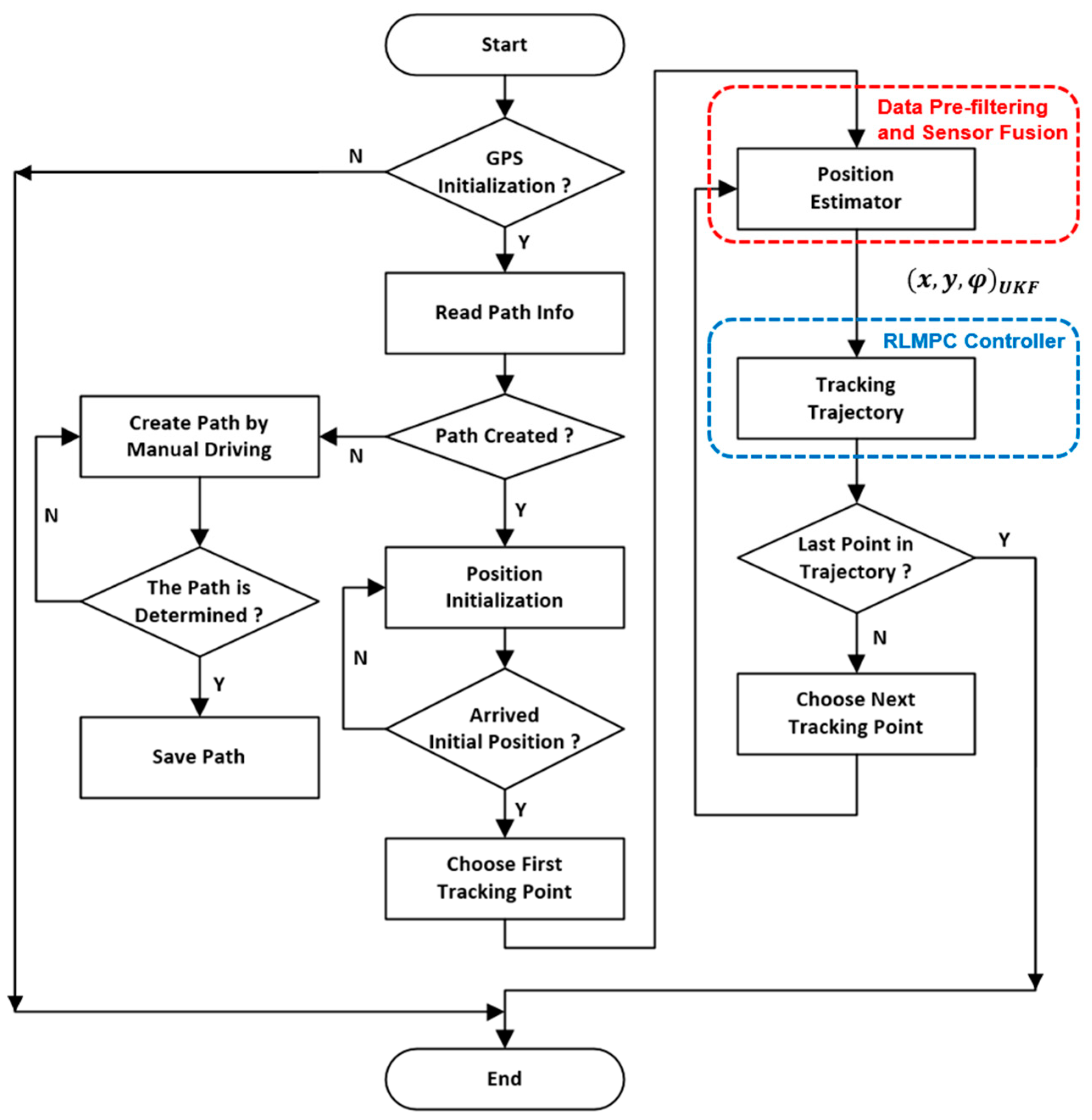
The overall system is primarily composed of a UKF-based position estimator and an RL-based MPC (RLMPC) controller design. The Robot Operating System (ROS) system was used in this work to develop all the programs. The first part addressed the UKF-based vehicle positioning system, and stable and accurate vehicle position information was further used for path tracking. The overall operation flowchart of this study is shown in Figure 1.
When the operator intends to start the autonomous driving function, the initialization of the GPS device needs to be ensured. Once the RTK correction signal is received and set, the electric vehicle (EV) is ready for operation. It is noted that the 4G communication modules are convenient to provide a stable signal transmission channel between the base station and the rover.
Autonomous driving also must ensure that the desired navigation path is created. If the path file is not found, a vehicle mission path file can be created either by recording the manual drive path by receiving the UKF vehicle positions or by planning. After the mission path file is loaded, the EV can start the navigation mission at any arbitrary location near the path start location of the trip. The mission task is divided into two parts: The first part is to autonomously drive from the vehicle initial position to the desired path start location; the second part is the path mission part, and the RLMPC controller is capable of tracking the desired trajectory from the path start location to the path destination location by maintaining minimum tracking error. The details of UKF position estimation and RLMPC path tracking will be explained in detail in Section 3.3 and Section 3.4.
3.2. Vehicle Modeling
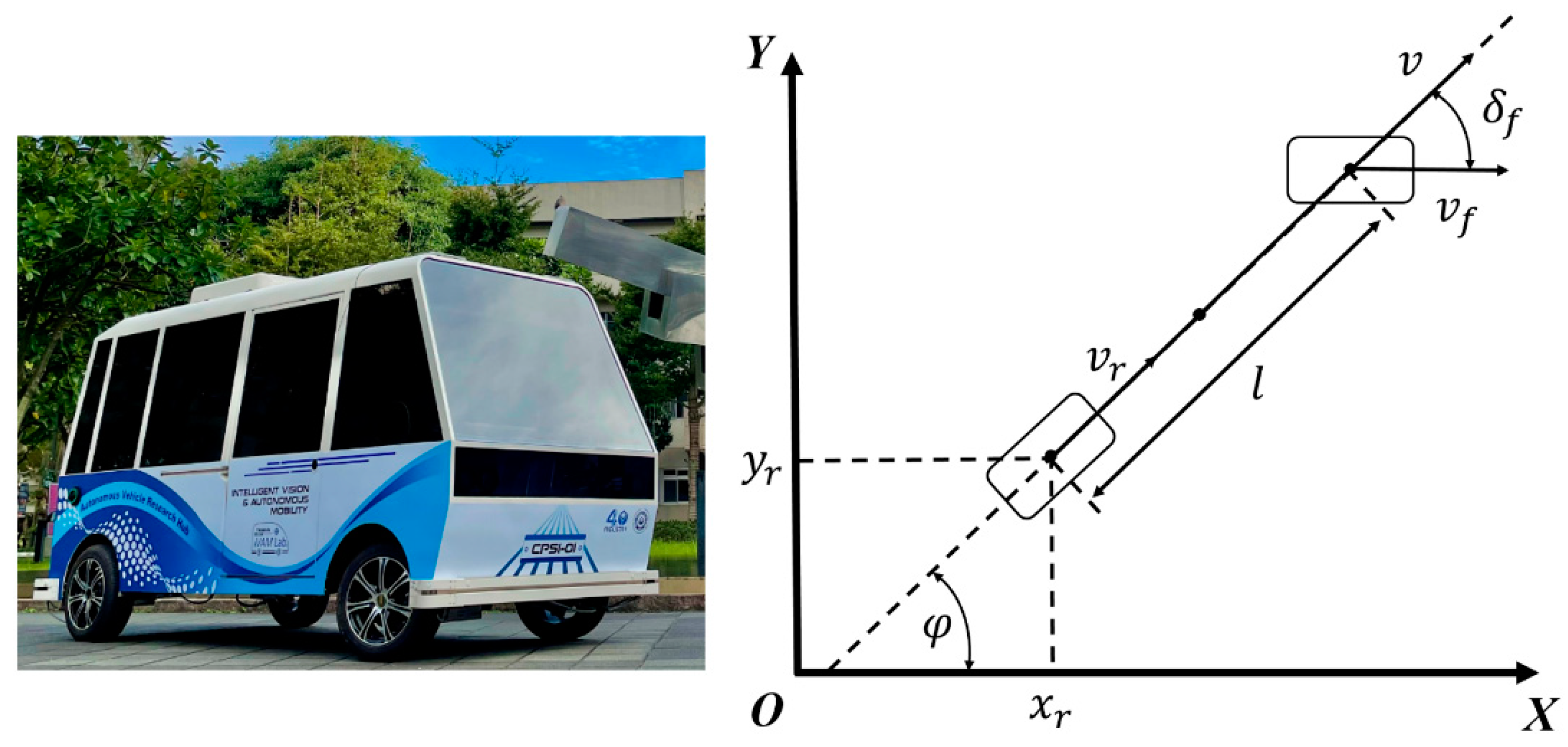
To evaluate the performance of vehicle positioning and path tracking, a full-scale, laboratory-made electric vehicle (EV) was used for experiments on the campus of National Taiwan University of Science and Technology (NTUST). A kinematic bicycle model was applied since the steering geometry and the control maneuvers can only fit at low speeds and low lateral acceleration in the campus experimental setting. The EV for experiments is shown on the left-hand side of Figure 2. The dimensions of the EV were 3.57 m (L) × 1.55 m (W) × 1.87 m (H), and the vehicle was 1300 kg in weight. The maximum speed was 30 km/h to meet the campus driving setting. The RTK-GPS receiver was installed on the top center of the vehicle. The rotary encoders were mounted inside two rear motors, and the IMU was fixed in front of the EV. It is noted that two 2-D outdoor usage lidars placed inside the right front and left rear of the front and rear bumpers were used to form a 360° detection of obstacles for collision avoidance. Because reactive obstacle avoidance was not the purpose of this paper, the vehicle temporarily stopped autonomous navigation when any obstacles were detected from two LiDars within a 2 m range for safety.
Based on the EV model, the inertial reference frames OXY, and were the coordinates at the front axle and rear axle, respectively, as shown on the right-hand side of Figure 2, where is the vehicle heading angle, , and it is the magnitude of the velocity vector of the center mass, and are the center velocities of the front axle and rear axle, respectively, and are the distances to the front axle and rear axle from the center of mass, respectively, is the distance from the front axle to the rear axle, and is the steering angle. It was assumed that there was no slip between the road and the tire for low-speed campus driving. The velocity model can be obtained in Equations (1) and (2).
From Equations (1) and (2), the vehicle kinematic model can be derived in Equation (3)
The kinematic bicycle model can be denoted in a generalized form . The state is and the control vector is .
3.3. UKF-Based Position Estimation
In this subsection, the position estimator consisted of two steps: (1) data prefiltering and (2) multisensory fusion. To accomplish the prefiltering of the poor data point, the covariance matrices were defined as the inverse matrix of the covariance matrix of RTK (Crtk) and the covariance matrix of odometry (Codm). The vectors collected from stand-alone RTK-GPS and odometry were and , respectively. The sampling rates of the RTK and odometry were 1 Hz and 10 Hz, respectively. Due to the different sampling rates of the sensors, orientation jumping occurred severely. Hence, in this paper, the Mahalanobis distances and are defined independently as Equations (4) and (5). In addition, the covariance matrices are defined in Equations (6) and (7).
Within the RTK data, the covariance matrix and the standard deviation were obtained by the fixed-point experiments, and they were compared with the GGA as well as the VTG message from the NMEA standard. Practically, it was impossible to obtain an accurate position when the vehicle was traveling. This is the reason why the statistical data were measured by fixed points. Meanwhile, the covariance matrix and standard deviation were based on the experiments that drove through a fixed distance, and they were calculated from the recorded data.
Moreover, and are the measurement errors, which need to be lower than the threshold values of and . The validation criterion depends on the threshold values, and a lower results in stricter judgment. During the iteration, once the measured error is lower than , the sample point will be inputted to the UKF framework. Otherwise, the sample point will be ignored. In this paper, the threshold values for the proposed EV are and . Both settings were determined by empirical knowledge in this model. By applying the above rules, the pre-filtered data points can be divided into four types, which are described as follows.
- Case 1: If and , the correction set of will take into account both position and orientation data from odometry, where and the covariance matrix of measurement noise are defined as in Equations (8) and (9):
- Case 2: If and , the correction set of will only take the position data from odometry, where and the covariance matrix of measurement noise are defined as in Equations (10) and (11):It is noted that is the estimated orientation of the UKF from the last iteration.
- Case 3: If and , the correction set of will only take the orientation data from odometry, where and the covariance matrix of measurement noise are defined as in Equations (12) and (13):It is noted that and are the components of the estimated position of the UKF from the last iteration.
- Case 4: If and , the vehicle will not take the odometry measurement data as the correction input of the UKF.
After the above processes, the pre-filtered data point can be obtained, and it will be used as the observation of UKF frameworks.
It is noted that the UKF worked at 10 Hz in this work. Based on the unscented transformation (UT), the use of sigma points to describe the nonlinear system would not sacrifice the high-order terms that make the system more precise. Compared with the EKF, the UKF can achieve higher efficiency and marvelous performance without calculating the Jacobian matrix and applying the Tylor expansion. The UKF iteration includes prediction and update processes. The UKF is briefly introduced [1]. Assume that there is a discrete-time, nonlinear system, as in Equation (14).
where and represent the dynamic model of the nonlinear systems, and they are assumed to be known, is the unobserved state of the system, is the system input, is the only observed state, is the process noise, and is the measurement noise of the system observation. When the variable with dimension L goes through a nonlinear system , has the mean and the covariance . Then, a matrix called a sigma matrix with size 2L + 1 is formed. The sigma point and the corresponding weights can be defined as follows:
where is the scaling parameter, can be used to determine the spread of the sigma point around and is usually set to a small positive value such as 0.01, is used to combine prior knowledge of the distribution of , is a secondary scaling parameter that is set to 0, and is the i-th row of the matrix square root that predicts the sigma point with the transformation matrix . Based on the weights of each sigma point, the predicted mean and the predicted covariance matrix with the process noise can be obtained.
Moreover, the calculated sigma point will propagate through the nonlinear function . The approximation of the measurement means based on the predicted state is indicated in Equation (20):
The measurement covariance matrix with measurement noise and the covariance matrix of the cross-correlation measurement for are estimated by using the weighted mean and the covariance of the posterior sigma point, as indicated in Equations (21) and (22):
Finally, the system updates the mean of the system state and its covariance matrix and then calculates the Kalman gain
Assume that the driving surface is a plane; hence, the vehicle motion state and input can be expressed as:
where , , and the state equation are defined as follows:
The number of the input state is 3. As a consequence, , , and . According to the Gaussian distribution, is optimal; hence, . The definitions of the process noise matrix and measurement noise are shown as follows:
The standard deviations of the latitude, longitude, and orientation are obtained from the GST message, and they are compared with the position dilution of precision (PDOP) from the GSA message. If the PDOP is greater than the PDOPavg (i.e., =1.5), the standard deviation will stay with the values equaling 0.6 for latitude and longitude and 1.5 for orientation. The values are obtained by experiments; otherwise, the standard deviation will be dynamic with the GST message. After the completion of the UKF framework definition, the position estimator can provide robust positioning ability by fusing the RTK-GPS signal and IMU/odometry.
3.4. Reinforcement Learning-Based Model Predictive Control
When designing the EV trajectory tracking controller, the prediction model needs to be robust enough to describe the overall dynamics of the system. In addition, the system model also needs to be simple enough, allowing the optimization problem to be computed in real time. In this paper, the prediction model and the quadratic cost function focus on a linear time-varying (LTV) model as the validation criterion. The vehicle state equation and its reference used in the MPC controller are shown as follows:
In Equation (32), f is a state function. By applying the Tylor expansion, the state-space model for the MPC can be expressed as:
where
; ; and , , and are the reference velocity, tracking error, and orientation error, respectively. In addition, the variables in Equation (34) refer to the kinematic bicycle model indicated in Figure 2. It is noted that this equation is derived in terms of the partial differentiation from the state vectors and control vectors, which applied a basic single-trail bicycle model and the parameters indicated in the paragraph. Moreover, Equation (33) needs to be discretized since the MPC algorithm is only used for the discrete control system, as shown in Equation (35). It is noted that the forward Euler discretization was applied in our proposed algorithm.
With the sampling time T, and . On this basis, the new state space Equation (37) can be defined with the transformation shown in Equation (36):
Assume that (i.e., =8) and (i.e., =7) are the prediction horizon and control horizon of the system. To simplify the calculation, we assume that , , and . Hence, the prediction formula can be expressed as:
where
To guarantee that the autonomous vehicle can track the reference trajectory fast and smoothly, the controller needs to optimize the system state and control increments. As a result, in the process of controller design, the objective function is considered as follows:
The first term in Equation (41) is the tracking error between the current pose and the reference path, which represents the tracking ability of the reference path. Additionally, our goal is to minimize the term in order to get the optimized result in each iteration, where
The first term in Equation (41) represents the tracking ability of the reference path. The second term represents the constraints to the change of the control vector. Qmpc and Rmpc are the weighting matrices where Qmpc 0 and Rmpc 0. The mutation of the control vector will be inevitable, and it affects the continuity of the control vector since the objective function is not able to constrain the increments of the control vector in every period. Hence, soft constraints are applied to the implementation objective function in this study. The is the weighting coefficient, and is the relaxation factor. It can constrain the increments of the control vector directly, and it can also prevent the algorithm from obtaining an insoluble solution. In Equation (43), the state model , reference state model , and the actual increments of the control vector are addressed. Moreover, will be transformed into a QP form as in Equation (44).
The purpose of the MPC design is to minimize the tracking error, and the determination of weighting matrices and is crucial to the MPC performance. However, parameter tuning is difficult and scenario oriented. It usually relies on empirical knowledge and trial-and-error methods. Hence, such a parameter tuning procedure is time consuming and inefficient. To solve this problem, this paper proposes a reinforcement learning-based MPC (RLMPC) controller to generate certain MPC parameters.
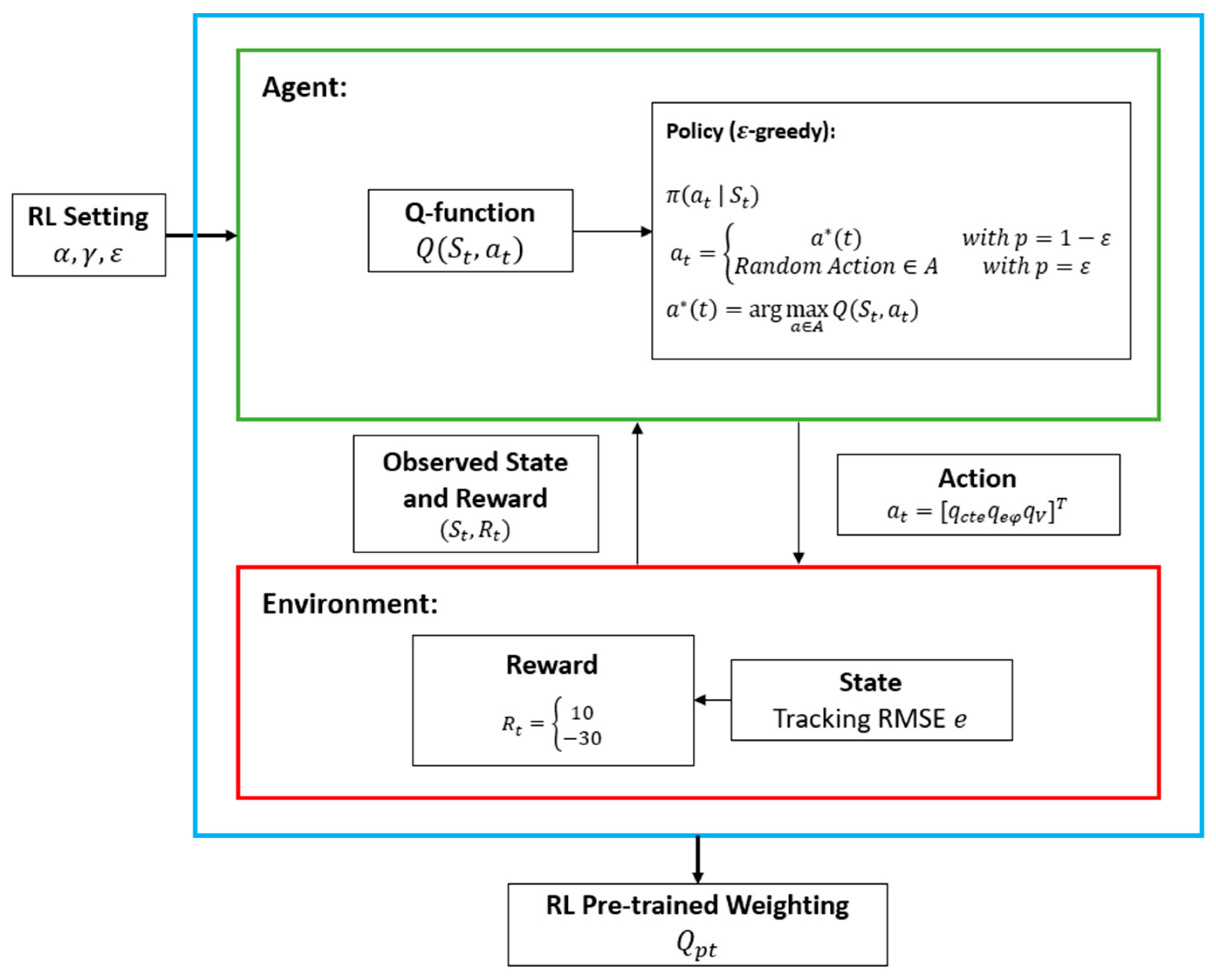
The concept of applying RL is simple, and a typical RL system is formed with the interaction of an agent and an environment. The RL training framework is shown in Figure 3, and is the policy that can determine which action could be applied according to the observed state . The reward function evaluates the rewards for the action applied to the RL. The agent is desired to react with the environment to obtain a higher reward by updating the policy.
is a component of the agent, and it updates in each iteration. By applying the Markov decision process (MDP) Equation (45), a Q-function can estimate the future state and reward of the system with the current state and action. As a consequence, the updated is indicated in Equation (46). The iteration process is further applied for the generation of optimal weighting of the RLMPC. The operation of the proposed RLMPC is to generate a datum value of , , and , and the rest of the parameters remain manually tuned to reduce the RL complexity. The definitions of state, action, and reward for the proposed RLMPC are shown in Equation (47). The relative RL setting is shown in Table 1, and , , and are denoted as the learning rate, greedy index, and discount rate, respectively.
Furthermore, the constraints of the control vector and control increments are designed by the Kronecker product in the form indicated in Equations (48) and (49).
According to the performance limitation of the proposed EV, the constraints applied in this paper are:
By combining Equations (41), (48) and (49), the optimized objective expression is defined in terms of applying the barrier interior point method (BIPM) with RL pretrained weighting matrices. After solving the QP problem in every time step, a series of control increments in the control horizon can be obtained, as shown in Equation (51).
The first element of the control series in Equation (51) is the actual input increment of the system, as indicated in Equation (52).
In the next time step, the system predicts a new output according to the state and undergoes the optimization process for new control increments. This procedure iterates until the whole path tracking mission is finished. As a consequence, the abovementioned RLMPC iteration process is summarized in Figure 4.
4. Simulations and Experiments
To evaluate the performance of the proposed vehicle positioning and path tracking methods, simulations and experiments on a full-scale, laboratory-made EV were arranged, and they are organized in three subsections.
4.1. Simulation of RLMPC-Based Path Tracking
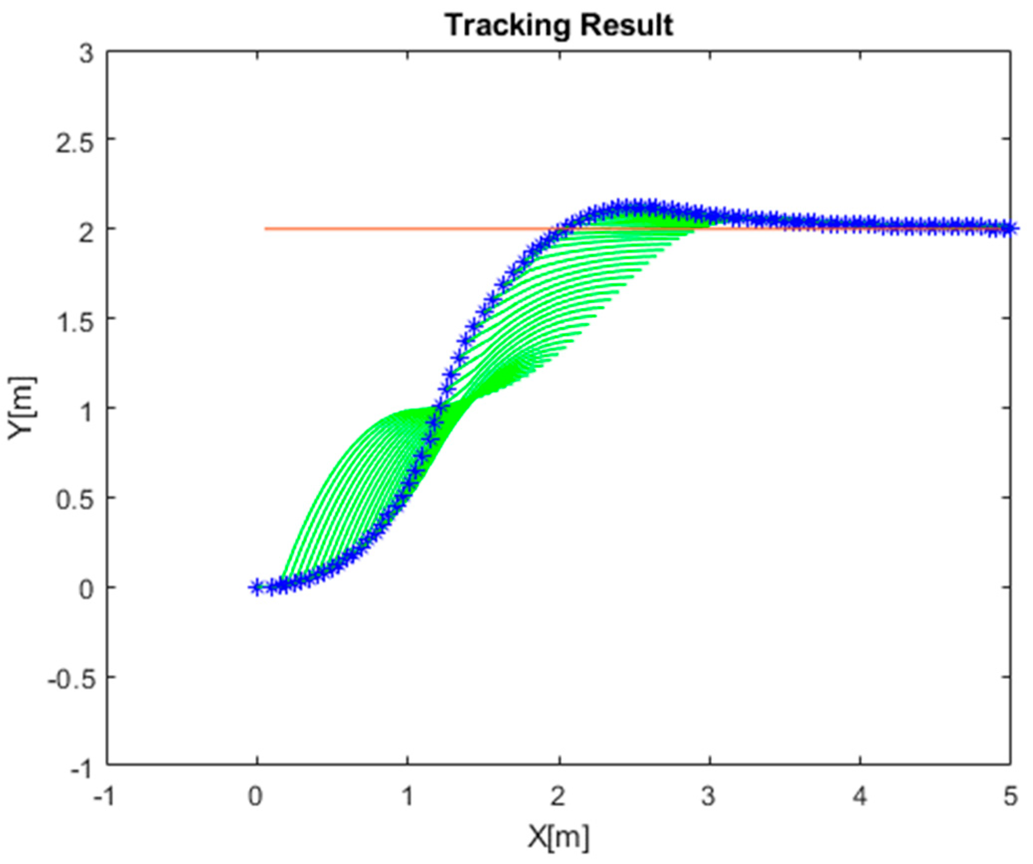
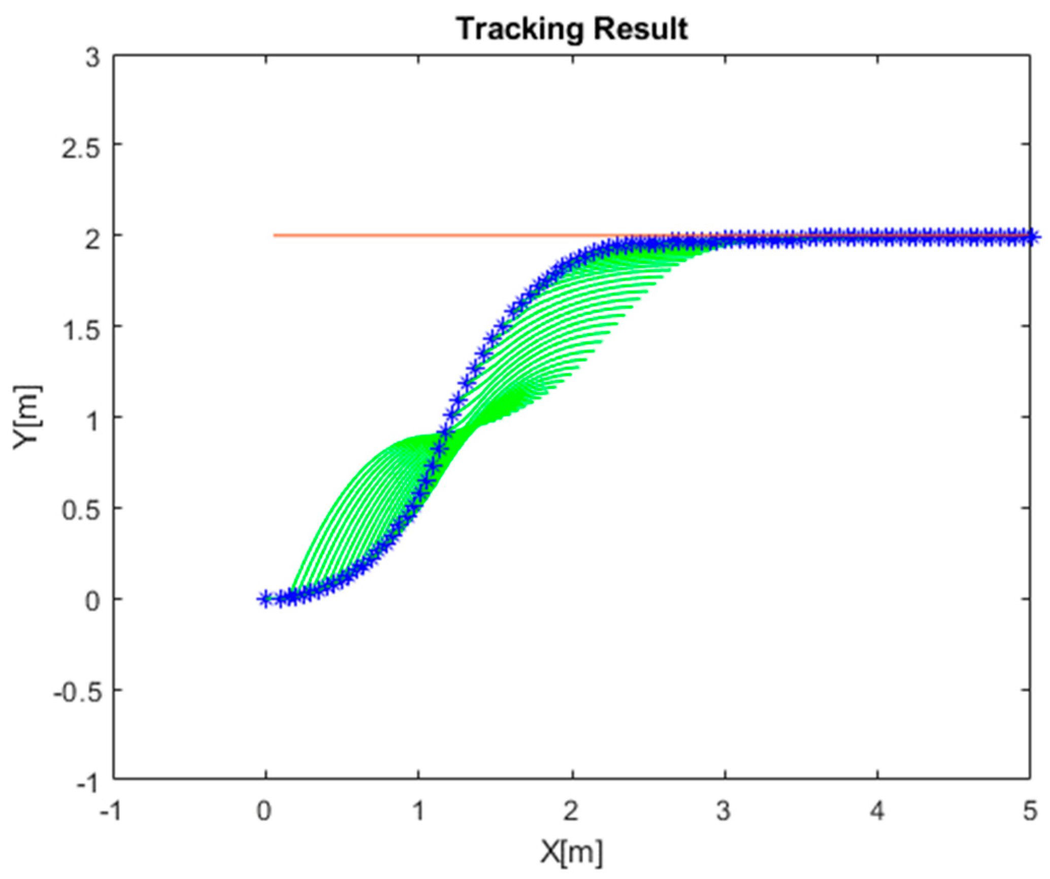
The simulations were arranged to evaluate the path tracking performance with respect to the manually tuned MPC and the RL-trained MPC methods. The trajectories of the abovementioned simulation results are shown in Figure 5 and Figure 6. It is noted that the green line represents the calculated path in every MPC iteration. The weighting matrices of the manually tuned MPC and the RL-trained MPC are indicated in Equations (53) and (54), respectively. The vehicle started from (0,0) with a heading of 0 rad, and it attempted to track the trajectory following a line path equation of y = 2. The manual parameter tuning took time, and the trajectory exhibited an overshoot at the desired line path. On the other hand, with the RL, a proper MPC parameter, indicated in Equation (54), was obtained without a time-consuming trial-and-error process. It was apparent that the RLMPC tracked the line path well without overshoots.
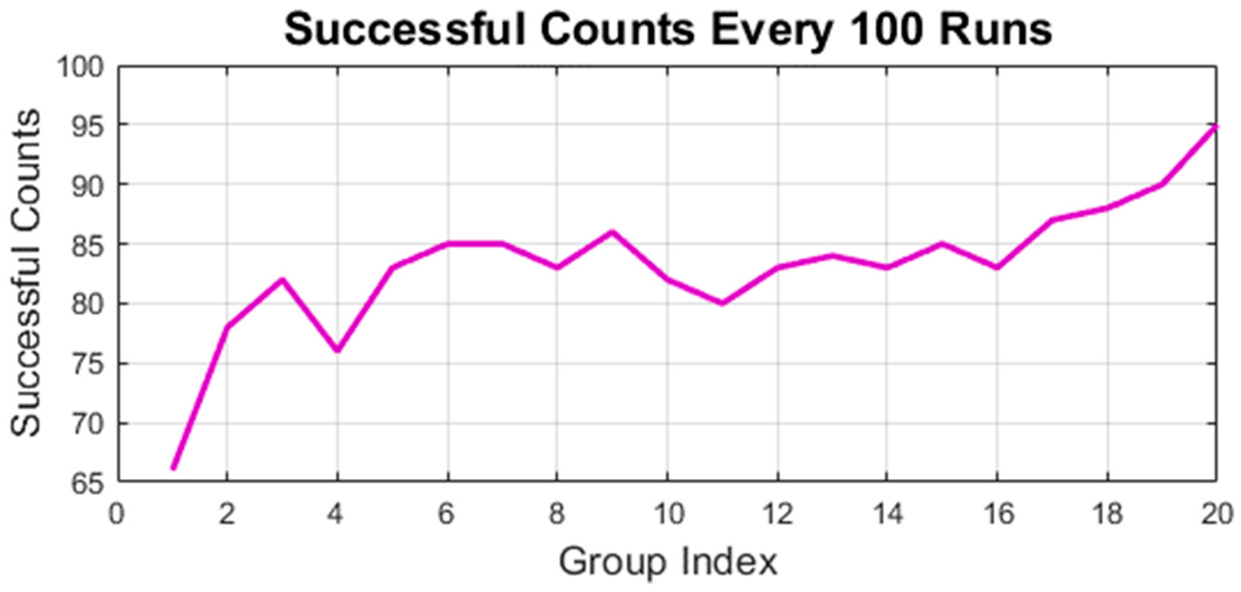
Finally, the RL performance is also indicated in Figure 7. As the learning iteration accumulated, the successful counts increased. Because there were only two states in this training procedure, this study raised the learning rate for fast convergence. The training result with the parameters shown in Table 1 is indicated in Equation (54).
4.2. Validation of Estimated Distance with Position Estimation
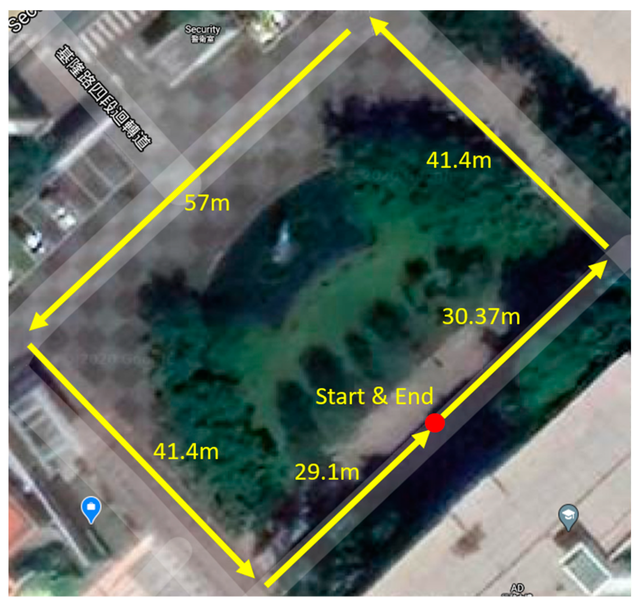
The second experiment was arranged to evaluate the UKF-based vehicle positioning system, and a rectangular path on the NTUST campus was arranged for validation, as shown in Figure 8. It is noted that, due to the campus driving speed and route limitation of the small campus of NTUST (90,000 m2), the following experiments were arranged simply. However, such a simple test environment was sufficient to examine the feasibility of integrating the aforementioned two technical aspects.
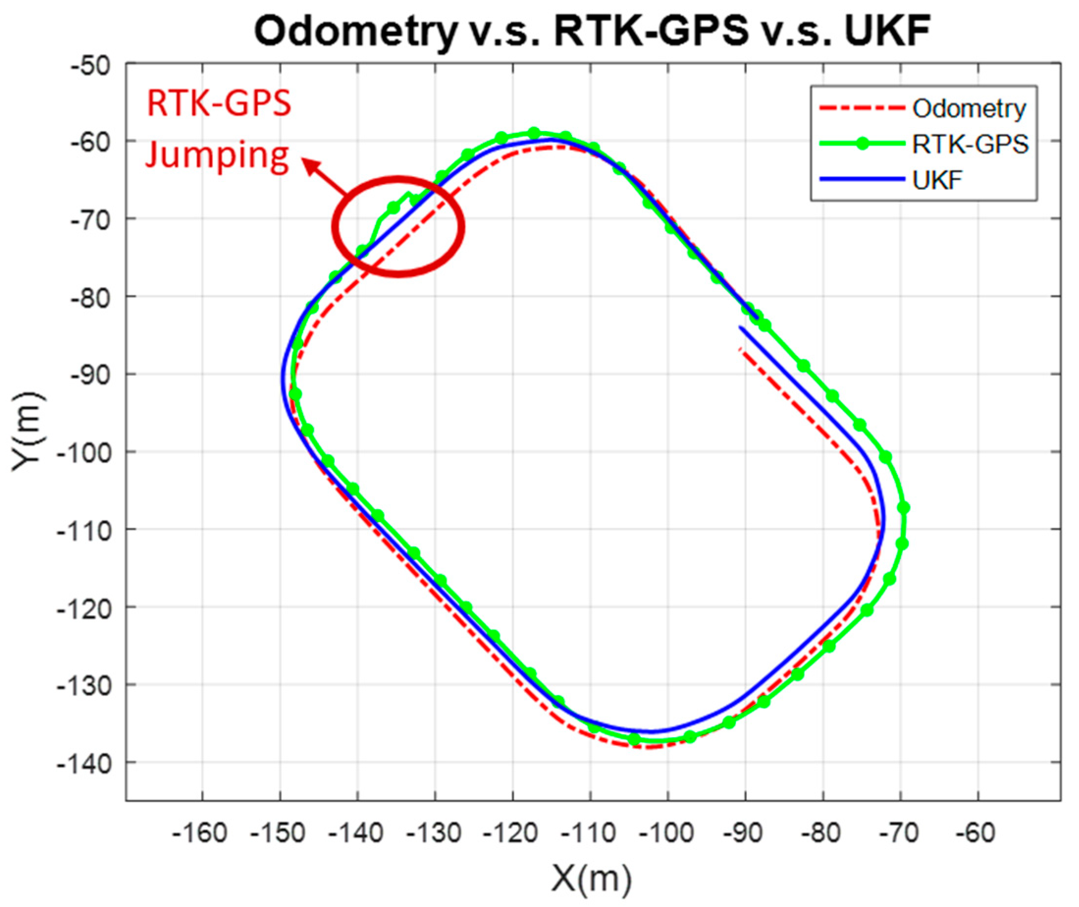
The RTK-GPS position obtained from the GGA instruction needed to be projected from the WGS84 system to the Cartesian coordinate system. Because the validation region in this paper was small, the equirectangular projection method was applied. The total distance of the rectangular path was approximately 199.37 m. The comparison of the traveling distance and the trajectory of odometry, RTK-GPS, and UKF are shown in Table 2 and Figure 9. Moreover, the comparison of odometry and the RTK and UKF methods are shown in Table 3.
The experimental results showed that the error of the UKF position estimator was 0.826%, as evaluated by the ground truth measured by the authors. Table 2 also indicates that the UKF represented the minimum error, mean error, and standard deviation when compared to odometry and RTK. Moreover, Table 3 shows a performance comparison with the state-of-the-art methods [10,14]. Our purpose was to know the performance of our UKF localization. We evaluated if the error percentage produced by the UKF was superior to other approaches. Although the experimental range and path were not the same, the proposed UKF demonstrated acceptable mean error and standard deviation.
Finally, Figure 9 shows the trajectory comparison of odometry and the RTK-GPS and UKF methods. It is also worth noting that on the top left of Figure 9 the RTK-GPS exhibits an outward jump. However, the UKF position estimator remained quite stable. The UKF position estimator also reduced the accumulative error that occurred when using odometry only.
4.3. Integrated Experiment with EV by Applying RL-Based MPC
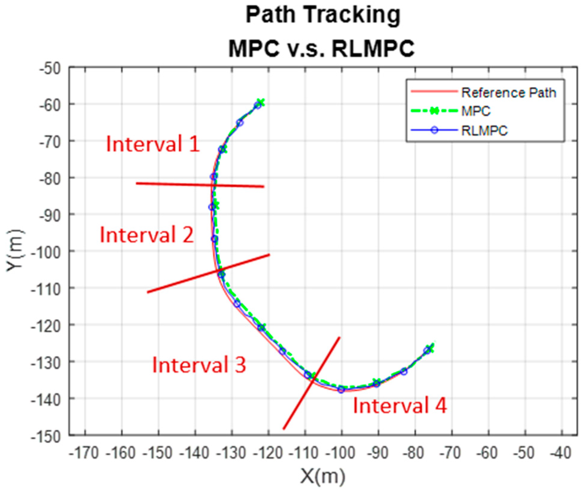
The path can be any combined planner equations. For example, the test scenario 2 was composed of four segments. The reference path was formed by recording the trajectory of manual driving. The recorded trajectory was manually processed in terms of driving as four segments, and each segment was further represented as an equation in terms of the curve fitting approach. Such combined equations are available to be tracked in terms of RL MPC.
In this experiment, an EV was used for trajectory tracking based on human-tuned and RLMPC control schemes. Two experimental scenarios were arranged on the NTUST campus: (1) a straight-line path and (2) a combinational path. It is noted that the straight-line path of scenario 1 is indicated as in Equation (55) and the combinational path of scenario 2 is indicated in Equation (56). For the combinational path in Equation (56), a smoothing spline was utilized to obtain a piecewise linear function with four intervals (i = 1 to 4). The weight was set as , and the corresponding smoothing parameter for each interval is indicated in Equation (57).
Mechanism tolerance, hardware limitations, and other factors might influence practical implementation. This work applied a pre-trained weighting matrix, shown in Equation (54), as the datum value of a full-scale EV experiment. Based on empirical knowledge and the pre-trained datum value of the weighting matrix, it can significantly reduce the parameter tuning time. The practical weighting matrices and were further revised for RLMPC, as indicated in Equation (58). The weighting matrices applied in non-RLMPC that were tuned by the operator were the same as the simulation case indicated in Equation (53).
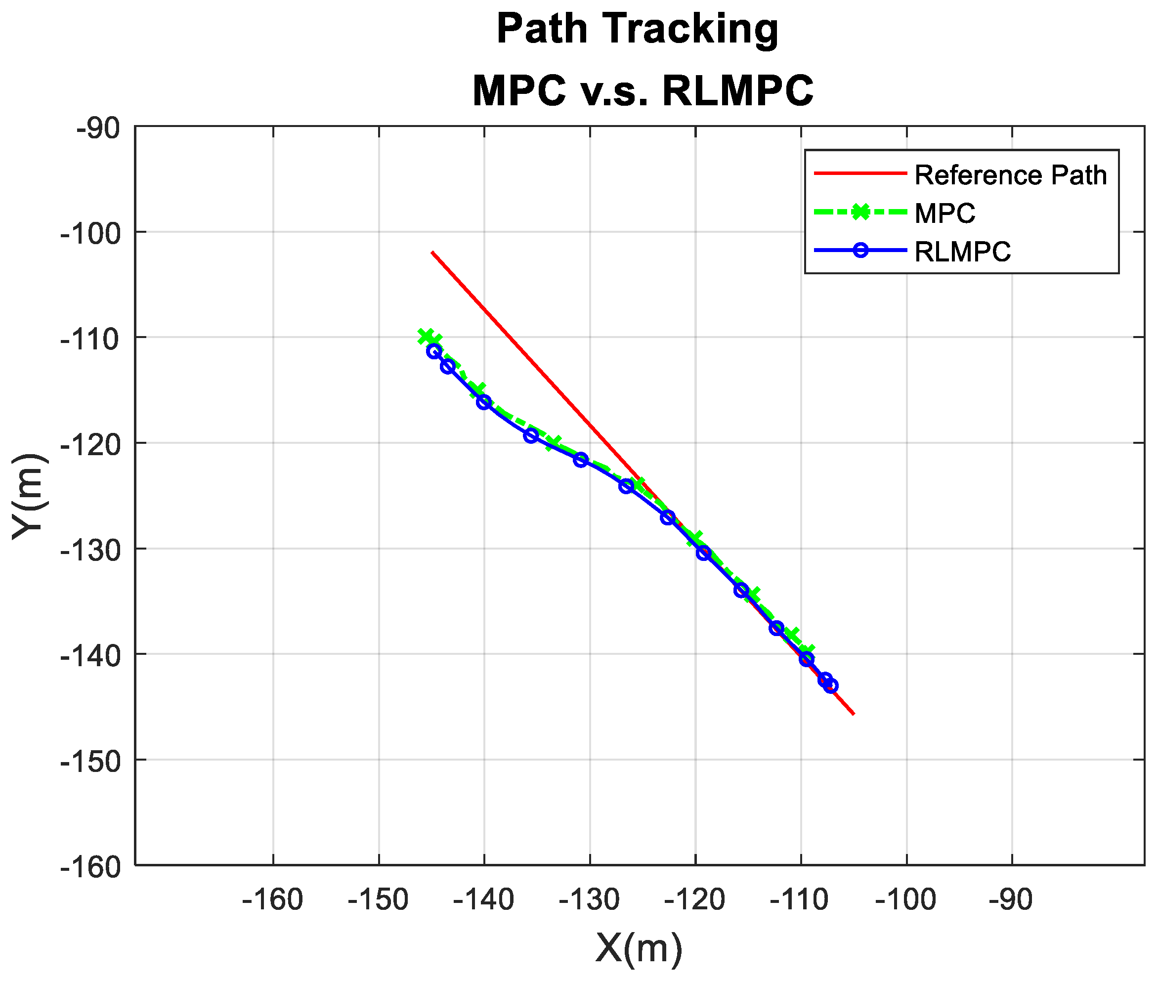
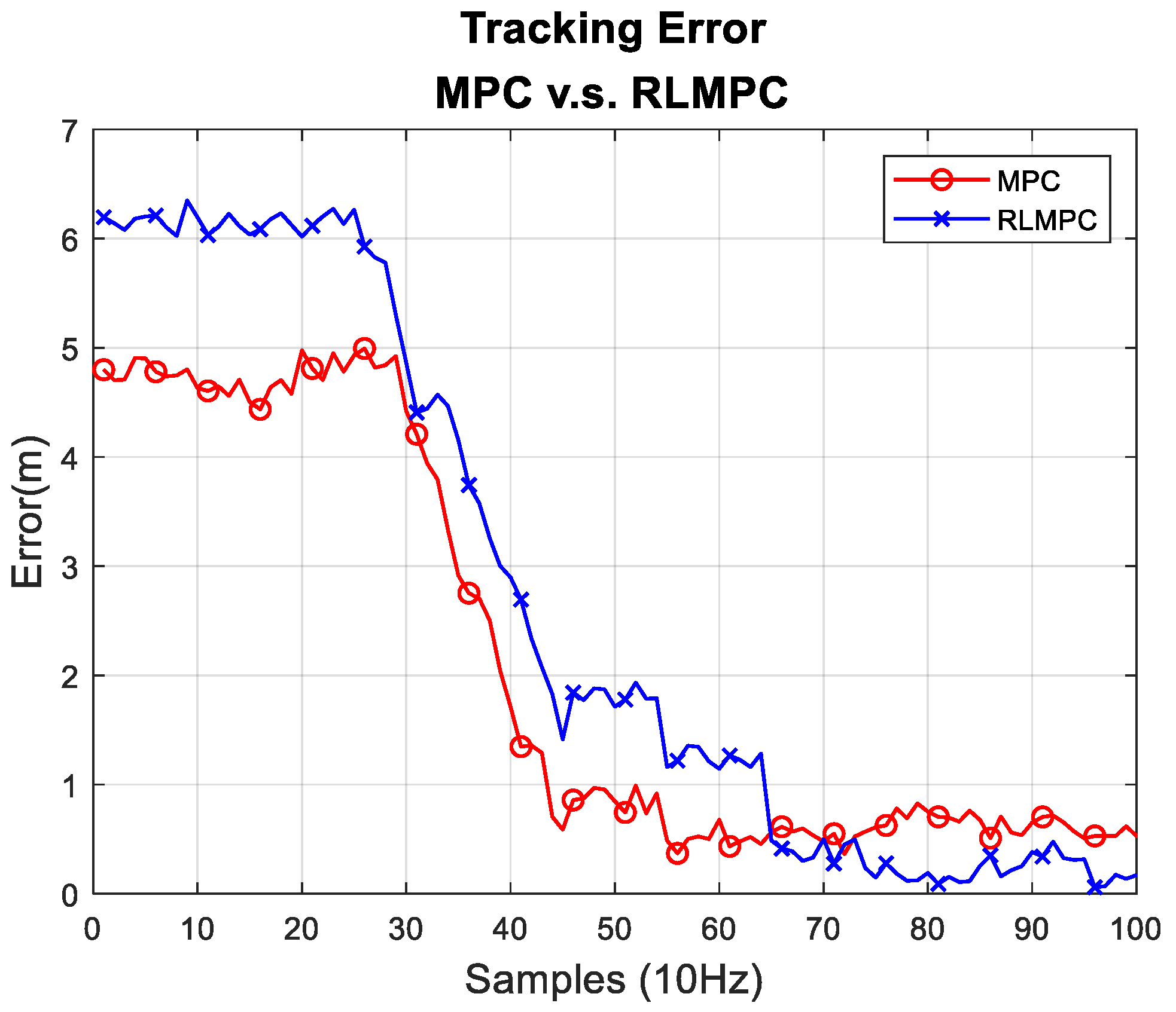
For scenario 1 experiments, the path tracking results of MPC and RLMPC are shown in Figure 10, and the tracking errors of MPC and RLMPC are indicated in Figure 11. The line path tracking results were quite similar to the aforementioned simulation results shown in Figure 5 and Figure 6. The human-tuned MPC represented some oscillation when the EV reached the line path. Nevertheless, the RLMPC exhibited a smaller error after the 70th sample.
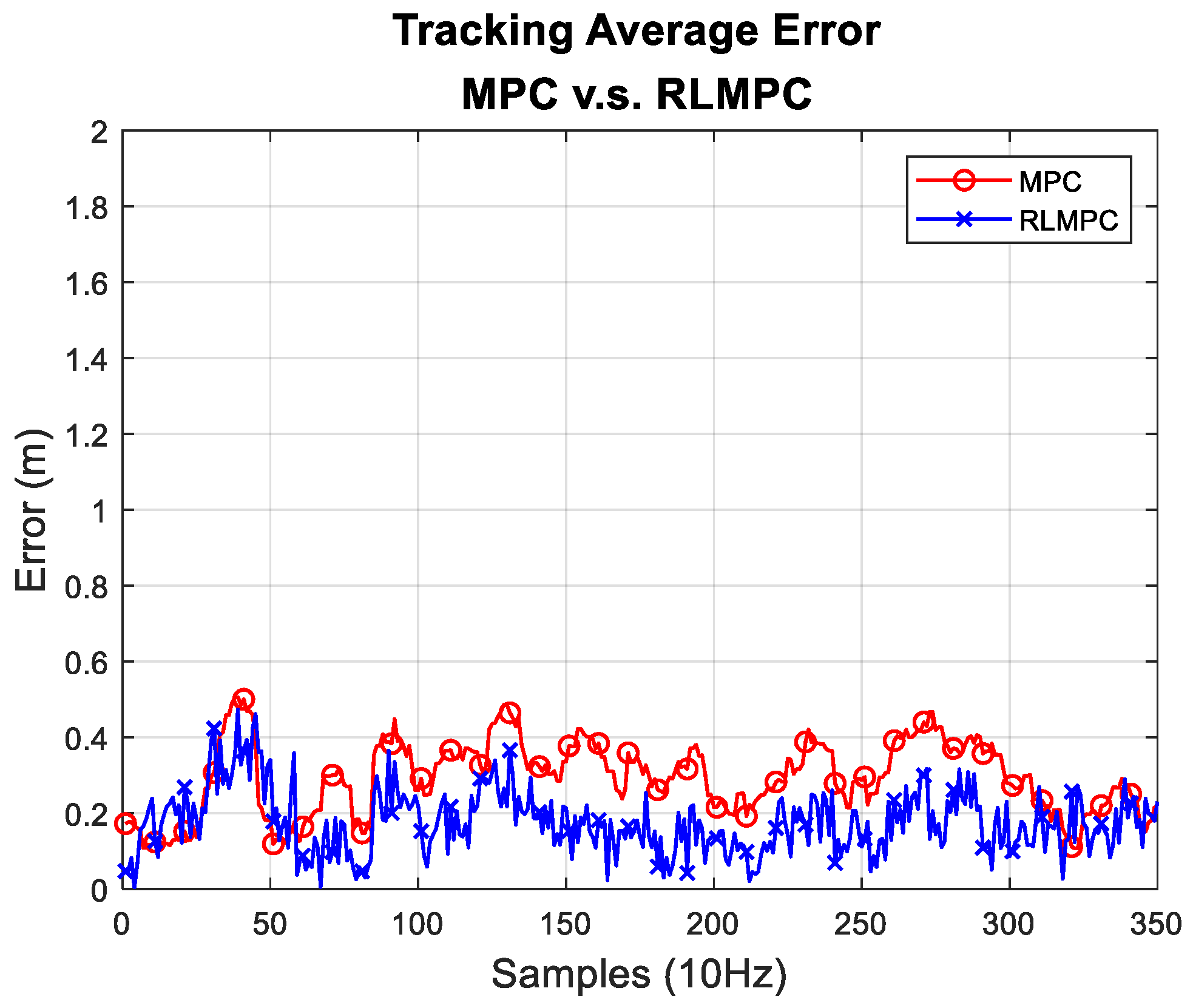
For the scenario 2 experiments, the path tracking results of MPC and RLMPC are shown in Figure 12, and the tracking errors of MPC and RLMPC are indicated in Figure 13. It was apparent that the RLMPC outperformed the tracking error compared to the human-tuned MPC. To provide a confident and quantitative error evaluation, all the experiments were performed three times for the performance comparison, as indicated in Table 4. Table 4 shows the relative statistical data of averaging the values of the three trials. Both of the average RMSEs were less than 0.3 m, and the maximum errors were less than 0.7 m. The overall results showed that the RLMPC and human-tuned MPC followed the same trajectory well. However, with well-converged parameters, RLMPC had better performance than MPC tuned by humans in terms of maximum error, average error, standard deviation, and RMSE.
5. Conclusions and Future Works
In this paper, a reinforcement learning-based MPC framework is presented. The proposed RLMPC significantly reduced the efforts of tuning MPC parameters. The RLMPC executed with the UKF-based vehicle positioning system that considered the RTK, odometry, and IMU sensor data. The proposed UKF vehicle positioning and RLMPC path tracking methods were validated with a full-scale, laboratory-made EV on the NTUST campus. On a 199.27 m loop path, the UKF estimated travel distance error was 0.82%. The MPC parameters generated by RL achieved an RMSE of 0.227 m in the path tracking experiments, and it also exhibited better tracking performance than the human-tuned MPC parameters.
Moreover, the aim of this work was to integrate two important practices of realizing an autonomous vehicle in a campus environment, including vehicle positioning and path tracking. Such a project is helpful to students in university to easily reach, learn, and practice key technologies of autonomous vehicles. As a consequence, this work was not aiming at providing significant improvement on the localization accuracy or RL MPC performance. Hence, the future works on the localization accuracy and RL MPC performance in terms of two independent projects will be studied based on the laboratory-made electric vehicle and the preliminary localization and path tracking results. For example, the use of robust MPC based on safe reinforcement learning [31] would be an important direction to improve the path tracking performance. Moreover, due to the campus driving speed and route limitation of the small campus of NTUST (90,000 m2), this paper just showed the preliminary results on the successful integration of vehicle localization and path tracking. Moving the vehicle to a more complicated test environment would be another important future work.
On the other hand, obstacle avoidance was not a purpose of this work. The 360° scan formed with two lidar devices temporarily stopped the driving of EVs during path tracking when any obstacles were detected to ensure safety. In the future, an effective reactive obstacle avoidance approach will be further considered to improve autonomous driving efficiency in a dynamic obstacle environment. Moreover, the proposed UKF can further combine 3D-LiDar and visual SLAM to improve the vehicle positioning robustness. On the other hand, only three components in were considered for RL in this paper. In the future, all parameters in this matrix will be considered and evaluated.
Author Contributions
J.-A.Y. was responsible for hypothoses, system deployment, experiments, and paper draft writing; C.-H.K. is the advisor who oriented the research direction for the paper and gave comments and advice to do this research. All authors have read and agreed to the published version of the manuscript.
Funding
Ministry of Science and Technology, Taiwan under Grant MOST 109-2221-E-011-112-MY3 and the “Center for Cyber-physical System Innovation” from The Featured Areas Research Center Program within the framework of the Higher Education Sprout Project by the Ministry of Education (MOE) in Taiwan.
Conflicts of Interest
The authors declare no conflict of interest.
References
- Wan, E.A.; Van Der Merwe, R. The unscented Kalman filter for nonlinear estimation. In Proceedings of the IEEE 2000 Adaptive Systems for Signal Processing, Communications, and Control Symposium (Cat. No.00EX373), Lake Louise, AB, Canada, 4 October 2000; pp. 153–158. [Google Scholar]
- Rose, C.; Britt, J.; Allen, J.; Bevly, D.M. An Integrated Vehicle Navigation System Utilizing Lane-Detection and Lateral Position Estimation Systems in Difficult Environments for GPS. IEEE Trans. Intell. Transp. Syst. 2014, 15, 2615–2629. [Google Scholar] [CrossRef]
- Um, I.; Park, S.; Oh, S.; Kim, H. Analyzing Location Accuracy of Unmanned Vehicle According to RTCM Message Frequency of RTK-GPS. In Proceedings of the 2019 25th Asia-Pacific Conference on Communications (APCC), Ho Chi Minh City, Vietnam, 6–8 November 2019; pp. 326–330. [Google Scholar]
- Kim, J.W.; Lee, D.K.; Bin Cao, S.; Lee, S.S. Availability evaluation and development of network-RTK for vehicle in downtown. In Proceedings of the 2014 International Conference on Information and Communication Technology Convergence (ICTC), Busan, Korea, 22–24 October 2014; pp. 557–558. [Google Scholar]
- Liu, T.; Li, B. Single-frequency BDS/GPS RTK with low-cost U-blox receivers. In Proceedings of the 2017 Forum on Cooperative Positioning and Service (CPGPS), Harbin, China, 19–21 May 2017; pp. 232–238. [Google Scholar]
- Ng, K.M.; Johari, J.; Abdullah, S.A.C.; Ahmad, A.; Laja, B.N. Performance Evaluation of the RTK-GNSS Navigating under Different Landscape. In Proceedings of the 2018 18th International Conference on Control, Automation and Systems (ICCAS), PyeongChang, Korea, 17–20 October 2018; pp. 1424–1428. [Google Scholar]
- Um, I.; Park, S.; Kim, H.T.; Kim, H. Configuring RTK-GPS Architecture for System Redundancy in Multi-Drone Operations. IEEE Access 2020, 8, 76228–76242. [Google Scholar] [CrossRef]
- Maier, D.; Kleiner, A. Improved GPS sensor model for mobile robots in urban terrain. In Proceedings of the 2010 IEEE International Conference on Robotics and Automation, Anchorage, AK, USA, 3–7 May 2010; pp. 4385–4390. [Google Scholar]
- Yi, S.; Worrall, S.; Nebot, E. Geographical Map Registration and Fusion of Lidar-Aerial Orthoimagery in GIS. In Proceedings of the 2019 IEEE Intelligent Transportation Systems Conference (ITSC), Auckland, New Zealand, 27–30 October 2019; pp. 128–134. [Google Scholar]
- Wei, L.; Cappelle, C.; Ruichek, Y.; Zann, F. Intelligent Vehicle Localization in Urban Environments Using EKF-based Visual Odometry and GPS Fusion. IFAC Proc. Vol. 2011, 44, 13776–13781. [Google Scholar] [CrossRef] [Green Version]
- Aftatah, M.; Lahrech, A.; Abounada, A. Fusion of GPS/INS/Odometer measurements for land vehicle navigation with GPS outage. In Proceedings of the 2016 2nd International Conference on Cloud Computing Technologies and Applications (CloudTech), Marrakech, Morocco, 24–26 May 2016; pp. 48–55. [Google Scholar] [CrossRef]
- Henkel, P.; Sperl, A.; Mittmann, U.; Bensch, R.; Farber, P. Precise Positioning of Robots with Fusion of GNSS, INS, Odometry, LPS and Vision. In Proceedings of the 2019 IEEE Aerospace Conference, Big Sky, MT, USA, 2–9 March 2019; pp. 1–6. [Google Scholar]
- Mohamed, S.A.S.; Haghbayan, M.-H.; Westerlund, T.; Heikkonen, J.; Tenhunen, H.; Plosila, J. A Survey on Odometry for Autonomous Navigation Systems. IEEE Access 2019, 7, 97466–97486. [Google Scholar] [CrossRef]
- Mikov, A.; Panyov, A.; Kosyanchuk, V.; Prikhodko, I. Sensor Fusion for Land Vehicle Localization Using Inertial MEMS and Odometry. In Proceedings of the 2019 IEEE International Symposium on Inertial Sensors and Systems (INERTIAL), Naples, FL, USA, 1–5 April 2019; pp. 1–2. [Google Scholar] [CrossRef]
- Zhao, S.; Chen, Y.; Farrell, J.A. High-Precision Vehicle Navigation in Urban Environments Using an MEM’s IMU and Single-Frequency GPS Receiver. IEEE Trans. Intell. Transp. Syst. 2016, 17, 2854–2867. [Google Scholar] [CrossRef]
- Chen, M.; Ren, Y. MPC based path tracking control for autonomous vehicle with multi-constraints. In Proceedings of the 2017 International Conference on Advanced Mechatronic Systems (ICAMechS), Xiamen, China, 6–9 December 2017; pp. 477–482. [Google Scholar]
- Paden, B.; Cap, M.; Yong, S.Z.; Yershov, D.; Frazzoli, E. A Survey of Motion Planning and Control Techniques for Self-Driving Urban Vehicles. IEEE Trans. Intell. Veh. 2016, 1, 33–55. [Google Scholar] [CrossRef] [Green Version]
- Jhang, J.-H.; Lian, F.-L. An Autonomous Parking System of Optimally Integrating Bidirectional Rapidly-Exploring Random Trees* and Parking-Oriented Model Predictive Control. IEEE Access 2020, 8, 163502–163523. [Google Scholar] [CrossRef]
- Shen, C.; Guo, H.; Liu, F.; Chen, H. MPC-based path tracking controller design for autonomous ground vehicles. In Proceedings of the 2017 36th Chinese Control Conference (CCC), Dalian, China, 26–28 July 2017; pp. 9584–9589. [Google Scholar]
- Tang, W.; Yang, M.; Wang, C.; Wang, B.; Zhang, L.; Le, F. MPC-Based Path Planning for Lane Changing in Highway Environment. In Proceedings of the 2018 Chinese Automation Congress (CAC), Xi’an, China, 30 November–2 December 2018; pp. 1003–1008. [Google Scholar]
- Chen, Y.; Wang, J. Trajectory Tracking Control for Autonomous Vehicles in Different Cut-in Scenarios. In Proceedings of the 2019 American Control Conference (ACC), Philadelphia, PA, USA, 10–12 July 2019; pp. 4878–4883. [Google Scholar]
- Dixit, S.; Montanaro, U.; Dianati, M.; Oxtoby, D.; Mizutani, T.; Mouzakitis, A.; Fallah, S. Trajectory Planning for Autonomous High-Speed Overtaking in Structured Environments Using Robust MPC. IEEE Trans. Intell. Transp. Syst. 2020, 21, 2310–2323. [Google Scholar] [CrossRef]
- Liniger, A.; Domahidi, A.; Morari, M. Optimization-based autonomous racing of 1:43 scale RC cars. Optim. Control Appl. Methods 2015, 36, 628–647. [Google Scholar] [CrossRef] [Green Version]
- Rosolia, U.; Carvalho, A.; Borrelli, F. Autonomous racing using learning Model Predictive Control. In Proceedings of the 2017 American Control Conference (ACC), Seattle, WA, USA, 24–26 May 2017; pp. 5115–5120. [Google Scholar]
- Lin, F.; Chen, Y.; Zhao, Y.; Wang, S. Path tracking of autonomous vehicle based on adaptive model predictive control. Int. J. Adv. Robot. Syst. 2019, 16, 1–12. [Google Scholar] [CrossRef]
- Görges, D. Relations between Model Predictive Control and Reinforcement Learning. IFAC-PapersOnLine 2017, 50, 4920–4928. [Google Scholar] [CrossRef]
- Xie, H.; Xu, X.; Li, Y.; Hong, W.; Shi, J. Model Predictive Control Guided Reinforcement Learning Control Scheme. In Proceedings of the 2020 International Joint Conference on Neural Networks (IJCNN), Glasgow, UK, 19–24 July 2020; pp. 1–8. [Google Scholar]
- Guan, Y.; Ren, Y.; Li, S.E.; Sun, Q.; Luo, L.; Li, K. Centralized Cooperation for Connected and Automated Vehicles at Intersections by Proximal Policy Optimization. IEEE Trans. Veh. Technol. 2020, 69, 12597–12608. [Google Scholar] [CrossRef]
- Tange, Y.; Kiryu, S.; Matsui, T. Model Predictive Control Based on Deep Reinforcement Learning Method with Discrete-Valued Input. In Proceedings of the 2019 IEEE Conference on Control Technology and Applications (CCTA), Hong Kong, China, 19–21 August 2019. [Google Scholar]
- Modalavalasa, H.K.; Makkena, M.L. Intelligent Parameter Tuning Using Segmented Adaptive Reinforcement Learning Algorithm. In Proceedings of the 2020 International Conference on Electronics and Sustainable Communication Systems (ICESC), Coimbatore, India, 2–4 July 2020; pp. 252–256. [Google Scholar]
- Zanon, M.; Gros, S. Safe Reinforcement Learning Using Robust MPC. IEEE Trans. Autom. Control 2021, 66, 3638–3652. [Google Scholar] [CrossRef]
Figure 1.
Overall operation flowchart.

Figure 2.
A laboratory-made EV for experiments in this paper (left-hand-side); the kinematic bicycle model for illustrating the kinematics (right-hand-side).
Figure 2.
A laboratory-made EV for experiments in this paper (left-hand-side); the kinematic bicycle model for illustrating the kinematics (right-hand-side).

Figure 3.
Proposed RL framework.

Figure 4.
Proposed RL-based MPC (RLMPC) training framework.

Figure 5.
Line path tracking with manually tuned MPC parameters.

Figure 6.
Line path tracking with RL-trained MPC parameters.

Figure 7.
RL learning performance.

Figure 8.
A rectangular path on the NTUST campus for vehicle positioning validation.

Figure 9.
Trajectory comparison of odometry, RTK, and UKF.

Figure 10.
Trajectory comparison of MPC and RLMPC in scenario 1.

Figure 11.
Tracking error comparison of MPC and RLMPC in Scenario 1.

Figure 12.
Trajectory comparison of MPC and RLMPC in scenario 2.

Figure 13.
Tracking error comparison of MPC and RLMPC in Scenario 2.


Table 1.
RL Parameter Setting.
| α-Parameter | ε-Parameter | γ-Parameter | Training Episodes |
|---|---|---|---|
| 0.5 | 0.2 | 0.95 | 2000 |
Table 2.
Comparison of Travel Distances Using Odometry, RTKGPS, and UKF.
| Methods | Ground Truth (m) | Estimated Distance (m) | Error (%) | Mean Error (m) | Standard Deviation (m) |
|---|---|---|---|---|---|
| Odometry | 199.27 | 192.882 | 3.205 | 6.387 | 4.856 |
| RTKGPS | 199.27 | 197.462 | 1.684 | 3.356 | 2.243 |
| UKF | 199.27 | 198.201 | 0.826 | 1.646 | 1.198 |
| Proposed Method | Wei [10] | Mikov [14] | |
|---|---|---|---|
| Ground Truth (m) | 199.27 | 674.5 | 10,352 ± 3749 |
| Estimated Distance (m) | 198.201 | 683.18 | 10,404 ± 3777 |
| Error (%) | 0.826 | 1.29 | 0.502 ± 0.746 |
| Mean Error (m) | 1.646 | 1.23 | - |
| Standard Deviation (m) | 1.198 | 1.05 | 28 |
Table 4.
Comparison of Path Tracking Performance of Scenario 2.
| Method | Maximum Error (m) | Average Error (m) | Standard Deviation (m) | RMSE (m) |
|---|---|---|---|---|
| MPC | 0.671 | 0.291 | 0.138 | 0.257 |
| RLMPC | 0.615 | 0.196 | 0.112 | 0.227 |
Publisher’s Note: MDPI stays neutral with regard to jurisdictional claims in published maps and institutional affiliations. |
© 2021 by the authors. Licensee MDPI, Basel, Switzerland. This article is an open access article distributed under the terms and conditions of the Creative Commons Attribution (CC BY) license (https://creativecommons.org/licenses/by/4.0/).
Share and Cite
MDPI and ACS Style
Yang, J.-A.; Kuo, C.-H. Integrating Vehicle Positioning and Path Tracking Practices for an Autonomous Vehicle Prototype in Campus Environment. Electronics 2021, 10, 2703. https://0-doi-org.brum.beds.ac.uk/10.3390/electronics10212703
AMA Style
Yang J-A, Kuo C-H. Integrating Vehicle Positioning and Path Tracking Practices for an Autonomous Vehicle Prototype in Campus Environment. Electronics. 2021; 10(21):2703. https://0-doi-org.brum.beds.ac.uk/10.3390/electronics10212703
Chicago/Turabian StyleYang, Jui-An, and Chung-Hsien Kuo. 2021. "Integrating Vehicle Positioning and Path Tracking Practices for an Autonomous Vehicle Prototype in Campus Environment" Electronics 10, no. 21: 2703. https://0-doi-org.brum.beds.ac.uk/10.3390/electronics10212703
Note that from the first issue of 2016, this journal uses article numbers instead of page numbers. See further details here.