Radar Angle of Arrival System Design Optimization Using a Genetic Algorithm

Abstract

An approach for using a Genetic Algorithm (GA) to select radar design parameters related to beamforming and angle of arrival estimation is presented in this article. This was accomplished by first developing a simulator that could evaluate the localization performance with a given set of design parameters. The simulator output was utilized as part of the GA objective function that searched the solution space for an optimal set of design parameters. Using this approach, the authors were able to more than halve the mean squared error in degrees of the localization algorithm versus a radar design using human-selected design parameters. The results of this study indicate that this kind of approach can be used to aid in the development of an actual radar design.

1. Introduction

Genetic Algorithms (GAs) are biologically-inspired solutions used for problems where the proposed solutions can be encoded in a population. The GA uses a genetics-based approach to examine the solution space. Herein, a GA is utilized to search over the combination of the number of receive elements in an array, element locations (and therefore, element spacings) and element weightings to minimize the Angle Of Arrival (AOA) error over the receive field of view.

The main contribution of this work is the development of a GA program for automating the selection of several radar design parameters related to beamforming and localization. The proposed GA is able to search over a large design space, which includes parameters for controlling the number of transmit and receive elements, the element spacing, the number of steered beams for receive beamforming, the steering angles for beamforming, transmit and receive array weightings. The system optimizes these parameters subject to user-defined constraints in order to minimize the receive angle of arrival mean square error (MSE). To the best of our knowledge, this is the first time a GA has been used for a radar system design.

This paper is organized as follows. Section 2 briefly discusses the background of beamforming, angle of arrival estimation and genetic algorithms. Section 3 discusses the methodology used and the proposed GA solution. Section 4 examines the results of the various experiments. Section 5 draws conclusions, and Section 6 discusses potential future work.

2. Background

In this section, an overview of Particle Swarm Optimization (PSO), Invasive Weed Optimization (IWO) and GAs is given in Section 2.1.1, Section 2.1.2 and Section 2.1.3, respectively. Applications of PSO, IWO and GA in radar are listed in Section 2.2. A short background in beamforming and Angle Of Arrival (AOA) estimation is given in Section 2.3 and Section 2.4, respectively.

2.1. Optimization Methods

There are many optimization techniques used in radar processing and design. Classic optimization approaches include techniques such as constrained optimization [1], least squares optimization and numerical optimizations based on sidelobe control for monopulse antennas (e.g., Taylor and Bayliss tapers), and many others.

Nature-inspired optimization techniques include GA, PSO, IWO and others. These methods are overviewed in the following sections.

2.1.1. Particle Swarm Optimization Overview

In PSO, candidate solutions are modeled as particles with position and velocity components. The position represents the current set of values in the N-dimensional solution space. Each particle is evaluated to generate a score. The velocity component controls where the particle goes and is set based on a combination of the local best score achieved by that particle and the best score achieved by any particle. After some number of iterations, the solution is the best score found.

The PSO can draw other particles when one discovers a good solution (the so-called cognitive and social influence). There are several limitations to PSO optimization that may affect PSO problem solving [2]. These limitations are related to the sensitivity of search to transformations (rotation, translation and scale), local convergence, stability, first hitting time and biases [2]. Improper accelerations and inertia weights can cause particles to accelerate uncontrollably. This is remedied by placing convergence boundary constraints. Many PSOs are also sensitive to non-separability (rotation variance) in the search space [3].

A good overview of PSO can be found in [4]. Poli et al. [5] concluded that PSOs are popular with practitioners because they are simple, fairly easily extended into new problem domains, reliable and usually deliver good results (though not necessarily the best results.)

2.1.2. Invasive Weeds Optimization Overview

The IWO was developed by Mehrabian, Reza and Caro [6], based on the robust nature of weeds (anyone who owns property can attest to the veracity of weeds). The basic idea for IWO is that a finite number of seeds is initially dispersed over the search area. Each seed grows to a flowering plant and produces seeds depending on its fitness, which are randomly dispersed over the search area and grow into new plants, giving some spatial diversity. Once a maximum number of plants is reached, then the survival of the fittest is enforced. The process continues until maximum iterations are reached. Again, there is no guarantee that the best solution will be found. However, in practice, usually very good solutions are found.

2.1.3. Genetic Algorithm Overview

GAs are basically searching and optimization algorithms and are part of a class of machine learning called evolutionary computation [7,8]. GAs have a pool of possible solutions encoded in the genes, and they have rules, usually based on probability, to search the space. They also have a fitness function, which is maximized (or minimized).

GAs in general do not require gradient or derivative information, can search a large space and can provide a list of good solutions. They do have some well-known limitations. They are not guaranteed to converge to the optimal solution, and each epoch requires many calculations of the fitness function, which may be computationally expensive. However, they can usually provide a “near-optimal” solution in a reasonable amount of time.

In a GA implementation, there is a population made up of multiple chromosomes. Each chromosome contains many genes, which encode information about the solution. A fitness function evaluates the fitness of the solutions. There are basic operations, such as crossover, mutation, etc., that allow the population to change over time and inherit characteristics from other chromosomes. Usually as part of the GA, there is a probability that these operations will occur. Crossover is where one or more genes (characteristics or parameters) are swapped. Mutation is where a gene’s encoding is randomly changed. Crossover allows the GA to move good characteristics around as generations progress. Mutation allows the GA to expand the search space. Selection is another operation in the GA. In roulette wheel selection, one method is to make the probability of selection proportional to the fitness function, essentially assigning a fractional probability based on the how good a given fitness score is versus the sum of the fitness scores of the rest of the population. Linear and non-linear Rank algorithms are also sometimes used with roulette selection. These algorithms sort the fitness scores of the population and assign fixed probabilities based on where they fall in the sort order. These approaches are useful to ensure that even poorly-performing chromosomes still have a chance to reproduce.

The GA is a search optimization tool. Given some objective function, it will search for possible solutions to a problem that come as close as possible to your objective. The GA is inspired by nature and is based on the biological aspect of reproduction and survival of the fittest. This genetic modeling of the problem with a population of possible solutions that produces subsequent generations of solutions can eventually arrive at a highly optimized result. GAs are very flexible in that they can handle highly non-linear systems and generally are not constrained by the type of problem they are trying to solve (although the there may be constraints on the solutions they produce). This allows them to work pretty well for a wide range of problems.

The genetic algorithm itself is highly customizable, and numerous approaches for the different algorithm components have been developed over the years. These approaches include algorithms for initialization, selection, crossover, mutation and termination. One of the most important aspects of the GA is the objective function, which is used to evaluate how well a particular solution performs. This function is unique to the problem being solved, because it is in effect the definition of the problem. While it is possible to treat a GA as a black box and use whatever the default algorithms are, the objective function must be defined by the user. This is reflected in many of the articles presented here where a large amount of detail was given for the objective function, but much less was provided for how the rest of the GA was configured. Other more advanced options such as elitism and hall of fame ensure that the best solutions found during the progression of the algorithm persist until the end.

As a local optimization tool, the genetic algorithm has been utilized in large variety of applications. In architectural design, GAs have been applied to evaluate and predict the energy consumption of designs [9] and optimize designs with regards to energy rating [10]. GAs have been used in molecular modeling to understand receptor sites to improve drug design [11] and to determine the structure of an atomic cluster, which has the lowest energy [12]. GAs have even been applied to their biological inspiration to analyze phylogenetic trees [13].

In general, PSO, GA and IWO are all heuristically-guided random search methods, and none of them are guaranteed to reach the optimal solution to a given problem. In practice, they all perform well in most cases. Hassan et al. studied GA and PSO for several problems and concluded that both obtain high-quality solutions, but in general, the PSO can reach these solutions quicker [14]. For offline design optimization (the subject of this paper), this is not an issue. In this work, we propose a GA to design a radar receive system by jointly optimizing the receiver element locations (spacings), the receive weightings in order to provide the lowest MSE for detecting the AOA.

2.2. Optimizations Used in Radar

This section discusses PSO, IWO and GA optimizations used in radar.

2.2.1. PSO Used in Radar

PSO has been previously used as an adaptive beamforming technique in phased arrays where the antenna element weights were set to achieve some objective, such as steering the main lobe to a particular signal of interest and creating nulls in the direction of interference. Examples of this can be found in [15], where an adaptive Neural Network (NN) beamformer is trained using a Mutated Boolean PSO (MBPSO). The beamformer is compared favorably to the Minimum Variance Distortionless Response (MVDR) beamformer. In [16], Zaharis et al. developed a PSO variant called Adaptive Mutated Boolean PSO (AMBPSO) using an efficient Boolean adaptive mutation process. AMBPSO estimates the excitation weights applied on the array elements considering that a desired signal and several interference signals are received by the array.

2.2.2. IWO Used in Radar

Zaharis et al. [17] utilized a modified version of IWO denoted Adaptive Dispersion Invasive Weed Optimization (ADIWO) where the seeds are dispersed with a standard deviation, which is a function of the weed fitness value. Roy et al. [18] used a modified IWO algorithm to design non-uniform circular antenna arrays. IWO methods have also been successfully applied to radar to perform circular antenna array synthesis [19], time-modulated linear array synthesis [20], sidelobe reduction [21], large array synthesis [22] and optimizing antenna configurations [23].

2.2.3. GA Used in Radar

In radar applications, GAs can be categorized into two main areas: GAs used to aid radar system design and GAs used for systems that make use of radar data. These two categories are explained below.

GAs Used to Aid in the Design of Radar Systems

The design of radar systems is a very complicated endeavor with countless parameters that effect performance in different ways. For a pulsed Doppler radar using a phased array, some of these parameters include radar frequency, bandwidth, various modulation schemes, pulse width, pulse repetition frequency, antenna element characteristics, coherent processing interval, monostatic/bistatic/multistatic/MIMO and a whole host of signal processing options and parameters. This list barely scratches the surface and covers just a single type of radar system.

As part of this radar system design, there are numerous tradeoffs for each component. For example, in the antenna design, there are tradeoffs between maximum antenna gain vs. maximum sidelobe gain. Another example is that lower frequency radars work better in foliage, but require greater antenna element spacing, which increases size. The pulse repetition interval directly impacts the maximum unambiguous range of the radar. Increasing this interval will increase the range, but at the cost of a reduced maximum unambiguous velocity. There are many other examples of this.

For radar optimization using a genetic algorithm, some of the specific applications that were found include the optimization of:

• Waveform characteristics [24].
• Rules for fuzzy tracking algorithms [25].
• Algorithms performing false alarm reduction and object recognition [26].

In [24], Capraro et al. utilized a GA to aid in the selection of optimum waveform configurations. The goal was to find a configuration that minimizes the radar ambiguity function based on some provided specifications. The novelty of their work is that they have taken the waveform design process that previously required a large amount of manual effort and replaced it with the use of a genetic algorithm to find the optimal solution based on some user-specified criteria. It is interesting to note that their evaluation studies several types of radar systems all with completely different objectives, both in the goals that they were trying to be achieved and in the form that the goal was being specified. The goal of the monostatic case was to reduce the Integrated Sidelobe Level (ISL). Their resulting ambiguity function reduced the ISL by $36\%$ over the Frank 16 code. The goal of the bistatic case was to devise a better Range Integrated Sidelobe Level (RISL) compared to the Barker 13 code. Several metrics were analyzed, and they found improvements ranging from $12\%$ to a $17\%$ reduction in RISL. The goal of the monostatic case was to shape the ambiguity function using a mask. Their results were within $99.96\%$ of being perfect and were $12.8\%$ better than the Frank 16 code using the same receiver positions and weights. As part of this analysis, the authors evaluated the performance for several types of radar systems. There are many other possible applications of the GA with regards to radar design. Most of these applications have a solution space that is too large to search every point. This is where something like a genetic algorithm comes into play.

Chan et al. developed a fuzzy tracking system incorporating a Fuzzy Inference System (FIS) into an α-β filter so that given the error and change in error of the last prediction, the FIS can set the smoothing gains of the α-β filter [25]. They utilized a GA to train this fuzzy radar tracking system. The FIS for this system can be difficult to tune, and previous attempts to use an FIS for this purpose have relied on the use of subject matter experts to define the rules and sets, which have resulted in non-optimal results. Their primary contribution is the use of the fuzzy tracker which these same authors developed. This paper addresses one of the shortcomings of their previous work, which was how to tune it to achieve optimal results. They were able to improve the results of a previous effort this group did for an FIS-based radar tracking algorithm. This work also reduces the effort needed to tune the algorithm. The authors of this paper compared the results of their algorithm against a standard Kalman-based tracker, a two-stage tracker and an Interactive Multiple Model (IMM) tracker. To even the playing field, they also used the same tuning process (using a GA) to tune these three algorithms and compare against theirs. They also compared their tuning results against their previous work, which was based on expert knowledge. They examined Root-Mean-Square (RMS) prediction error and the number of track losses using data from real tracking experiments. Their analysis shows that their proposed algorithm performs much better than the other algorithms they looked at for both of these metrics.

In [26], Lin and Bhanu focused on finding composite features that can be used in distinguishing objects from clutter and object identification in Synthetic Aperture Radar (SAR) images using Genetic Programming (GP). There are a multitude of features that can be extracted from SAR imagery to be used in object identification. The quality of these features will directly impact the accuracy of any object recognition algorithm that uses them. Typically, human experts design the features that are used in these algorithms. The selection of these features is a difficult task when attempting to characterize a large set of complex objects, and many of these features get explored and discarded before a recognition system can be built. Their proposed GP pulls from a large set of primitive features (20 in all) to create the terminal set. Twelve primitive operations were also selected that make up the function set of the GP. The fitness function takes the best composite features found so far and adds the current composite feature to the list. It then creates/analyzes feature data and builds a Bayesian classifier from the feature list. The fitness function is the recognition rate that is output from the classifier. Their first objective was to distinguish objects from clutter. Their results showed about a $98\%$ correct identification rate. For the object recognition, they compared their results with four other classification algorithms: multilayer feedforward neural networks trained with (a) the backpropagation algorithm, (b) the stochastic backpropagation algorithm, (c) the stochastic backpropagation algorithm with momentum and (d) a C4.5 algorithm. Their results showed that the GP approach outperformed the others typically showing correct object identification rates in the mid-$80\%$ range to the mid-$90\%$ range, while the other approaches tended to produce results in the $60\%$ to $80\%$ range.

GAs Used to Aid in the Design of Other Systems that Make Use of Radar Data

There are other optimization applications related to how radars and their information are used, such as:

• Physical placement of radars to maximize coverage [27].
• Coastal ocean current forecasting using radar data [28].
• Radar jamming systems [29].

These lists are not complete, but representative examples of where GAs are used in radar design, analysis and optimization.

Kurdzo and Palmer [27] used a GA to optimize the number and placement of different types of radars in the USA as part of the next generation Multi-Mission Phased Array Radar (MPAR). The MPAR network is intended to replace the four main radar networks in the USA: WSR-88D, Terminal Doppler Weather Radar, Airport Surveillance Radar and the Air Route Surveillance Radar. This optimization maximizes coverage while minimizing the dollar cost. A key interest is reducing the time it takes to complete a full volume scan, which would provide forecasters more time and data for issuing warnings. This could be accomplished through the use of electronically-steered phased-array radars. They created a GA capable of maximizing coverage within set physical boundary conditions and that was applied to two real-world examples (covering Oklahoma and Colorado). This algorithm optimizes on open-space coverage, attenuation and a simple terrain model. The results were analyzed in the form of a cost-benefit analysis for a system implemented in Oklahoma. They found that using a combination of S- and X-band radars provides the best performance to cost ratio. To perform their analysis, they fixed the number of S- and X-band radars for each run (which gave them a fixed cost) and used the GA to optimize the coverage with the resources available to it. This type of approach could also be used by the military for mission planning where various types of sensors with different ranges and detection characteristics need to be deployed. In this case, the cost function would be more than the dollar cost, but could include risk for deployment at various locations

In [28], Orfila et al. describe the development of a coastal ocean current forecasting system using data collected by High Frequency (HF) radar systems. Existing approaches rely on numerical modeling, which requires continuous data support, which is hard to achieve. HF radars have started being used to measure surface currents in the ocean and are quickly becoming a key component of this system. In this work, the author uses data from these radar systems to forecast coastal currents many hours into the future by using a GA to identify mathematical expressions that best forecast the evolution of the amplitudes associated with statistically-significant empirical orthogonal function modes.

Kristoffersen and Moen [29] used a GA to tune a Digital RF Memory (DRFM) radar jammer to perform self protection against a coherent, pulsed Doppler radar using Cell Averaging Constant False Alarm Rate (CA-CFAR) algorithms for target detection. DRFM jammers provide a great deal of flexibility in jamming technique design. However, it can be difficult to produce effective jamming techniques to make use of this flexibility. Previous work has been performed by utilizing a GA to tune less complex radar jamming systems. This paper focuses on newer DRFM jammers and how they can be tuned using a GA. The paper’s objectives were: (1) to suppress target detections without producing new detections in a noisy environment with as little power as possible; (2) to be robust against a wide range of CFAR detection algorithms; and (3) to handle variations in the target Radar Cross-Section (RCS). The authors experimented with spoofing targets, spoofing a target and then hiding it with their single-resistant jamming technique, spoofing a target and then hiding it with their multi-resistant jamming technique and then spoofing a target and hiding it with a jamming technique that should be effective against varying RCS. Their attempts were all successful at suppressing Constant False Alarm Rate (CFAR) detections. They showed that the optimized configuration would work using an actual radar jammer and pulse-Doppler radar.

2.3. Beamforming

Digital beamforming is a signal processing technique in radar systems that combines inputs from the receivers of a phased array radar to spatially filter incoming data [30]. By examining the relative phases at each antenna element, the radar can estimate the AOA, as discussed in Section 2.4. Because the receiver elements must be arranged in an array, each element has a different distance to a target. These discrepancies can be used to determine the AOA relative to the target, assuming that the target is in the far field and the incoming electromagnetic energy arrives in a plane wave. By adjusting the phase information of the receiver inputs, the adjusted data can be interpreted as the return from a directed beam at a given angle. The nearer a constructed beam’s angle is to the AOA of the target, the smaller the discrepancies in the beam-adjusted data will be. Conversely, incorrect beam angles will cause the beam-adjusted date to diverge. By constructing multiple beams and comparing the sets of beam-adjusted data, an AOA can be approximated for a given target. In addition to beam steering, digital beamforming also includes the application of an amplitude taper on the receiver inputs. By combining amplitude and phase weights, the beam can be steered, and sidelobe characteristics can be controlled [30].

Since being utilized in radar systems, more advanced techniques and applications have been developed. Beamforming can be performed adaptively by constructing new beams relative to the input data, increasing the accuracy of AOA estimation [31]. Digital beamforming can even be applied in both azimuth and elevation to fully construct 3D images [32]. Adaptive beamforming can utilize the data covariance matrix to null jammers [30].

Other non-standard approaches have been used as well in beamforming. Neural Network approaches have also been used in beamforming [33,34,35,36,37,38,39]. Zaman et al. utilized a GA hybridized with a pattern search for DOA analysis [40].

2.4. Angle of Arrival Estimation

AOA estimators are used in radar applications to estimate the azimuth and elevation angles from radar return data. In a phased array radar, for a target in the far field, the returning pulse data will nearly be a plane wave, and the electromagnetic energy will have different time of arrival delays associated with each radar receive element; therefore incoming plane waves off of a boresight will have a phase progression across the array. AOA estimation techniques utilize this information to estimate the AOA. The methods include monopulse [41], Minimum Variance Distortionless Response (MVDR) [42], Maximum Likelihood (ML) estimation [43], MUltiple SIgnal Classification (MUSIC) [44], Root-MUSIC [45,46], etc. Perhaps the most common AOA radar estimator is the monopulse approach first developed by Page [47].

In a phased array radar with receivers at each channel (or subarray), digital beamforming techniques can be utilized to help localize the AOA. In the proposed implementation of this algorithm, this approach is used to create a collection of steered receive side beams. These beams are formed by applying phase offsets to the received in-phase and quadrature (I and Q, respectively) data in each channel. The amount of phase offset applied to each channel is selected based on whatever is required to achieve a peak receive gain at a particular angle. This is computed using the following equation:

$$exp\left(\frac{2\ast \pi \ast j\ast sin\left(\theta \right)\ast d}{\lambda }\right)$$

(1)

where d is the element spacing in meters, θ is the beam steering angle in radians, λ is the radar signal wavelength in meters and j is $\sqrt{-1}$. In this case, it is assumed that a narrow bandwidth signal is used. This equation can be extended to a wide bandwidth signal.

Some radars allow for both transmit and receive beam steering. In this particular radar example, only the receive side of the radar is steered, and there is no transmit steering. In this case, the transmit beam will usually be broad (either by using only a small number of transmit elements or by beam spoiling).

Using these digitally-steered beams, a collection of monopulse sum and difference ratios is computed between adjacently-steered beams. Using N beams, $N-1$ beam ratios are computed. When a target is detected, it can be localized in azimuth by calculating these ratios and then comparing them to simulated results across the field of view. The angle with the closest simulated result to the actual measurement is selected as the angle of the target. This is a relatively straightforward method. Other approaches, such as maximum likelihood, can be utilized if desired.

3. Methods

Based on the successes cited above for GAs applied to radar problems, the authors were motivated to develop a GA for automating the selection of several radar design parameters related to beamforming and localization. A program was created to accomplish this task and is described in the following section. A discussion of the experiments that were planned and executed is discussed following the program description.

3.1. Design Parameter Selection Program

The approach that was developed contains two main components: a simulator that estimates the performance of a single set of radar design parameters and a GA that performs parameter optimization to find the best configuration. These are described in Section 3.1.1 and Section 3.1.2, respectively.

3.1.1. Localization Simulator

A program was developed that simulates the localization performance of a radar system that has a defined set of design parameters. These design parameters are given in

Table 1. Simulator input parameters.

Parameter Number	Parameter Type	Description
1	Radar	Number of transmit elements in the antenna array
2	Radar	Number of receive elements in the antenna array
3	Radar	Array element spacing in terms of the wavelength $\left(\lambda \right)$
4	Radar	Number of steered beams to use for digital beam-forming
5	Radar	Steering Angles to be used for digital beam-forming
6	Radar	Transmit element weighting coefficients to use for beam tapering
7	Radar	Receive element weighting coefficients to use for beam tapering
8	Target	Target SNR (specified at boresight)
9	Simulator	Discrete list of target AOA angles to simulate
10	Simulator	Number of Monte Carlo simulations to run at each discrete angle
11	Simulator	Detection SNR threshold. Ignores low SNR detections

.

Using the parameters defined above, the program first simulates a normalized transmit-receive gain product for the phase array antenna. This is done by applying an array factor to the simulated beam pattern of a single antenna patch element. One drawback to this approach is that it does not take into consideration coupling between the patch elements in the array. To minimize this effect, all simulations were run with an element spacing of at least half a wavelength. If desired, one could add an electromagnetic simulation to the GA, but it would considerably slow down the processing. This approach calculates the transmit-receive gain product for each steering angle. The beam patterns generated during this portion of the simulation are used to form the lookup tables in the monopulse algorithm.

The next step in this program is to simulate an actual target. At each discrete target angle, 100 simulations are performed. Each of these simulations injects Additive White Gaussian Noise (AWGN) to the I and Q channels of the simulated radar receiver. The amount of noise injected is based on the specified target SNR at the radar’s boresight where peak gain is achieved. All testing done with this simulator was performed from $-50$ degrees to $+50$ degrees at one degree increments. This results in a total of 10,100 separate target simulations for a single execution of this program.

Once the target has been simulated, a simple two-beam monopulse algorithm estimates the AOA of each of the 50k+ target simulations. An ambiguity plot is created such as the one shown in Figure 1. This plot can be used to help the user understand how much azimuth localization error a particular radar configuration contains at a given angle of arrival. There are 100 simulated data points at each angle in the ±50 degree field of view. Each row in the plot represents a histogram of where those 100 data points were measured at. A system with perfect performance would appear as a perfectly diagonal line. Off-diagonal elements indicate errors in the actual versus estimated angles. This type of image lets the user evaluate performance and determine if there are any sour spots in the field of view (such as areas of poor coverage). It is also important to note here that in the cases where a detection threshold is used, the number of data points will not always sum to 100 for a given row. Note that color coding in the plot uses linear units.

After the ambiguity plot has been created, the simulator calculates the MSE in degrees, denoted as $MS{E}^{\circ }$ , across the entire defined field of view and reports that number. The $MS{E}^{\circ }$ from a given run is used as the fitness score by the GA discussed in the following section.

3.1.2. GA

The second part of the program that was developed for this effort is a GA. The GA uses the simulator discussed previously as its objective function. This GA varies a number of the simulation parameters and attempts to find a global optimal configuration that minimizes the mean-square error from the simulator. As previously mentioned, the GA is not guaranteed to find the global minimum, but provides a good trade-off between computational complexity vs. performance. The parameters that can be varied by the GA are given in

Table 2. GA objective function parameters (genes).

Parameter Number	Description	Typical Values (Min:Step:Max)
1	Number of transmit elements in the antenna array	1:1:2
2	Number of receive elements in the antenna array	1:1:6
3	Array element spacings in terms of lambda (can be non-uniform)	0.5:0.01:1.0
4	Number of steered beams to use for digital beam-forming	1:1:10
5	Steering angles in degrees to be used for digital beam-forming	0.1:0.1:60
6	Transmit element weighting coefficients to use for beam tapering	1:1:1
7	Receive element weighting coefficients to use for beam tapering	0.0:0.01:1

.

In all, there are more than $5.0\times {10}^{32}$ possible parameter combinations, which makes a brute force approach unfeasible. The GA is configured with a population size of 200 chromosomes and computes 100 generations (20,000 total combinations). The GA can complete on moderately powerful PC in about 30 min. The PC utilized is a custom 64-bit PC running Windows Server 2012R2, with 128 GB RAM and an Intel Xeon E5-2670 v2 2.5 GHz CPU with 10 cores and 25 MB cache and MATLAB R2014A.

The GA that was used for this effort was developed by the first author, and its configuration is provided in

Table 3. GA parameters.

Description	Algorithm/Value
Initialization Method	Random
Objective Function	Localization Simulator MSE
Selection Approach	Roulette Wheel Selection (Minimize)
Selection Parent Groups	100
Selection Parents Per Child	2
Selection Weight	Proportional
Elitism Selection Count	2
Elitism Replacement Policy	Random
Crossover Type	One-point
Crossover Children Per Parent Group	2
Mutation Type	Uniform Mutation
Mutation Probability	0.5 (50%)
GA Exit Condition	100 Iterations

. Additional details are also provided below.

There are some details worth noting about this GA configuration. Some experiments were run comparing the performance of proportional selection against non-linear selection. Proportional selection consistently performed the best for this type of problem.

Random replacement elitism was used to ensure that high performing chromosomes persisted to the next generation.

A uniform mutation approach was used with a relatively high mutation rate of $50\%$. Gaussian mutation was also experimented with, but failed to perform well. This is likely due to the extremely large search space, and having a Gaussian mutation scheme can limit how quickly the algorithm can “jump” to other areas. The high mutation rate is somewhat misleading. The mutation algorithm that was used was designed to allow only a single bit to flip in the chromosomes’ binary encoding. In essence, half of the population has a random bit change at every iteration. This was needed to make the algorithm more random to cover more areas of the search space.

3.2. Experiments

Given the large search space for the GA to cover, a set of experiments was performed that fixed some radar parameters and varied others. The idea behind this approach was to see if we could learn anything about how certain parameters performed and therefore limit the search space for other experiments, which would improve the performance of the GA in find a highly optimal solution. A description of the experiments is provided in

Table 4. Experiment descriptions.

Experiment Number	Description
1	Fixed number of elements, element spacing, weights. GA varies the number of beams.
2	Fixed number beams and weights. GA varies the number of elements and spacing.
3	Fixed number of elements, element spacing. GA varies the number of beams and weights.
4	GA varies the number of elements, spacing, weights and the number of beams.
5	Restricted parameter set GA based on the results from Experiments 1 to 4.

.

For each experiment, two runs of the GA were executed. In the first run, the simulator was configured to use all N steered beams to form $N-1$ monopulse ratios. Each of these ratios was used in determining where the target most likely was regardless of how poor the SNR of a given beam was. The second run of the GA used a detection threshold for each beam, which was set to 13 dB. If a given beam used in a monopulse ratio was below the threshold, that ratio was not used. If none of the beams met the threshold requirement, the target was considered “not detected” and was excluded from the simulation results. The purpose behind the thresholded simulation was that it would better model a real radar where not all targets have sufficient SNR to be detectable.

4. Results and Discussion

As mentioned previously, a set of experiments was performed where some of the simulator parameters were fixed while others were varied with the GA. Before any experiments were run, the simulator was run with a configuration defined using expert knowledge. This configuration was composed of the following parameters, as shown in

Table 5. Expert designed radar configuration.

Description	Value
Number of transmit elements in the antenna array	2
Number of receive elements in the antenna array	8
Array element spacings in terms of lambda.	0.5
Number of steered beams to use for digital beam-forming	21
Steering angles in degrees to be used for digital beam-forming	0, ±(5, 10, 15, 20, 25, 30, 35, 40, 45, 50)
Receive element weighting coefficients to use for beam tapering	1

.

The expectation was that the added gain of having two transmit channels would perform better than a single transmit channel and that maximizing the number of receive channels would yield an ideal result. Half wavelength spacing was also selected to minimize grating lobes, and the steered beams were spaced evenly apart from one another to maximize coverage. No tapering was used to maximize gain, and since this experiment is not concerned with periphery clutter interfering with the results, there was no reason to minimize sidelobes. The mean squared error degrees $\left(MS{E}^{\circ }\right)$ results from this baseline configuration are shown in

Table 6. Baseline expert-designed system performance results.

Experiment	${\mathit{MSE}}^{\circ }$ (No Threshold)	${\mathit{MSE}}^{\circ }$ (13-dB Threshold)
Baseline	6.57	4.77

.

The ambiguity plots for these experiments are shown in Figure 2 and Figure 3, for the non-threshold and 13-dB threshold cases, respectively. In both of these cases, localization performance is not very good, especially outside of $\pm {30}^{\circ }$, where there are some measurements that place the target on the opposite side of the field of view.

4.1. Experiment 1

The first experiment consisted of fixing all of the radar parameters except for the number of beams and their steering angles. This experiment was designed to validate our assumption that a higher number of digitally-formed beams would yield better performance. It also was used to validate our assumption that evenly-spaced beams would perform the best. The parameter set chosen by the GA and the final fitness score for this experiment are shown in

Table 7. Experiment 1 results.

Description	Value (No Threshold)	Value (13 dB Threshold)
Number of transmit elements	2	2
Number of receive elements	8	8
Array element spacings (in lambda)	0.5	0.5
Number of steered beams	21	21
Steering angles in degrees	0, ±(0.1, 14.7, 19.6, 25.1, 30.7, 30.8, 35.8, 42.9, 51, 59.8)	0, ±(14.4, 19.5, 23.7, 25.7, 31.4, 36.4, 40.3, 44.8, 52.6, 58.9)
Receive element weights	1	1
Fitness score (${\mathit{MSE}}^{\mathbf{\circ }}$)	5.24	3.88

. Note that the items optimized by GA are in bold font in the table.

From these results, we can see that the GA was able to reduce the $MS{E}^{\circ }$ values for both cases. The GA selected the maximum beam count, which is not surprising. There were two steering observations.

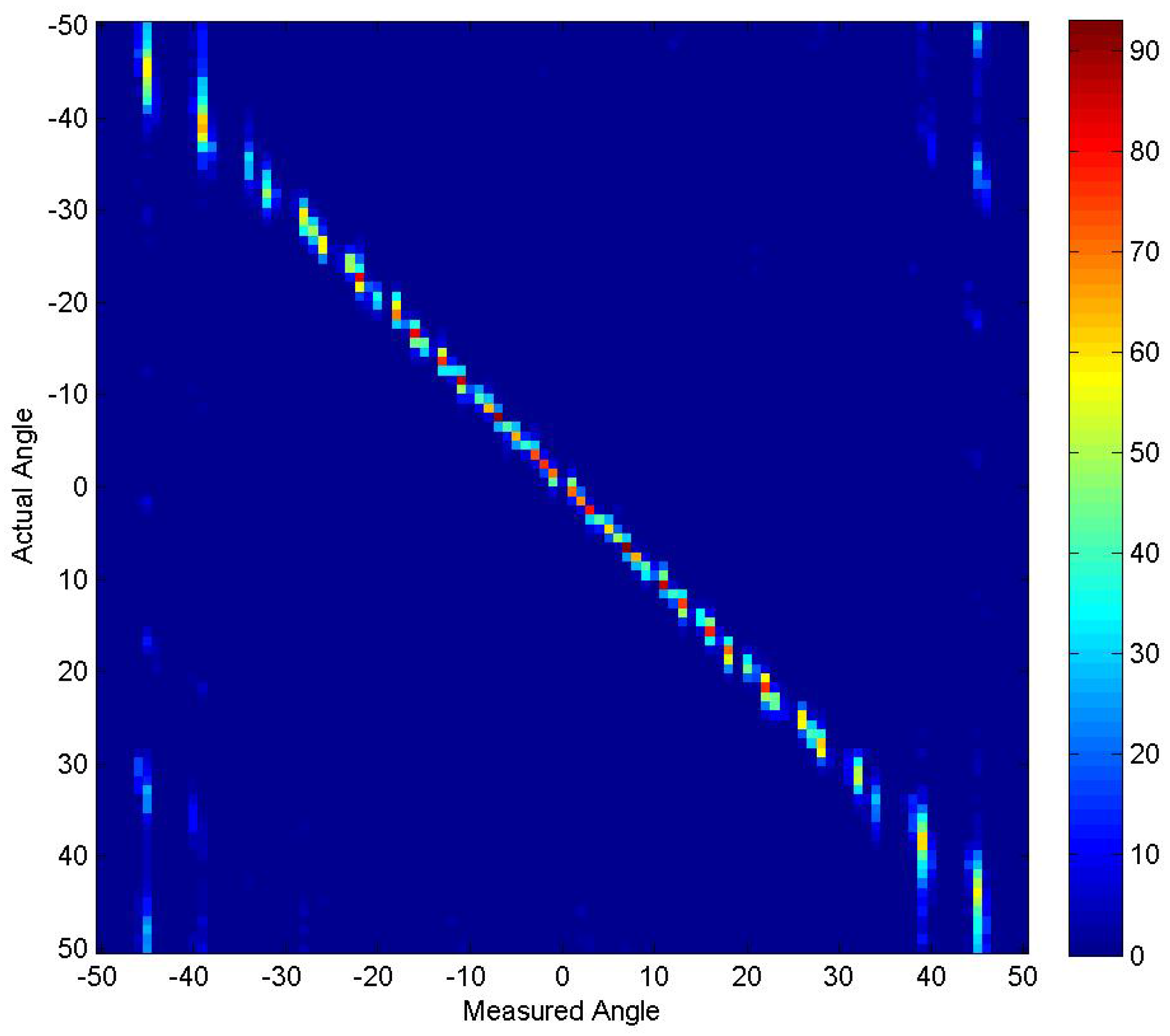
• In both cases, there were some beams that were placed very close together. This occurs a few times in the non-thresholded case where zero and 0.1 degrees are used along with 30.7 and 30.8 degrees. In all likelihood, these beams were not contributing and would have likely been optimized out had the GA continued to run longer.
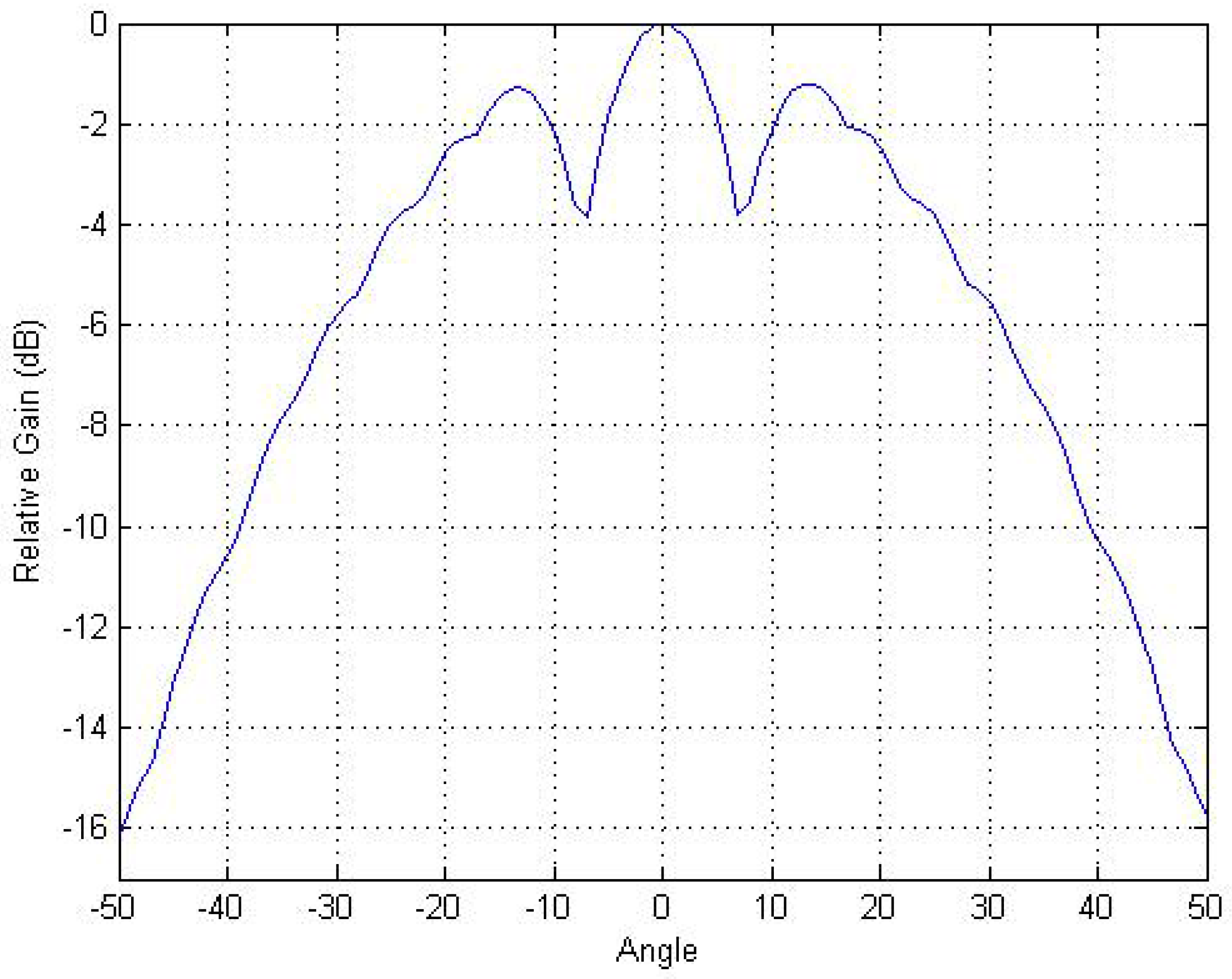
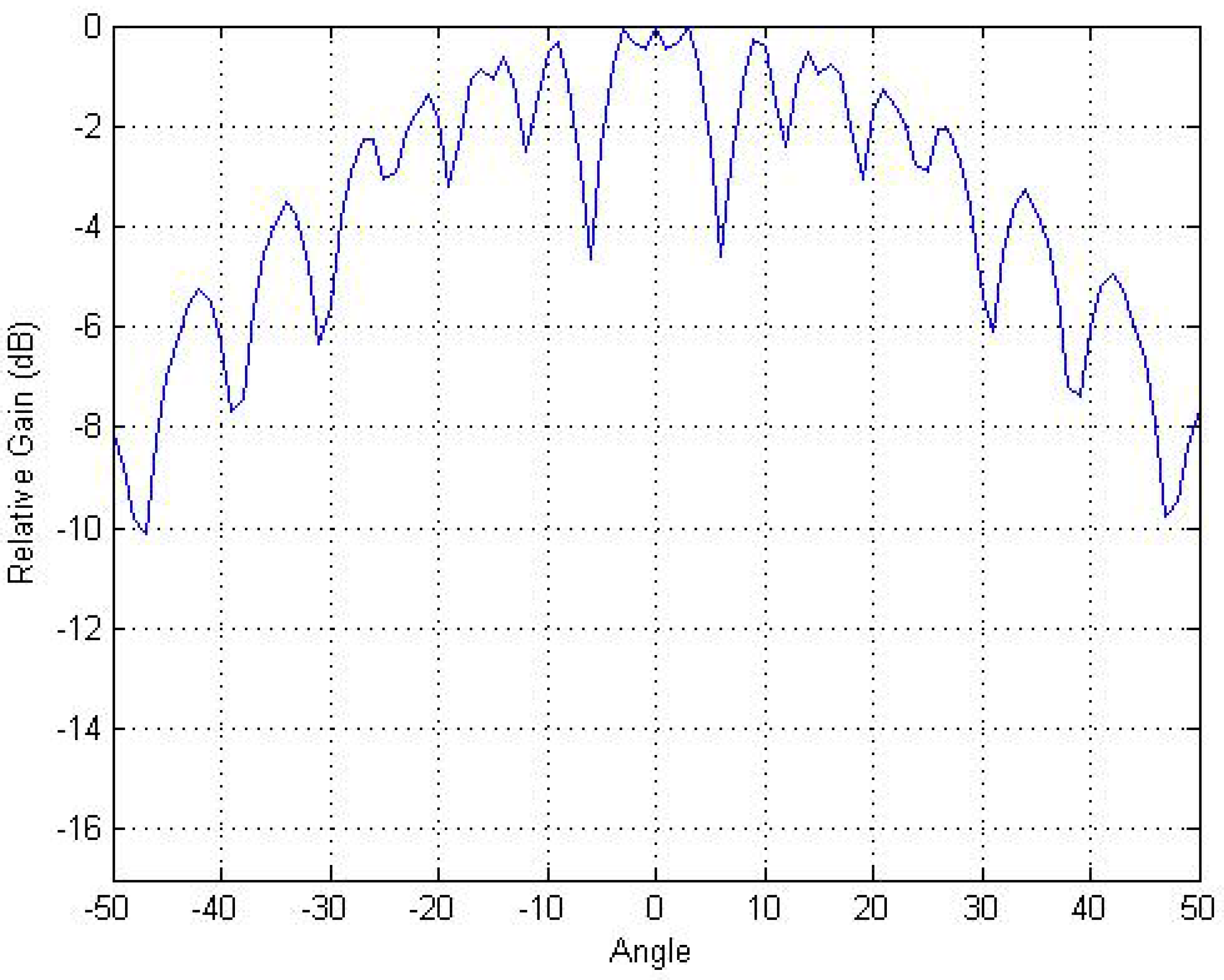
• The steered beams are more predominately steered away from the boresight. In both cases, the first effectively-steered beam occurs at 14 degrees. The GA may have been trying to direct more of the beams in those directions to minimize beam shape loss at those angles. The effect of this choice can be seen in Figure 4 where there are 3-dB dips in the beam pattern around $\pm 7^{\circ }$.

The minimum fitness score from each generation is shown in Figure 5a,b. The corresponding plots for the other experiments are very similar and do not provide any further value, so these are only shown for Experiment 1. The ambiguity plots are shown in Figure 6 and Figure 7.

4.2. Experiment 2

Experiment 2 was designed to fix the number of beams and weights while varying the number of elements and the element spacing. The purpose of this experiment was to validate our assumption that maximizing the number of receive elements and spacing them at half wavelengths would maximize performance. The parameter set chosen by the GA and the final fitness score for this experiment are shown in

Table 8. Experiment 2 results.

Description	Value (No Threshold)	Value (13-dB Threshold)
Number of transmit elements	1	1
Number of receive elements	8	8
RX array element spacings (in lambda)	0.95, 0.5, 0.99, 0.97, 0.82, 0.9, 0.99	0.81, 0.95, 0.98, 0.51, 0.81, 0.5, 0.7
Number of steered beams	21	21
Steering angles in degrees	0, ±(5, 10, 15, 20, 25, 30, 35, 40, 45, 50)	0, ±(5, 10, 15, 20, 25, 30, 35, 40, 45, 50)
Receive element weights	1	1
Fitness score (${\mathit{MSE}}^{\mathbf{\circ }}$)	2.21	2.16

. Bold values in the table show numbers optimized by the GA.

There were several surprises from these results. The first surprise was that the GA decided to use a single transmit element instead of two. While this does increase the beam width, it does so at the cost of a loss in performance at and near boresight due do the drop in transmit antenna gain. We believe this behavior may be an artifact of how the simulator works. The simulator models a target with a specified boresight SNR. That target is then simulated across the field of view, effectively at a constant range. What this means is that for a target to be detectable near the edge of the field of view, it must have a relatively strong SNR at the boresight.

Going back to the decision of the GA to use a single transmit element, we believe this was done because the SNR of the target was sufficiently strong enough near the center of the field of view that the penalty imposed by dropping to a single transmit element was less than what was gained by widening the beam pattern. Looking back at the results of the baseline test and the results from Experiment 1, it is obvious that the main contributing factor to the high mean squared error is the radar’s performance near the edge of the field of view. The GA decided that widening the beam pattern was the best way to reduce the ambiguity in those areas.

Another interesting observation from this experiment was the element spacings that were chosen by the GA. The assumption going into this analysis was that spacings much larger than half the wavelength would introduce grating lobes that would create ambiguities in the localization algorithm resulting in high $MS{E}^{\circ }$ numbers. This was not the case. In most cases, all of the element spacings are close to the maximum allowed, except for one or two, which are always near half the wavelength. This behavior is not yet well understood and is discussed further in the Future Work section of the document. The ambiguity plots are shown in Figure 8 and Figure 9.

4.3. Experiment 3

This experiment used the same number of elements and the same element spacing that was used by the baseline test. The GA was used to vary the number of beams, steering angles and element weights. Our expectation with this experiment was that the GA would chose similar steering angles from what was chosen in Experiment 1. We also assumed that the element weights would all be close to one to maximize the SNR. The parameter set chosen by the GA and the final fitness score for this experiment are shown in

Table 9. Experiment 3 results.

Description	Value (No Threshold)	Value (13-dB Threshold)
Number of transmit elements	2	2
Number of receive elements	8	8
Array element spacings (in lambda)	0.5	0.5
Number of steered beams	21	21
Steering angles in degrees	0, ±(0.9, 13.3, 19.5, 24.1, 27.3, 28.9, 38.9, 42.3, 48.1, 59.2)	0, ±(1.1, 6.8, 11.5, 15, 16.9, 20.4, 23, 25, 25.4, 38)
Receive element weights	0.95, 0.32, 0.52, 0.28, 0, 0.32, 0.65, 0.89	0.19, 0.13, 0.36, 0.48, 0.98, 0.66, 0.2, 0.27
Fitness score (${\mathit{MSE}}^{\mathbf{\circ }}$)	4.06	2.85

. Bold values in the table show numbers optimized by the GA.

The results of the chosen steering angles for the no threshold case were not that surprising. The values were very similar to the kinds of values that were obtained in Experiment 1 where the beams were directed more towards the edge of the field of view. In the thresholded case however, the beams were directed closer to the boresight. This is likely due to the low number of detections near the edge of the field of view, which may have encouraged the GA to direct less energy in that direction. The current implementation of the fitness score does not penalize configurations that have a reduced field of view. This can encourage the GA to come up with solutions that may not be ideal in a real design.

There selected receive element weights were also unexpected. The GA chose a weight of zero for one of the elements in the no threshold case. What makes this interesting is that the element spacings were fixed to half wavelength spacing in this experiment. Therefore, by setting one particular element’s weight to zero, the GA essentially removed it from the design. This allowed it to achieve a larger than half lambda spacing at the expense of sacrificing a receive element that reduces the target SNR. The GA effectively found a way around one of the restrictions that was placed on it. The ambiguity plots are shown in Figure 10 and Figure 11.

4.4. Experiment 4

This experiment essentially gives the GA free reign over the entire suite of radar parameters. It allows the GA to optimize the number of elements, spacing, weights and the number of beams. The point of this experiment was to determine how well the GA could cope with a very large solution space and to see what kind of solutions it would come up with under these conditions. The parameter set chosen by the GA and the final fitness score for this experiment are shown in

Table 10. Experiment 4 results.

Description	Value (No Threshold)	Value (13-dB Threshold)
Number of transmit elements	1	1
Number of receive elements	8	8
Array element spacings (in lambda)	0.97, 0.6, 0.84, 0.88, 0.77, 0.52, 0.5	0.93, 0.77, 0.54, 0.8, 0.51, 0.84, 0.83
Number of steered beams	21	21
Steering angles in degrees	0, ±(2.8, 9.4, 14.1, 16.4, 21.2, 26.7, 34.2, 42.4, 52, 59.8)	0, ±(1.5, 7.1, 9.9, 20.5, 26.5, 31.2, 37.8, 43.4, 51.3, 56.8)
Receive element weights	0.92, 0.01, 0.58, 0.75, 0.48, 0.79, 0.01, 0.68	0.4, 0.3, 0.29, 0.49, 0.64, 0.4, 0.99, 0.78
Fitness score (${\mathit{MSE}}^{\mathbf{\circ }}$)	1.76	1.75

. Bold values in the table show numbers optimized by the GA.

This particular experiment yielded some of the lowest $MS{E}^{\circ }$ results from all of the testing that was performed. Several of the other experiments resulted in steering angles that were concentrated towards the edge of the field of view. In this experiment where the element spacing and weight were also being varied, the GA decided that a more even spacing was the best approach. This experiment also repeated the behavior of selecting extremely low weights for some elements to achieve a greater than one wavelength spacing. The ambiguity plots are shown in Figure 12 and Figure 13.

4.5. Experiment 5

Experiment 5 was designed to take the learning from Experiments 1–4 and restrict the parameter set for the GA to search over. The idea was that this would reduce the search space, thus allowing the GA to find a better solution than what was found in Experiment 4. For this experiment, the number of transmit and receive elements and the number of beams was fixed. The steering angles, element spacings and element weights were varied by the GA. The parameter sets chosen by the GA and the final fitness score for this experiment are shown in

Table 11. Experiment 5 results.

Description	Value (No Threshold)	Value (13-dB Threshold)
Number of transmit elements	1	1
Number of receive elements	8	8
Array element spacings (in lambda)	0.99, 1.0, 0.79, 0.89, 0.57, 0.66, 0.9	0.6, 0.6, 0.88, 0.86, 0.7, 0.85, 0.78
Number of steered beams	21	21
Steering angles in degrees	0, ±(11.8 13.8 17.5 27.7, 31.5, 36.8, 42, 46.1, 49, 57.8)	0, ±(4.2, 10.1, 15.5, 18.6, 21.3, 27.6, 33.4, 38.7, 45, 52.4)
Receive element weights	0.82, 0.61, 0.82, 0.06, 0.21, 0.68, 0.44, 0.57	0.31, 0.13, 0.16, 0.38, 0.95, 0.84, 0.31, 0.41
Fitness score (${\mathit{MSE}}^{\mathbf{\circ }}$)	1.74	1.84

. Bold values in the table show numbers optimized by the GA.

While the solutions that were selected in Experiment 5 were very different from those selected in Experiment 4, the end result was similar. The most likely explanation is that even though the search space was reduced by several orders of magnitude, it was not reduced enough to make any meaningful difference. Figure 14 shows the beam forming envelope off all of the beams for Experiment 5 (no threshold). The ambiguity plots are shown in Figure 15 and Figure 16.

5. Conclusions

The primary goal behind this work was to show that a GA could be used to optimize several key radar design parameters related to beamforming and angle of arrival performance. In our experiments, we were able to show that the GA was able to generate a solution that more than halved the mean squared error versus a human-made design. With a more sophisticated objective function that takes into account the cost of some of the design parameters, this approach could be used to design an actual radar. A summary of the results is shown in

Table 12. Results’ summary.

Experiment	Parameters Varied	MSE (No Threshold)	MSE (13-dB Threshold)
Baseline	All Fixed	6.57	4.77
Exp. 1	Number/Angle of Steered Beams	5.24	3.88
Exp. 2	Number of TX/RX Elements and Their Spacings	2.21	2.16
Exp. 3	Number/Angle of Steered Beams and Weights	4.06	2.85
Exp. 4	All	1.76	1.75
Exp. 5	Element Spacing/Weights and Steering Angles	1.74	1.84

. Bold values in the table show the best optimziation results.

The GA highlighted its ability to find good solutions in a very large search space in a reasonable amount of time. It was also able to work around constraints, such as fixed element spacings, to achieve better results. It also came up with several unintuitive solutions that worked well.

The beamforming and localization simulator that served as the objective function for the GA also worked well for this application. Extensive use of vector operations inside this MATLAB program enabled it to execute quickly enough for our needs.

6. Future Work

Several areas of future work were identified as part of this study. These are listed below.

• The localization simulator uses a specified target SNR at the boresight and calculates what that target’s SNR would be at different angles to the radar. This effectively allows the simulator to evaluate the performance of the system at some given range. The problem with this approach is that it does not allow the user to evaluate system performance at the edge of detection range across the entire field of view. A target with a very low SNR near the edge of the field of view will have a much stronger SNR at the boresight. This can lead the GA to come up with optimization solutions that work well at a particular range, but it may perform very poorly at further ranges. The next step with this evaluation is to modify the simulator to model a target with a given SNR (likely the minimum detectable SNR) across the entire field of view. This would allow the GA to optimize a solution that works the best for the worst case.
• Expanding on the previous item, this approach could be used to optimize parameters that can be configured on the fly for different target SNRs.
• The simulations that were performed only covered a ±50 degree field of view. It is very likely that the solutions the GA came up with have ambiguities outside of that region. Follow up work should be done to analyze these radar parameters with a wider coverage area. It would also be good to see what kind of solutions the GA comes up with when presented with a wider field of view.
• The localization simulator currently only supports localization in the azimuth direction. The program could be expanded to simulate and evaluate performance across both azimuth and elevation. The drawback of doing this is an explosion in computational complexity, which would require the use of far more powerful hardware than what was used for this evaluation.
• This program simulates a target in free space. In an actual radar design, clutter sources at the same range as the target can negatively effect localization performance. Digitally-formed beams with wide beam widths or strong sidelobes are more susceptible to these negative effects. The localization simulator could be updated to model this behavior, which would allow the GA to come up with a solution that works better in cluttered environments.
• The fitness score returned by the objective function in this algorithm is based solely on mean squared error. In an actual radar, there are other design considerations that should be accounted for. For example:

  • The number of transmit and receive elements used in a radar design have a significant impact on the cost of the system, the computational resources required to support the signal processing and the power used by the radar. In addition to this, the number of patch elements along with how far apart they are spaced effects the size of the radar, as well, which may be critical to the design of the system.
  • The number of beams to digitally form also has a computational cost associated with them, which is not captured by the algorithm. Supporting a large number of digitally-steered beams may not be feasible for some applications.
  • The objective function does not take the detectable field of view into consideration when generating a fitness score. This algorithm could be updated to include that design parameter in its fitness score. Solutions that do not meet the desired field of view would be penalized.
  Given that these costs are not accounted for, the GA does not consider those impacts when optimizing the radar design parameters.
• Some radars use beam spoiling, a process where the transmit beam is widened using digital beamforming techniques. We would like to add beam spoiling capability rather than restrict the number of transmit elements, since this will lower the overall transmit power.
• The reasoning for why the GA frequently chose large element spacings and why it seemed to improve performance is still not well understood. Performing a more detailed analysis of one of these configurations may shed more light on this phenomenon.

References

1. San Antonio, G.; Fuhrmann, D.R. Beampattern synthesis for wideband MIMO radar systems. In Proceedings of the 2005 1st IEEE International Workshop on Computational Advances in Multi-Sensor Adaptive Processing, Puerto Vallarta, Mexico, 13–15 December 2005; pp. 105–108.
2. Bonyadi, M.R.; Michalewicz, Z. Particle swarm optimization for single objective continuous space problems: A review. Evol. Comput. 2016, 25, 1–54. [Google Scholar] [CrossRef] [PubMed]
3. Wilke, D.N.; Kok, S.; Groenwold, A.A. Comparison of linear and classical velocity update rules in particle swarm optimization: Notes on diversity. Int. J. Numer. Methods Eng. 2007, 70, 962–984. [Google Scholar] [CrossRef]
4. Poli, R.; Kennedy, J.; Blackwell, T. Particle swarm optimization. Swarm Intell. 2007, 1, 33–57. [Google Scholar] [CrossRef]
5. Poli, R. Analysis of the publications on the applications of particle swarm optimisation. J. Artif. Evol. Appl. 2008, 2008, 685175. [Google Scholar] [CrossRef]
6. Mehrabian, A.R.; Lucas, C. A novel numerical optimization algorithm inspired from weed colonization. Ecol. Inform. 2006, 1, 355–366. [Google Scholar] [CrossRef]
7. Mitchell, M. An Introduction to Genetic Algorithms; MIT Press: Cambridge, MA, USA, 1998. [Google Scholar]
8. Golberg, D.E. Genetic algorithms in search, optimization, and machine learning. Addion Wesley 1989, 1989, 102. [Google Scholar]
9. Mavromatidis, L.E. A review on hybrid optimization algorithms to coalesce computational morphogenesis with interactive energy consumption forecasting. Energy Build. 2015, 106, 192–202. [Google Scholar] [CrossRef]
10. Marin, P.; Marsault, X.; Mavromatidis, L.E.; Saleri, R.; Torres, F. Ec-Co-Gen: An evolutionary simulation assisted design tool for energy rating of buildings in early design stage to optimize the building form. In Proceedings of the BS2013, Chambery, France, 26–28 August 2013.
11. Jones, G.; Willett, P.; Glen, R.C. Molecular recognition of receptor sites using a genetic algorithm with a description of desolvation. J. Mol. Biol. 1995, 245, 43–53. [Google Scholar] [CrossRef]
12. Deaven, D.M.; Ho, K.M. Molecular geometry optimization with a genetic algorithm. Phys. Rev. Lett. 1995, 75, 288. [Google Scholar] [CrossRef] [PubMed]
13. Zwickl, D.J. Genetic Algorithm Approaches for the Phylogenetic Analysis of Large Biological Sequence Datasets under the Maximum Likelihood Criterion. Ph.D. Thesis, The University of Texas at Austin, Austin, TX, USA, 2006. [Google Scholar]
14. Hassan, R.; Cohanim, B.; De Weck, O.; Venter, G. A comparison of particle swarm optimization and the genetic algorithm. In Proceedings of the 46th AIAA/ASME/ASCE/AHS/ASC Structures, Structural Dynamics and Materials Conference, Austin, TX, USA, 18–21 April 2005; p. 1897.
15. Zaharis, Z.D.; Gotsis, K.A.; Sahalos, J.N. Adaptive beamforming with low side lobe level using neural networks trained by mutated boolean PSO. Prog. Electromagn. Res. 2012, 127, 139–154. [Google Scholar] [CrossRef]
16. Zaharis, Z.D.; Yioultsis, T.V. A novel adaptive beamforming technique applied on linear antenna arrays using adaptive mutated boolean PSO. Prog. Electromagn. Res. 2011, 117, 165–179. [Google Scholar] [CrossRef]
17. Zaharis, Z.D.; Skeberis, C.; Xenos, T.D. Improved antenna array adaptive beamforming with low side lobe level using a novel adaptive invasive weed optimization method. Prog. Electromagn. Res. 2012, 124, 137–150. [Google Scholar] [CrossRef]
18. Roy, G.G.; Das, S.; Chakraborty, P.; Suganthan, P.N. Design of non-uniform circular antenna arrays using a modified invasive weed optimization algorithm. IEEE Trans. Antennas Propag. 2011, 59, 110–118. [Google Scholar] [CrossRef]
19. Basak, A.; Pal, S.; Das, S.; Abraham, A. Circular antenna array synthesis with a differential invasive weed optimization algorithm. In Proceedings of the 2010 10th International Conference on Hybrid Intelligent Systems (HIS), Atlanta, GA, USA, 23–25 August 2010; pp. 153–158.
20. Basak, A.; Pal, S.; Das, S.; Abraham, A.; Snasel, V. A modified invasive weed optimization algorithm for time-modulated linear antenna array synthesis. In Proceedings of the 2010 IEEE Congress on Evolutionary Computation (CEC), Barcelona, Spain, 18–23 July 2010; pp. 1–8.
21. Bhattacharya, R.; Bhattacharyya, T.K.; Saha, S. Sidelobe level reduction of aperiodic planar array using an improved invasive weed optimization algorithm. In Proceedings of the 2011 IEEE Applied Electromagnetics Conference (AEMC), Kolkata, India, 18–22 December 2011; pp. 1–4.
22. Pappula, L.; Ghosh, D. Large array synthesis using invasive weed optimization. In Proceedings of the 2013 International Conference on Microwave and Photonics (ICMAP), Dhanbad, India, 13–15 December 2013; pp. 1–6.
23. Mallahzadeh, A.R.R.; Oraizi, H.; Davoodi-Rad, Z. Application of the invasive weed optimization technique for antenna configurations. Prog. Electromagn. Res. 2008, 79, 137–150. [Google Scholar] [CrossRef]
24. Capraro, C.T.; Bradaric, I.; Capraro, G.T.; Lue, T.K. Using genetic algorithms for radar waveform selection. In Proceedings of the 2008 IEEE Radar Conference, Rome, Italy, 26–30 May 2008; pp. 1–6.
25. Chan, K.C.C.; Lee, V.; Leung, H. Generating fuzzy rules for target tracking using a steady-state genetic algorithm. IEEE Trans. Evol. Comput. 1997, 1, 189–200. [Google Scholar] [CrossRef]
26. Lin, Y.; Bhanu, B. Evolutionary feature synthesis for object recognition. IEEE Trans. Syst. Man Cybern. Part C Appl. Rev. 2005, 35, 156–171. [Google Scholar] [CrossRef]
27. Kurdzo, J.M.; Palmer, R.D. On the use of genetic algorithms for optimization of a multi-band, Multi-Mission radar network. In Proceedings of the 2011 IEEE RadarCon (RADAR), Kansas City, MO, USA, 23–27 May 2011; pp. 231–236.
28. Orfila, A.; Molcard, A.; Sayol, J.M.; Marmain, J.; Bellomo, L.; Quentin, C.; Barbin, Y. Empirical Forecasting of HF-Radar Velocity Using Genetic Algorithms. IEEE Trans. Geosci. Remote Sens. 2015, 53, 2875–2886. [Google Scholar] [CrossRef]
29. Kristoffersen, S.; Moen, H.J.F. Denial jamming technique development against pulse-doppler radars using genetic algorithms. In Proceedings of the 2008 International Conference on Radar, Rome, Italy, 26–30 May 2008; pp. 253–258.
30. Richards, M.A. Fundamentals of Radar Signal Processing; Tata McGraw-Hill Education: New York, NY, USA, 2005. [Google Scholar]
31. Li, J.; Stoica, P. Robust Adaptive Beamforming; John Wiley & Sons: Hoboken, NJ, USA, 2005; Volume 88. [Google Scholar]
32. Harter, M.; Ziroff, A.; Zwick, T. Three-dimensional radar imaging by digital beamforming. In Proceedings of the 2011 European Radar Conference (EuRAD), Manchester, UK, 12–14 October 2011; pp. 17–20.
33. Chang, P.R.; Yang, W.H.; Chan, K.K. A Neural Network Approach to MVDR Beamforming Problem. IEEE Trans. Antennas Propag. 1986, 34, 8190–8192. [Google Scholar]
34. Southall, H.; Simmers, J.A.; O’Donnell, T.H. Direction Finding in Phased Arrays with a Neural Network Beamformer. IEEE Trans. Antennas Propag. 1995, 43, 1369–1374. [Google Scholar] [CrossRef]
35. Jha, S.; Durrani, T. Direction of arrival estimation using artificial neural networks. IEEE Trans. Syst. Man Cybern. 1991, 21, 1192–1201. [Google Scholar] [CrossRef]
36. Shieh, C.S.; Lin, C.T. Direction of Arrival Estimation Based on Phase Differences Using Neural Fuzzy Network. IEEE Trans. Antennas Propag. 2000, 48, 1115–1124. [Google Scholar] [CrossRef]
37. Yang, W.H.; Chan, K.K.; Chang, P.R. Complex-valued neural network for direction of arrival estimation—Electronics Letters. Electron. Lett. 1994, 30, 2–3. [Google Scholar] [CrossRef]
38. Agatonovic, M.; Stankovic, Z.; Milovanovic, I.; Doncov, N.; Sit, L.; Zwick, T.; Milovanovic, B. Efficient neural network approach for 2D DOA estimation based on antenna array measurements. Prog. Electromagn. Res. 2013, 137, 741–758. [Google Scholar] [CrossRef]
39. Lo, T.; Leung, H.; Litva, J. Radial Basis Function Neural Network for Direction-of-Arrivals Estimation. IEEE Signal Process. Lett. 1994, 1, 45–47. [Google Scholar] [CrossRef]
40. Zaman, F.; Qureshi, I.M.; Naveed, A.; Khan, J.A.; Asif Zahoor, R.M. Amplitude and directional of arrival estimation: Comparison between different techniques. Prog. Electromagn. Res. B 2012, 39, 319–335. [Google Scholar] [CrossRef]
41. Page, R.M. Simultaneous Lobe Comparison, Pulse Echo Locator System. U.S. Patent 2,929,056, 15 March 1960. [Google Scholar]
42. Capon, J. High-resolution frequency-wavenumber spectrum analysis. Proc. IEEE 1969, 57, 1408–1418. [Google Scholar] [CrossRef]
43. Viberg, M.; Ottersten, B.; Nehorai, A. Performance analysis of direction finding with large arrays and finite data. IEEE Trans. Signal Process. 1995, 43, 469–477. [Google Scholar] [CrossRef]
44. Schmidt, R. Multiple emitter location and signal parameter estimation. IEEE Trans. Antennas Propag. 1986, 34, 276–280. [Google Scholar] [CrossRef]
45. Ren, Q.; Willis, A. Fast root MUSIC algorithm. Electron. Lett. 1997, 33, 450–451. [Google Scholar] [CrossRef]
46. Roy, R.; Kailath, T. ESPRIT-estimation of signal parameters via rotational invariance techniques. IEEE Trans. Acoust. Speech Signal Process. 1989, 37, 984–995. [Google Scholar] [CrossRef]
47. Page, R.M. Accurate Angle Tracking by Radar (Naval Research Laboratory Formal Report RA-3A-222A); Technical Report; Naval Research Laboratory: Washington, DC, USA, 1944. [Google Scholar]
Figure 1. Sample AOA ambiguity plot.
Electronics 06 00024 g001
Figure 2. Ambiguity plot for baseline radar configuration (no detection threshold).
Electronics 06 00024 g002
Figure 3. Ambiguity plot for baseline radar configuration (13-dB detection threshold).
Electronics 06 00024 g003
Figure 4. Experiment 1 beamforming relative gain envelope to boresight (no threshold case).
Electronics 06 00024 g004
Figure 5. Experiment 1 minimum fitness score over each generation.
Electronics 06 00024 g005
Figure 6. Ambiguity plot for Experiment 1 (no threshold).
Electronics 06 00024 g006
Figure 7. Ambiguity plot for Experiment 1 (13-dB threshold).
Electronics 06 00024 g007
Figure 8. Ambiguity plot for Experiment 2 (no threshold).
Electronics 06 00024 g008
Figure 9. Ambiguity plot for Experiment 2 (13-dB threshold).
Electronics 06 00024 g009
Figure 10. Ambiguity plot for Experiment 3 (no threshold).
Electronics 06 00024 g010
Figure 11. Ambiguity plot for Experiment 3 (13-dB threshold).
Electronics 06 00024 g011
Figure 12. Ambiguity plot for Experiment 4 (no threshold).
Electronics 06 00024 g012
Figure 13. Ambiguity plot for Experiment 4 (13-dB threshold).
Electronics 06 00024 g013
Figure 14. Experiment 5 beamforming relative gain envelope to the boresight (no threshold case).
Electronics 06 00024 g014
Figure 15. Ambiguity plot for experiment 5 (no threshold).
Electronics 06 00024 g015
Figure 16. Ambiguity plot for Experiment 5 (13-dB threshold).
Electronics 06 00024 g016