An Energy Box in a Cloud-Based Architecture for Autonomous Demand Response of Prosumers and Prosumages

Abstract

The interest in the implementation of demand response programs for domestic customers within the framework of smart grids is increasing, both from the point of view of scientific research and from the point of view of real applications through pilot projects. A fundamental element of any demand response program is the introduction at customer level of a device, generally named energy box, able to allow interaction between customers and the aggregator. This paper proposes two laboratory prototypes of a low-cost energy box, suitable for cloud-based architectures for autonomous demand response of prosumers and prosumages. Details on how these two prototypes have been designed and built are provided in the paper. Both prototypes are tested in the laboratory along with a demonstration panel of a residential unit, equipped with a real home automation system. Laboratory tests demonstrate the feasibility of the proposed prototypes and their capability in executing the customers’ loads scheduling returned by the solution of the demand-response problem. A personal computer and Matlab software implement the operation of the aggregator, i.e., the intermediary of the energy-integrated community constituted by the customers themselves, who participate in the demand response program.

1. Introduction

Many attractive definitions are currently used for demand response (DR); two of them are: “today’s killer app for smart grid” and “the key for engaging consumers in the smart grid”. A conventional definition states that DR is a program of actions, aimed at changes in habits of end-use customers in consuming energy [1]; these changes are mainly driven by price signals and discounted rates that discourage the use of electricity during peak hours and allow savings on bills [2]. The easiest way to induce a customer to change his habits in using electricity is to schedule its electric loads; the bigger the savings in the bill achieved through loads scheduling, the higher the participation of the customer in a DR program. A comprehensive view on technical methodologies and architecture, and socioeconomic and regulatory factors that could facilitate the uptake of DR is reported in [3]. In the path of change mentioned above, the customer does not act as an individual; on the contrary, the customer is a member of an integrated community, coordinated by an intermediary named aggregator or coalition coordinator [4,5,6,7].

In the framework of this integrated community, the aggregator and the customer communicate with each other very frequently; the energy box (EB) is the device, which interfaces the aggregator and the customer [3]. For instance, in [8], the EB is the instrument placing bids on the Portuguese tertiary market. The aggregator negotiates with the grid operator, placing a bid, which depends on bids previously returned by all EBs. Each EB can provide two different bids where the first pays for a change in the state of charge of batteries—optimally sized as in [9] and placed in the residential unit—whereas the second pays for a change in the temperature set point of air conditioning of the residential unit. In [10], the EB is a full energy home controller able to manage between five and ten loads; two Linux-based EBs mounted with a ZigBee controller for the Spanish and French trial are presented. Also in [11], the EB is a home controller for a cost-effective nonintrusive load monitor, which provides a mechanism to easily understand and control energy consumption as well as to securely permit reconfiguration and programming from anywhere. On the contrary, the EB presented in [12] is a sophisticated software for energy management systems, consisting of a suite of algorithms which support the sequential decision-making process under uncertainty in a stochastic dynamic programming network. Also, the EB presented in [13] is a software; more precisely, it is a unique decision-making algorithm which serves an automated DR program where the automated characteristic aims to reduce uncertainty and complexity of daily price fluctuation from the customer’s perspective. Lastly, the EB proposed in [14] provides the wind power measurements via a multilayer feed-forward back-propagation neural network.

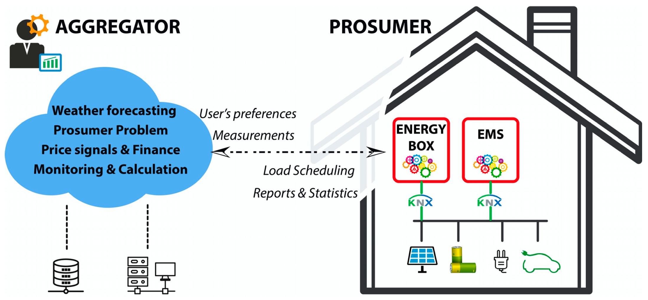
Given the aforementioned, the design of an EB is a hard task and full of challenges; a first and well-known challenge is to design the EB as a useful tool for communication between the consumer and the aggregator. A further challenge is to design an EB able to interact with the home energy management system (HEMS); this is because an HEMS, in general, does not necessarily share information and data (e.g., energy consumption measurements) with third parties, and it does not necessarily accept commands (e.g., turn on/off appliances) from third parties. In a residential unit, the HEMS is the device that monitors, controls and optimizes all peripherals, storage systems, distributed generators and smart meters, as illustrated in Figure 1. The HEMS asks the smart meters for energy consumptions so as to build a detailed and comprehensive status of the residential unit. Such a status is useful to precisely model and estimate energy consumption of the residential unit by using, as an example, a learning-based mechanism as in [15,16]. Therefore, the interoperability between EB and HEMS is a crucial point for implementation of a DR program in a framework of integrated community. Interoperability must be ensured regarding the communication protocols, the data format and the physical media used for communication; interoperability must also be extended to smart meters and all peripherals [17] which operate in islanded mode or in absence of a HEMS. When the same vendor produces the EB, the HEMS, the smart meters, the smart plugs and peripherals, the full interoperability is implicitly achieved; on the contrary, the management of devices produced by different vendors is much more difficult. A last challenge is to design the EB as a cost-effective tool if this technology is intended for a large number of customers, including less affluent people.

This paper proposes a new EB as a viable solution to the challenge of the communication between consumer and aggregator, and to the challenge of the interaction between an EB and HEMS. The paper also illustrates two prototypes of the proposed EB to have a clear overview of management and material requirements, as well as of cost-effectiveness; both prototypes are tested in the lab using a real home automation system.

Concerning the communication between the consumer and the aggregator, the proposed EB communicates with the aggregator’s IT platform and requires access to an application, service or system [18]. Communication is over the Internet and is based on the traditional client–server paradigm; HyperText Transfer Protocol over Secure Socket Layer (HTTPS) is the communication protocol used for secure communication. As illustrated in Figure 1, the proposed EB connects to the aggregator, uploads the user’s preferences and requires access to the application called prosumer problem; the application responds by providing the optimal loads scheduling. Furthermore, as in Figure 1, the EB uploads power/voltage/current measurements and it requires access to the service called monitoring and calculation; the service responds by providing reports and statistics.

Concerning the interaction with a HEMS, the proposed EB overcomes the problem of interaction because it directly communicates with all peripherals of the home automation system, bypassing the HEMS as in Figure 1. In particular, the proposed EB generates the control frames to turn on/off a load or to acquire a measurement from a meter; then, the EB sends these frames to loads and meters via the physical media for the communication of the home automation system, i.e., the typical shielded-twisted pair cable. Since the proposed EB bypasses the HEMS, two significant benefits are achieved. The first advantage is to overcome the obstacles placed by the HEMSs currently available on the market regarding the connection to devices supplied by third parties. Indeed, while HEMS are equipped with USB, RJ45 or RS482 ports for a peer-to-peer connection to EBs, a time-consuming configuration of both of these devices is usually necessary, in absence of any guarantee of obtaining a proper interaction and interoperability. The second advantage is to provide the DR program with the diagnostic, monitoring and control functions. While very important, these functions are not performed by the HEMSs currently available on the market or they are performed with insufficient quality. As a remedy, the proposed EB can be successfully adopted because it is unchained to HEMS and the valuable functions implemented by the EB are not stifled by the limits of the HEMS itself. In particular, the proposed EB uses easy programming languages to enable the expert customer to autonomously run a DR program and implement new functions and procedures that best meet its own needs.

Concerning the management and material requirements also in terms of cost-effectiveness, the two prototypes of the proposed EB were designed and tested in the laboratory; tests were carried out in conjunction with a demonstration panel of a residential unit, equipped with a real home automation system by Schneider Electric. The first prototype has a limited calculation capability and a low-cost (low-EB), the second prototype has a higher cost but also a higher capacity for solving calculation problems (high-EB). The low-EB prototype communicates with the aggregator over the internet to exchange data and submit service requests; in particular, it asks and receives from the aggregator the optimum scheduling of the consumer’s loads. The low-EB prototype applies scheduling without the help of HEMS by sending the on/off commands to the peripherals of the automation system. The high-EB prototype performs the same functions as the low-EB prototype, and in addition, it is capable of calculating optimum scheduling of consumer loads.

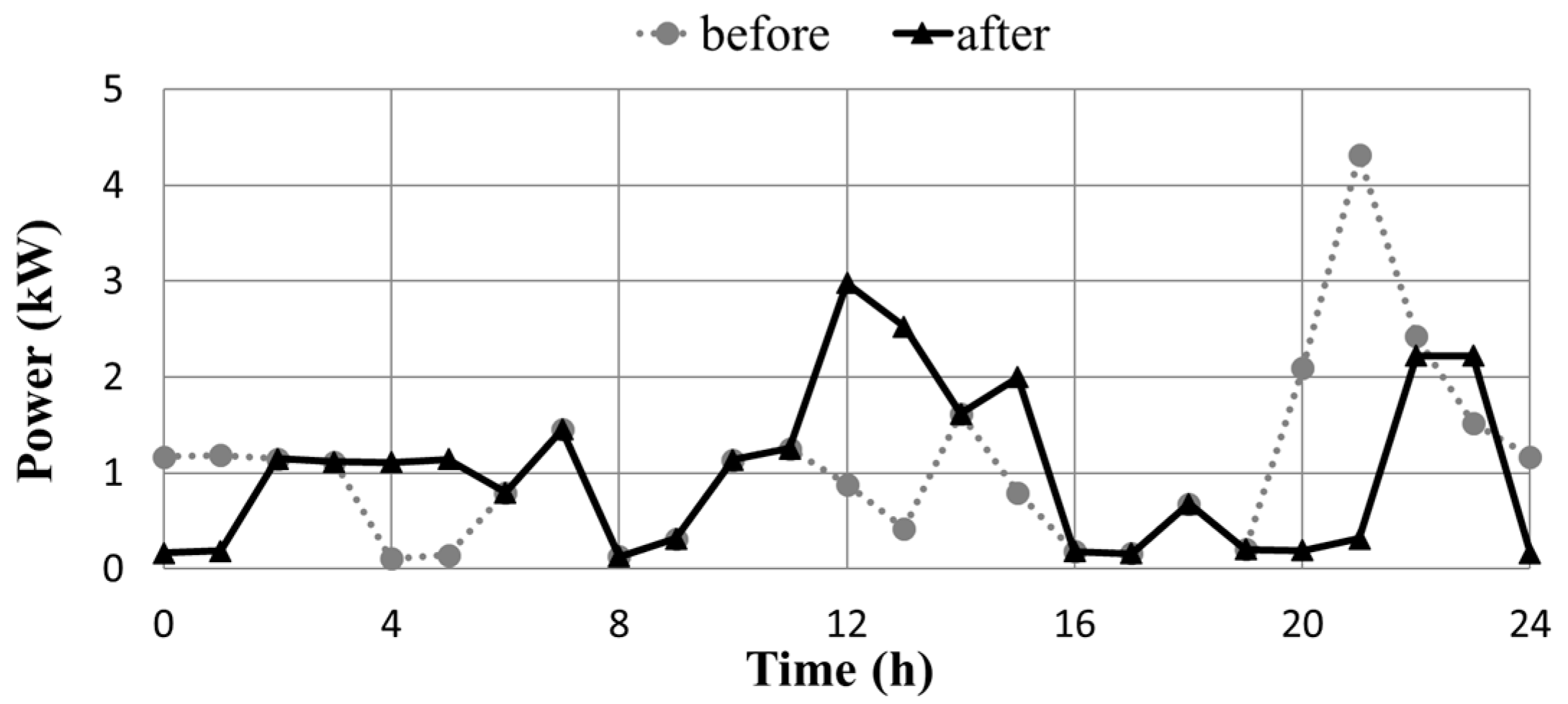
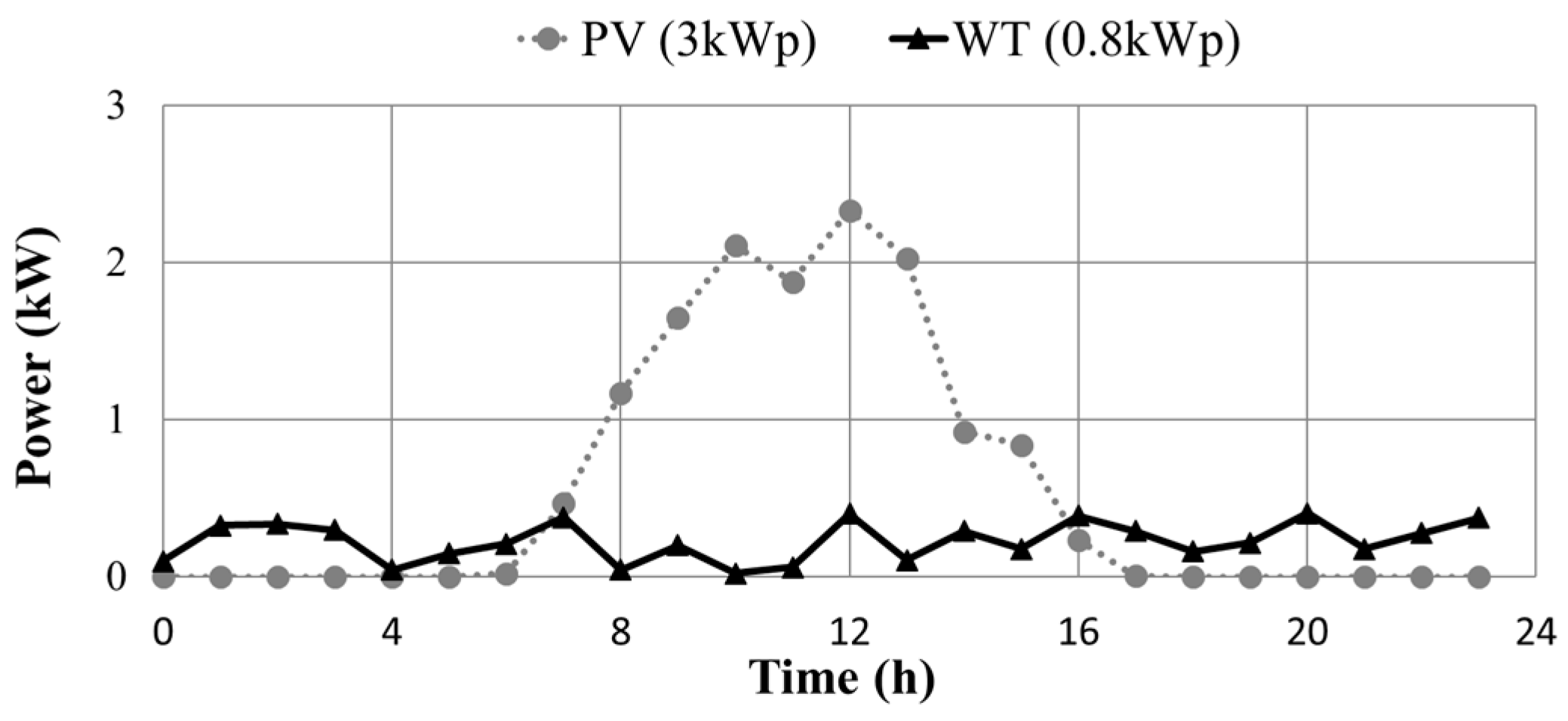
This paper is organized as follows. Section 2 illustrates a home energy management system problem, namely “prosumer problem”; it optimizes the loads scheduling of a customer taking into account the distributed generators, the energy storage systems, the daily fluctuation in electricity prices and loads demand. Section 3 illustrates the case study of a grid-connected customer with a 3 kW PV plant and a 0.8 kW wind turbine; the customer is also equipped with a 3–6 kWh lithium-ion battery pack. Finally, Section 4 anticipates the conclusions and illustrates two laboratory prototypes of the proposed EB, namely low-EB and high-EB. The first of two prototypes uses an Arduino MEGA 2560, while the second prototype uses a Raspberry Pi3.

2. The Prosumer Problem

A home energy management system problem, henceforth referred to simply as «prosumer problem» and previously presented by the authors in [19], is illustrated in this section. The prosumer problem optimizes the operation of domestic appliances taking into account the daily fluctuation in electricity prices, an electric energy storage system of electrochemical cells, the power generated by distributed generators exploiting renewable energy sources (RESs) and by other programmable generators. Nonprogrammable distributed generators exploiting RESs are a photovoltaic (PV) plant and a micro wind turbine (WT); their 24 h production forecast is assumed to be available. 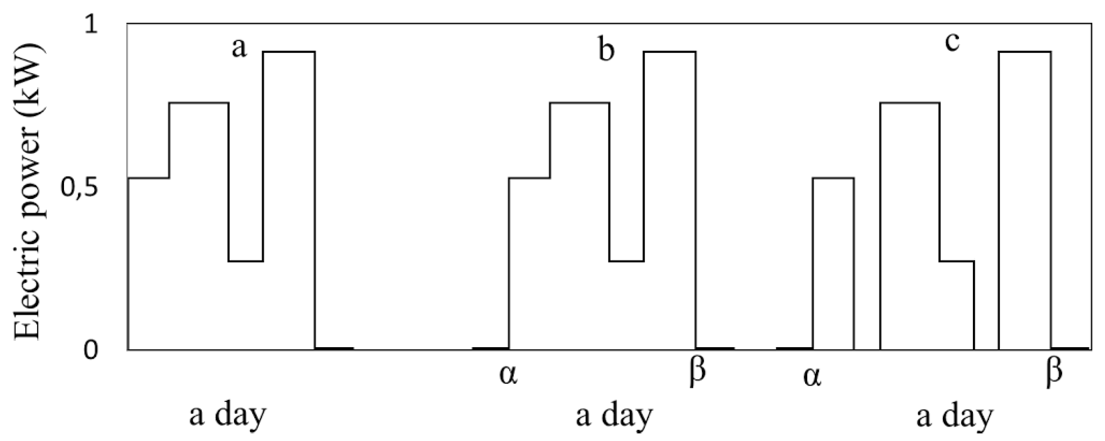In addition, a biomass boiler mounted with a free-piston Stirling engine and a linear electric generator realizes a micro combined heat and power generator (mCHP); this generator provides thermal power in the form of hot water and electric power [20]. It represents a programmable generator. The electric loads are divided into two groups, group A and group B. Schedulable loads and curtailable loads belong to group A; the lower case letter a is the index over this group. Non-controllable loads belong to group B; and the lower case letter b is the index over this group. As illustrated in Figure 2, the operating cycle of a non-controllable load is not subject to changes by third parties, therefore, this cycle is an input data for the prosumer problem. On the contrary, the operating cycle of a schedulable load can be entirely shifted in the time interval $\left[\alpha ,\beta \right]$, whereas the operating cycle of a curtailable load can be entirely or partially shifted in the time interval $\left[\alpha ,\beta \right]$. An optimization problem encapsulates the prosumer problem to return the load scheduling which minimizes the daily electricity cost:

$$min{\displaystyle \sum }_{h=1}^{24}\left\{c_{imp}{}^h·P_{imp}^h·∆t-c_{exp}{}^h·P_{exp}^h·∆t\right\},$$

(1)

subject to:

$$P_{imp}^h+P_{dis}^h+P_{WT}{}^h+P_{PV}{}^h+P_{mCHP}{}^h= P_{exp}^h+P_{cha}^h+{\displaystyle \sum }_{a=1}^A{y}_a^h·Ploa{d}_a+ {\displaystyle \sum }_{b=1}^{B}Ploa{d}_b^h,$$

(2)

$${\displaystyle \sum }_{h={\alpha }_a}^{{\beta }_a}{y}_a^h={\theta }_a,$$

(3)

$${\displaystyle \sum }_{h={\alpha }_a}^{{\beta }_a-{\theta }_a+1}{z}_a^h=1,$$

(4)

$$z_a^h=0 \forall h\in H-\left[{\alpha }_a,{\beta }_a-{\theta }_a+1\right],$$

(5)

$$y_a^h\ge z_a^h\forall h\in \left[{\alpha }_a,{\beta }_a\right],$$

(6)

$$y_a^{h+1}\ge z_a^h \forall h\in \left[{\alpha }_a,{\beta }_a\right],$$

(7)

$$y_a^{h+{\theta }_a-1}\ge z_a^h \forall h\in \left[{\alpha }_a,{\beta }_a\right],$$

(8)

$$0\le P_{imp}^h, P_{exp}^h\le P_{committed},$$

(9)

$$0\le P_{cha}^h\le m·P_{batt},$$

(10)

$$0\le P_{dis}^h\le P_{batt},$$

(11)

$$E_{STO}+{\displaystyle \sum }_{i=0}^h\left(\eta ·P_{cha}^i- P_{dis}^i\right)·∆t\ge \frac{SO{C}_{min}}{100}·C,$$

(12)

$$E_{STO}+{\displaystyle \sum }_{i=0}^h\left(\eta ·P_{cha}^i- P_{dis}^i\right)·∆t\le \frac{SO{C}_{max}}{100}·C,$$

(13)

m = recharge_current/discharge_current,

(14)

$$h\in \left[1\dots 24\right],$$

(15)

Equation (1) is the cost function, which calculates the daily net electricity cost as the difference between the import price $c_{imp}{}^h$ multiplied by the imported energy $P_{imp}^h·∆t$ and the export price $c_{exp}{}^h$ multiplied by the exported $P_{exp}^h·∆t$. Equation (2) is the power balance and imposes equality between the generated powers (exported to the grid, supplied by the batteries, produced by distributed generators) and the requested ones (imported from the grid, fed into the batteries, demanded by schedulable loads, demanded by non-controllable loads). $P_{PV}^h, P_{WT}^h and P_{mCHP}^h$ are the 24 h power generation forecast for the photovoltaic system, the micro wind turbine and the mCHP, respectively. The binary variable $y_a^h$ is 1 when the a-th schedulable load is turned ON at the h-th hour, it is zero and vice versa. Similarly, $P_{load}{}_b^h$ is the load demand of the b-th non-controllable schedulable load at the h-th hour. Equation (3) sets the duration of the operating cycle of each schedulable load, whereas Equations (4) and (5) define the start time of the operating cycle. Equations (6)–(8) ensure that the operating cycle is not divided into sub-cycles for non-curtailable loads. Equation (9) constrains the power flow between the grid and the prosumer at the point of delivery; power flow is upper bounded by the committed power. Equations (10) and (11) constrain the battery charge and discharge power flow. In particular, Equation (10) limits the recharge power $P_{cha}^h$ up to the batteries’ rated power multiplied by the coefficient m, defined in Equation (14) as the ratio between the recharge current and the discharge current. Equations (12) and (13) calculate the hourly state of charge (SOC) of the batteries, taking into account the state of charge at the beginning of the day, i.e., E_STO. Equation (14) returns the coefficient m as the ratio between the recharge and the discharge battery current; evidently, this coefficient takes into account battery technologies and the ability to charge the batteries with the current m times the discharge one. As an example, m is higher than 1 when Li-ion batteries are used, and m is lower than 1 when lead-acid batteries are used. The input data of the prosumer problem are:

-

the power forecast for generators, $P_{PV}^h$ and $P_{WT}^h$;

-

the hourly electricity prices, $Cim{p}^h$ and $Cex{p}^h$;

-

the load profiles of non-controllable loads, $Ploa{d}_b^h$;

-

the customer’s parameters, ${\alpha }_a$ and ${\beta }_a$.

3. The Case Study

The case study is a residential unit connected to the low voltage (230 V/50 Hz) distribution grid and equipped with distributed generators, an electric energy storage system and a home automation system.

3.1. Household Appliances and Electricity Demand

We considered common household appliances: internal and external lightings, a personal computer, a TV set, a refrigerator, an air-conditioning system, a washing machine, a tumble dryer, a dishwasher and an electric vehicle. In the case that the householder does not participate in any DR program, the electricity usage is the result of familiar habits. So, taking into account the statistical surveys reported in [21,22,23], the considered load demand profile is that reported in Figure 3 with a dotted line. The daily energy consumption is 24.97 kWh. The peak load is 4.31 kW at 21:00; the daily average load is 1.05 kW when the peak load value is considered, it decreases to 0.81 kW and vice versa.

3.2. Distributed Generators

Two distributed generators which exploit renewable energy sources contribute to satisfying the load demand; the first generator is a 3 kWp photovoltaic (PV) plant on the rooftop of a residential unit, the second one is a 0.8 kW wind turbine (WT) placed in the garden. The profile of the power generated by the PV plant and WT on 1 July 2015 are in Figure 4; real data measured in southern Italy were considered. The PV plant and the WT supply the local loads, then the batteries, and finally export into the grid.

3.3. Electric Energy Storage System

An electric energy storage system serves the residential unit so as to increase self-consumption. Among the storage technologies, batteries have been preferred due to their modularity and drive simplicity. In this paper lithium-ion batteries with a peak power of 3 kW and a capacity of 6 kWh are considered; the charge current is one time the discharge current. The round trip efficiency is 80%, the depth-of-discharge (SOC_min) is 30% and the depth-of-charge (SOC_max) is 98%. The self-discharge rate has been neglected. Since, as a hypothesis, the householder does not participate in a DR program, the PV plant and the WT recharge batteries when their generated power exceeds the load demand; the grid does not recharge or discharge the batteries. The state of charge of the batteries on 1 July 2015 is shown in Figure 5. The state of charge at midnight equals the SOC_min and batteries are temporally inoperative until the morning; from 8:00 to 12:00 the state of charge increases almost linearly from 30% up to 98%. From 12:00 to 20:00, the state of charge slightly changes and remains in the range of 75–98%; then it rapidly decreases to 30% in one hour.

3.4. Imported and Exported Electricity, Prices and Bill

Let us consider that an electricity retailer supplies power to the residential unit with a committed power equal to 6 kW. Given the load demand, the generation of distributed generators and the batteries, the power flow profile at the point of delivery is shown in Figure 6. Due to the sales contract signed between the retailer and the householder, both the import and the export prices change hourly as shown in Figure 7. The import price is calculated as the hourly wholesale market price plus a spread of 5% whereas the export price is calculated as the hourly zonal price minus a spread of 4% [24]. On 1 July 2015, the householder pays 0.52 € for energy consumption and power losses; on the other hand, he receives 0.15 € for exported energy. The daily net cost is 0.37 €.

3.5. Load Sharing between Distributed Generators and the Grid

The load demand is entirely satisfied by the distributed generators and the grid, without interruptions. With reference to Figure 8, the grid provides 40.28% of load demand while the distributed generators provide the remaining part. For the latter, 21.11% is directly provided by PV plant to loads, 20.06% is directly provided by the WT to loads, and the remaining 18.55% is indirectly provided through the batteries.

3.6. The Prosumer Problem Solution

As stated previously, for the householder who does not participate in any DR program, the electricity usage is the result of familiar habits: typically, family members leave the house in the morning and they return in the late afternoon. The electricity usage is the result of the load scheduling shown in Figure 9. Considering that the householder decides to participate in a DR program, household appliances are divided into the three load categories of Figure 2, namely non-controllable, shiftable and curtailable loads. Non-controllable loads include internal and external lightings, the personal computer, the TV set, the refrigerator and the air-conditioning system. Shiftable loads are: the washing machine (WM) and the tumble dryer (TD). Curtailable loads are: the dishwasher (DW) and the electric vehicle (EV). Being curtailable, the operating cycle of the DW and the EV can be divided in sub-cycles where each sub-cycle lasts 15 min or integer multiples of 15 min. It is worth noting that the tumble drier must start within 2 h of the end of the washing machine cycle. Shiftable loads parameters are collected in

Table 1. Shiftable appliances parameters.

Appliance	Power (kW)	Op. Cycle (min)	Curtailable	Time Interval αa–βa
Washing machine	2.1	120	no	21:00–19:00
Tumble dryer	1.2	60	no	21:00–19:00
Dish washer	1.9	120	yes	20:00–06:00
Electric vehicle	0.0 ÷ 3.0	0 ÷ 300	yes	19:00–07:00

where the last column reports the family members’ preference about the time interval, from α_a to β_a available to execute the entire operating cycle of each shiftable load. A fundamental hypothesis is that the accession of the householder to the DR program allows the aggregator to remotely manage the batteries placed in the residential unit. Therefore, the aggregator may require power exchanges between the batteries and the grid in order to achieve bill savings.

3.7. The Load Scheduling Returned by the the Prosumer Problem Solution and the Bill Saving

The loads scheduling returned by the prosumer problem solution is reported in Figure 10. With respect to the scheduling due to familiar habits in Figure 3, all these loads are time-shifted according to family members’ preferences, i.e., the parameters α_a and β_a. Familiar habits scheduled the recharge of the electric vehicle at midnight; now it is postponed by 2 h. The same delay is applied to the dishwasher. On the contrary, the washing machine and the tumble dryer are relevantly time-shifted; in particular, both these appliances are moved from the late evening to the early afternoon. On 1 July 2015, the householder now pays 0.58 € (it was 0.52 €) for the energy consumption and power losses; on the other hand, he receives 0.28 € (it was 0.15 €) for the exported electricity. The daily net cost now is 0.30 € (it was 0.37 €) therefore a 23.33% bill saving is achieved.

3.8. Power at the Point of Delivery after the Prosumer Problem Solution

The power flow profile at the point of delivery as returned by the application of the prosumer problem solution is illustrated in Figure 3 with a continuous line. Although the loads demand and the distributed generators generation remain unchanged, the daily energy exchanged at the point of delivery increases; this is because in a DR program the aggregator has the right to exchange power from the batteries to the grid and vice versa. By comparing the two lines of Figure 3, the electric energy drawn from the grid to the unit increases from 10.17 kWh to 13.6 kWh while the electric energy fed into the grid increases from 4.30 kWh to 6.21 kWh. In addition, Figure 3 clearly shows a marked change in peaks; at 21:00 when the import price and the export price have their maximum value, a fed-power-into-grid peak of about 3 kW substitutes for a drawn-power-from-grid peak of 2.2 kW. Moreover, a new fed-power-into-grid peak of 3 kW now appears at 5:00 a.m.

3.9. State of Charge of Batteries after the Prosumer Problem Solution

The state of charge of batteries (SOC), as returned by the application of the prosumer problem solution, is illustrated in Figure 5. Since the aggregator has the right to exchange power between the grid and the batteries, the SOC rapidly increases in the early hours of the day because electricity is purchased at a low price. The SOC at 5:00 is approximately 85%; a part of stored energy is used to supply loads until 7:00. Two hours later, at 9:00, the SOC increases again because of an excess in generation from renewables compared to the load demand; the SOC reaches the maximum value at 11:00 and retains this value until about 17:00 when it continuously decreases until the minimum value at 21:00. In order to assess the difference of the use of the batteries between the cases when a DR program is applied and when it is not, we adopt the index:

$$UoB={\displaystyle \sum }_{h=1}^{24}\left|SOC\left(h\right)-SOC\left(h-1\right)\right|$$

(16)

where SOC(h) is the state of charge at time h and the double vertical signs indicate the absolute value of the difference. The calculation returns a UoB equal to 1.73 in the case of the DR program and UoB equal to 1.45 on the contrary, thus indicating an increase of 19.30%.

3.10. Load Sharing after the Prosumer Problem Solution

When the solution returned by the prosumer problem is applied, the load demand is entirely satisfied by distributed generators and the grid without interruptions. With reference to Figure 8, the grid provides 38.53% (40.28% without the DR program) of load demand while the remaining part is provided by distributed generators. For the latter, 36.10% (21.11% without the DR program) is directly provided by photovoltaic to loads, the wind turbine to loads directly provides 18.74% (20.06% without the DR program), the remaining 6.62% (18.55% without the DR program) is indirectly provided through the batteries.

4. The Laboratory Prototypes of the Proposed Energy Box

This section presents two laboratory prototypes of the proposed energy box, namely low-EB and high-EB; the cost for each prototype is about 100 € or lower. The first prototype low-EB has a limited computing capacity and an Arduino MEGA 2560 (Arduino Holding, Ivrea, Italy) performs it; the second prototype high-EB has a greater computing capacity and a Raspberry Pi3 (Raspberry Pi Foundation, Cambridge, United Kingdom) performs it. Both prototypes are mounted on a demonstration panel of a residential unit together with a real home automation system. A personal computer and Matlab software (R2010a, Mathworks, Natick, MA, USA, 2010) are used to implement the aggregator.

4.1. The Demonstration Panel of a Residential Unit Togheter with a Real Home Automation System

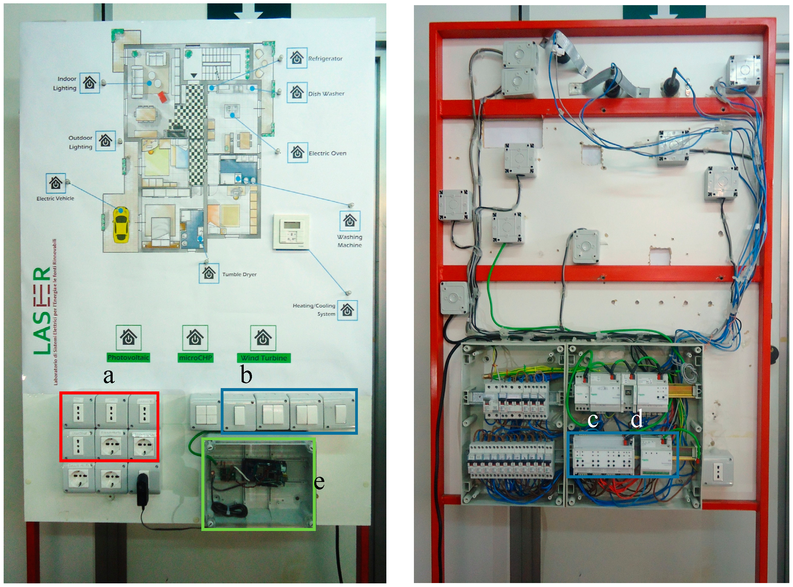
The front and rear sides of the above-mentioned demonstration panel of a residential unit are shown in Figure 11; the demonstration panel is connected to the 230 V/50 Hz utility grid and it is equipped with a real home automation system. The front side of the panel shows the plan of the house. Some icons with LED-lights link to appliances, meters, indoor and outdoor lights; when the LED lights are on, the corresponding peripheral is activated. Nine plugs are placed at the bottom left corner; six of these are smart plugs (see label a in Figure 11) and refer to an equal number of schedulable loads, the remaining three plugs refer to non-controllable loads. The on/off status of smart plugs can be manually set by means of the six smart buttons (see label b in Figure 11) equipped with a KNX interface device model n. MTN670804 (Schneider Electric, Rueil-Malmaison, France).

The rear side of the panel shows the electrical equipment, thermal-magnetic circuit breakers and the home automation system. At the pressure of a smart button, control frames are generated by the button itself and sent via the shielded twisted pair (STP) cable to a switch actuator (see label c in Figure 11) model n. REG-K/8×/16×/10 A; the actuator opens or closes the electrical circuit supplying the corresponding plug and load. A smart energy meter (see label d in Figure 11), model n. REG-k/3 × 230 V, measures the total electrical energy consumption.

Lastly, the label e in Figure 11 indicates a small case (width 240 mm, length 200 mm, depth 100 mm); both the low-EB and high-EB prototypes are mounted inside that case, as better illustrated in the following subsections.

4.2. The Aggregator

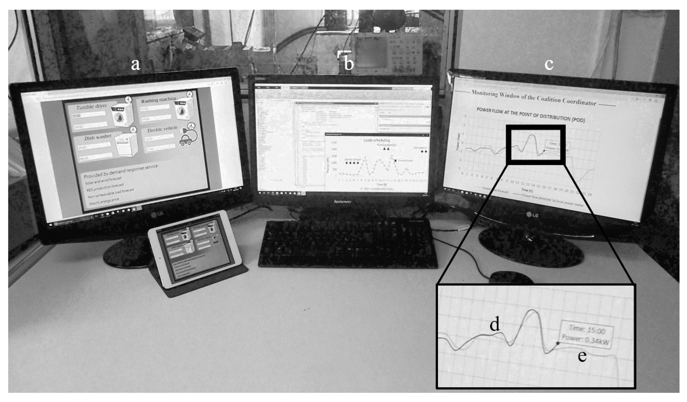
The customer coordinates the integrated community, it communicates to customers via the internet by means of the EBs so as to provide services such as the calculation of the optimal scheduling of customers’ loads. In the laboratory setup, the aggregator is a software, implemented in Matlab and running on a conventional personal computer. Figure 12 shows the aggregator’s graphic-user-interface (GUI) (see label a); the GUI is a conventional web page that the customer visits to upload his preferences regarding the operation of schedulable loads, i.e., the input parameters α_a and β_a of the prosumer problem. The aggregator solves the prosumer problem and calculates the optimal scheduling; Figure 12 also shows the Matlab software and the loads scheduling (see label b).

Furthermore, the aggregator receives and stores the energy consumption measurements returned by EBs; these data allow the aggregator to act as intermediary between the community and the distributed system operator. In particular, the aggregator executes the real-time calculation of power imbalances at the community level and implements strategies to provide ancillary services. With this in mind, Figure 12 (see label c) shows two lines where line d represents the daily forecast of the power flow at the point of delivery of a customer, while the line e represents the actual power flow as returned by the EB of the customer. It is worth noting that in Figure 12, line e stops at the last EB communication, i.e., at 3 p.m.

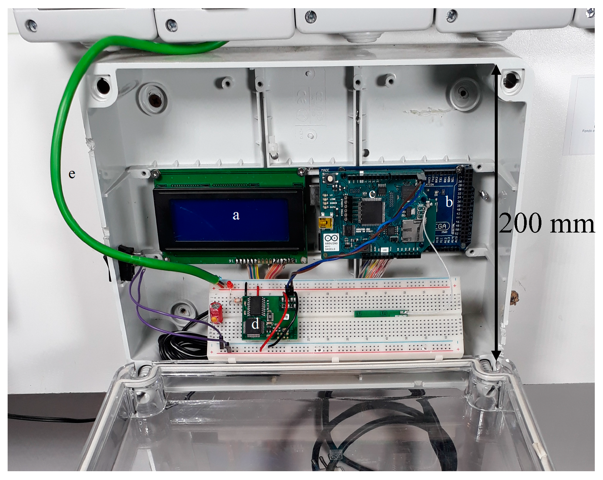
4.3. The Low-EB Prototype with Arduino

The prototype of the proposed energy box with a limited computing capacity is named low-EB and it mainly consists of: one liquid crystal display (LCD) with four lines and twenty characters per line, one Arduino Mega 2560, one WiFi shield for Arduino, one micro SD card and one sim Tapko KNX (TAPKO Technologies GmbH, Regensburg, Germany). Figure 13 illustrates the low-EB when installed into the case of the demonstration panel of Figure 11. The mission of the low-EB is exclusively to ask the aggregator for the load scheduling, i.e., the prosumer problem solution, and apply the scheduling. More precisely, the low-EB connects to the internet via a local router and synchronizes its internal clock to that provided by the National Institute of Meteorological Research [25]. Then, the low-EB sends a request to the aggregator for the load scheduling. 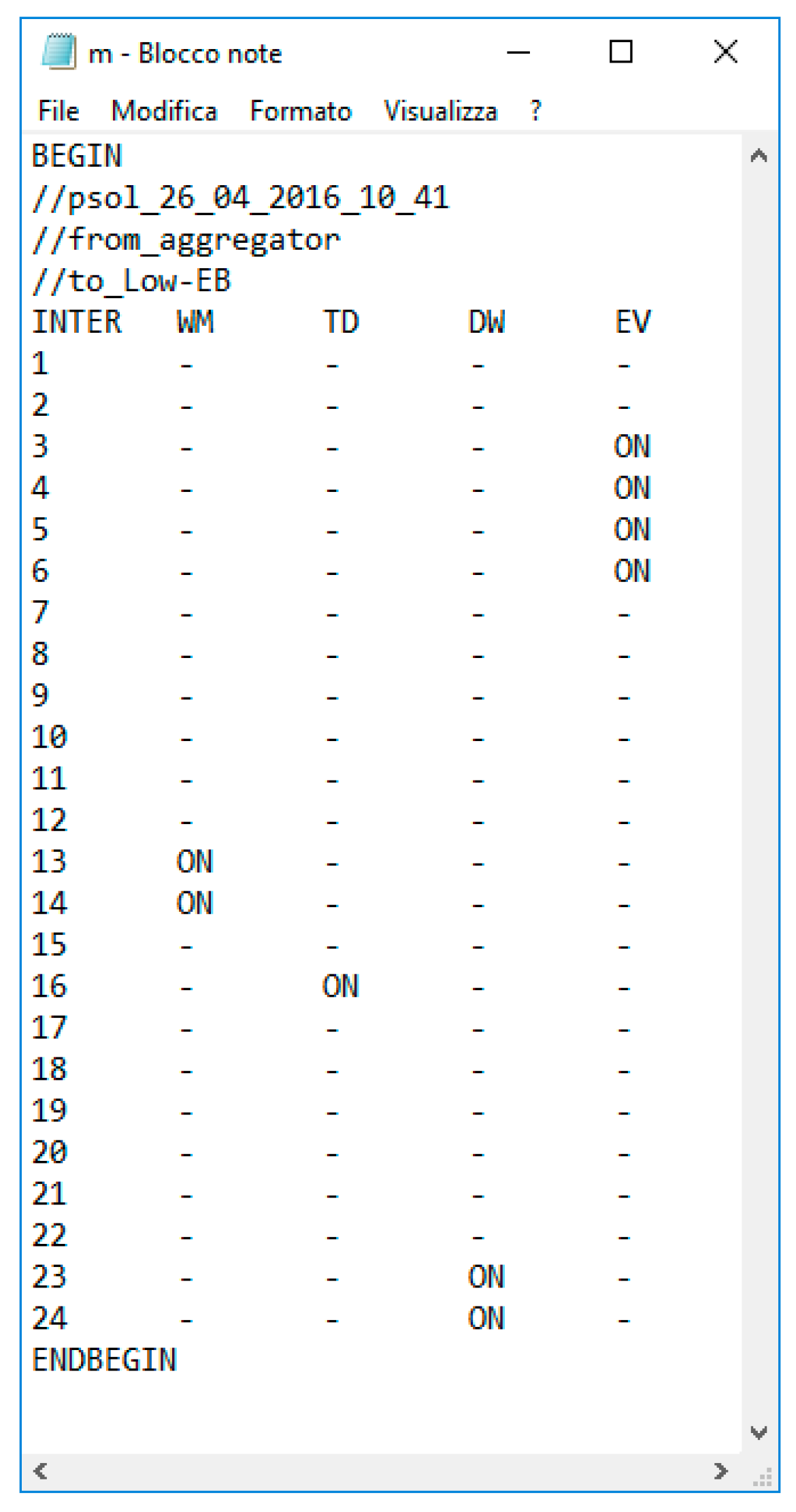The aggregator calculates the load scheduling in agreement with the customer’s preferences, i.e., the parameters α_a and β_a that the customer previously uploaded when he visited the aggregator’s GUI (see Figure 11, label a). The load scheduling is delivered to the low-EB in the form of a non-encrypted text file, as illustrated in Figure 14.

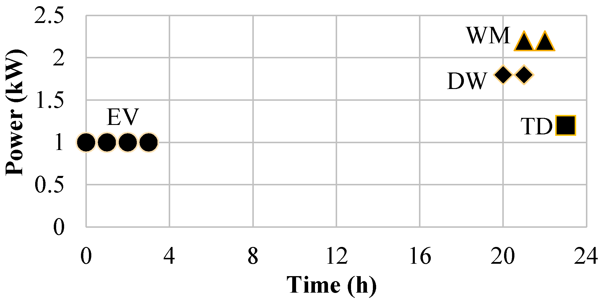
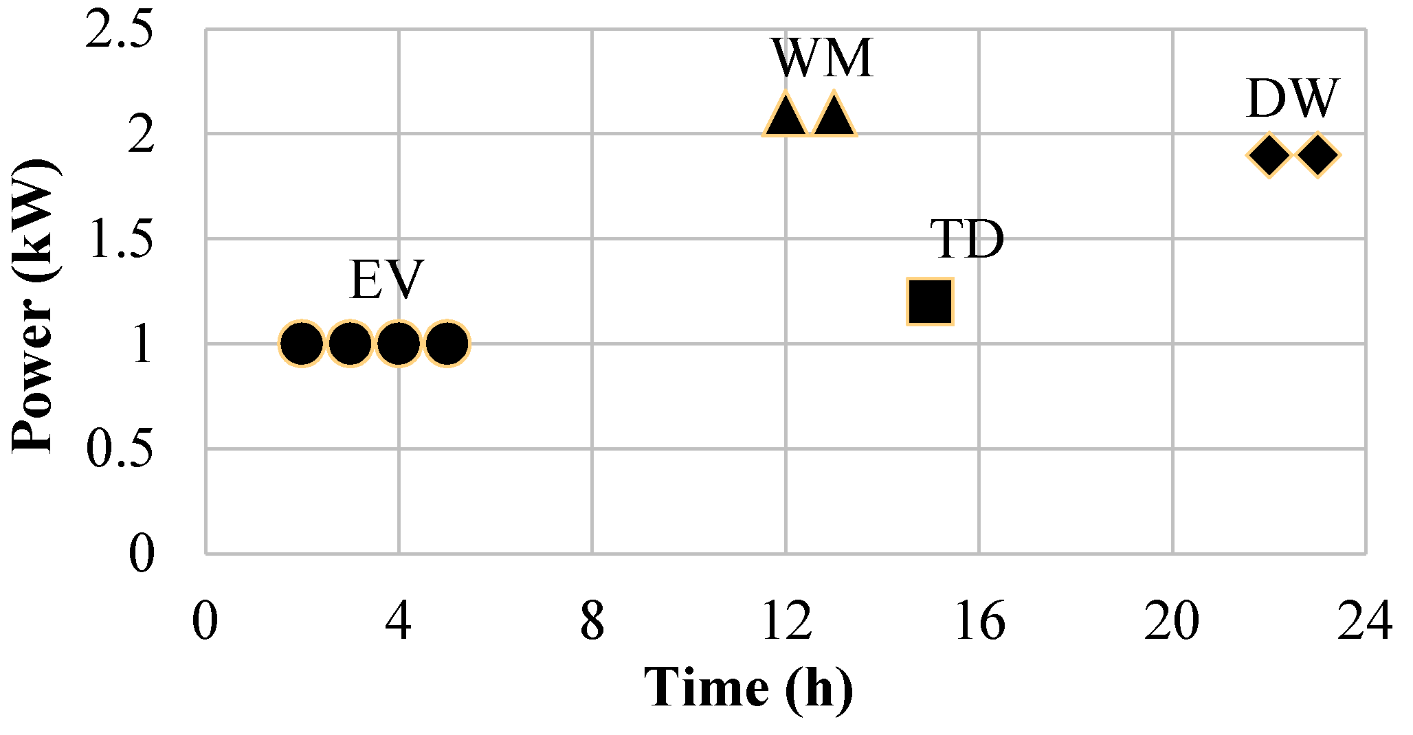
The text file starts with the reserved word BEGIN; three comments follow (a double slash “//” anticipate each comment). The first comment reports the name of the procedure psol that performed the load scheduling and the date/time when the scheduling has been calculated 26_04_2016_10_41; remaining comments report the sender aggregator and the recipient low-EB. These comments are definitely essential and useful because the low-EB may ask the aggregator for multiple solutions; for instance, the low-EB may ask for “emergency solutions” that is solutions where batteries are out of service or where the customer is suddenly disconnection from the utility grid. Therefore, the low-EB already has a loads scheduling to meet an emergency, pending the aggregator submitting an updated scheduling. Then, the text file reports the loads scheduling in the form of a table with five columns and 24 lines; the first column INTER relates to the daily hours from 1 to 23, while the remaining columns refer to the schedulable electrical loads (i.e., the washing machine WM, the tumble drier TD, the dishwasher DW, the electric vehicle EV). Each row is the hourly scheduling and it defines the state on/off of each schedulable load. For instance, the fourth row INTER = 4 indicates the time interval from 4:00 a.m. to 4:59 a.m.; for this interval the washing machine is off as the scheduling says “-” as well as the tumble drier and the dishwasher. On the contrary, the recharging of the batteries is running because the scheduling says “ON”.

At the beginning of every hour, the low-EB reads the corresponding row of the loads scheduling, it generates a set of control frames for each schedulable load, it converts control frames into analog signals and writes them to serial port pins where the sim Tapko KNX is connected. The sim Tapko, in turn, converts analog signals into control frames using the KNX protocol and writes them on the shielded twisted pair (STP) cable of the home automation system. Lastly, every five seconds the low-EB invokes the smart meter for the power measurement at the point of delivery, every minute it calculates the average value of the last 30 values, every 15 min it sends the last 15 mean values to the aggregator.

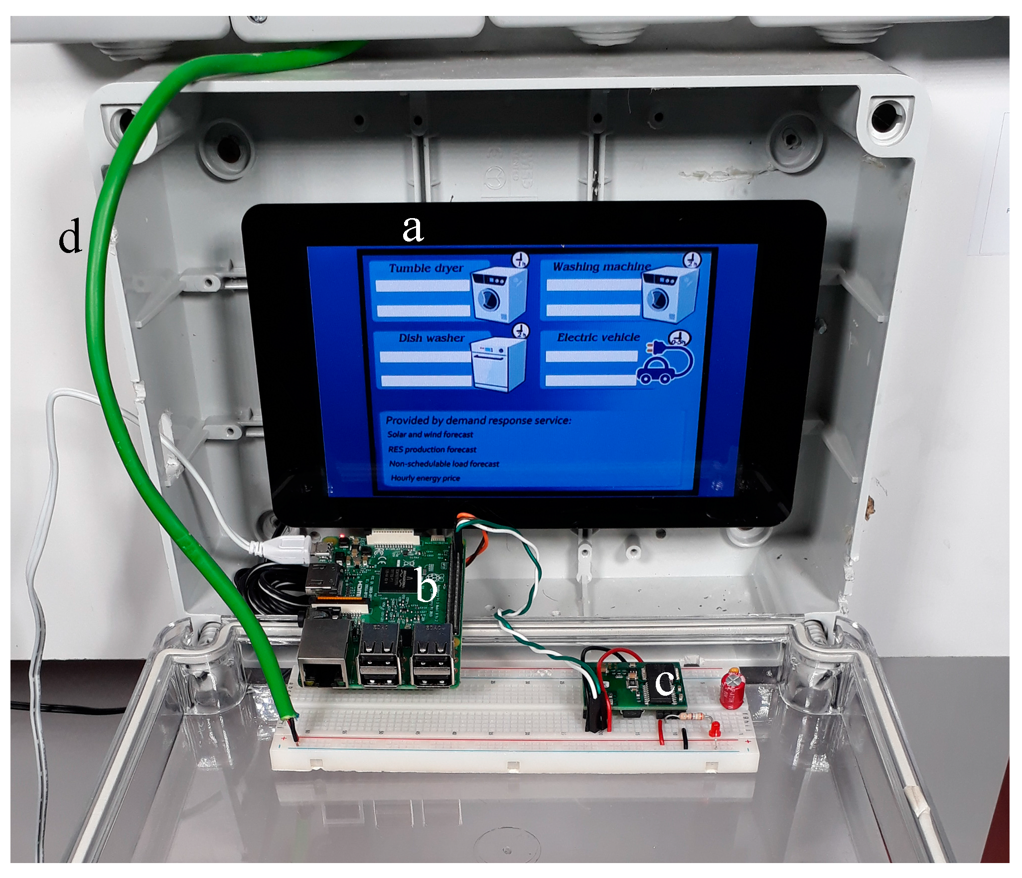
4.4. The High-EB Prototype Using Raspberry Pi3

The prototype of the proposed energy box with a higher computing capacity is named high-EB and it mainly consists of: a 7 inches touchscreen, one Raspberry Pi3 and sim Tapko KNX. Figure 15 illustrates the High-EB when installed into the case of the demonstration panel of Figure 11. The high-EB performs the same functions performed by the low-EB and, in addition, it is capable to self-calculate the optimal scheduling of consumer’s loads. At this scope, the high-EB facilitates the customer in indicating their preferences, α_a and β_a, because the aggregator’s GUI (see Figure 12 label a) now locally runs on the Apache web server application installed on the Raspberry Pi3 (see Figure 15 label a). The high-EB communicates with the aggregator and asks for services such as the hourly electricity prices and the hourly PV-wind generation forecast for the customer’s site. The high-EB uses the customer’s preferences, prices and forecasts to calculate the optimal loads scheduling; the high-EB hourly generates and writes control frames on the STP cable using the sim Tapko KNX in order to apply the loads scheduling.

As well as the low-EB, every five seconds the high-EB carries out a reconnaissance on the system’s power consumption; in particular, it invokes the smart meter for the power measurement at the point of delivery and every 15 min it sends the last 15 mean values to the aggregator.

In order to allow the high-EB to self-calculate the loads scheduling, we programmed the prosumer problem into the Raspberry Pi3 using the development environment named Eclipse for Java programming. In order to solve the prosumer problem, we used the IBM ILOG CPLEX Optimization Studio solver (CPLEX); such a solver uses the simplex method, it runs on Linux (i.e., the Raspberry Pi3 operative system) and it solves the prosumer problem within 10–15 s.

5. Conclusions

This paper proposed an energy box (EB) as a viable solution to the challenge of the communication between a consumer and an aggregator; indeed, the proposed EB communicates with the aggregator’s IT platform and requires access to an application, service or system. For instance, the proposed EB uploads the user’s preferences to obtain optimal loads scheduling and savings on the electricity bill. Furthermore, the proposed EB uploads power/voltage/current measurements to obtain reports and statistics. The proposed EB is also a viable solution to the challenge of the interaction between an EB and home energy management systems (HEMSs); indeed, the proposed EB overcomes the problem of interaction because it directly communicates with all peripherals of the home automation system, bypassing the HEMS. In particular, the proposed EB self-generates the control frames to turn on/off a load or to acquire a measurement from a smart meter; then, the EB sends these frames to loads and smart meters via the physical media for the communication of the home automation system.

The paper also illustrated two prototypes of the proposed EB to have a clear overview of management and material requirements, as well as of cost-effectiveness; both prototypes were tested in the laboratory using a real home automation system. The two prototypes are relevantly cost-effective and effectively serve prosumers and prosumages in autonomous demand response program in cloud-based architectures. The first prototype has a limited calculation capability and a very low cost (low-EB), the second prototype has a higher cost but also a higher capacity for solving calculation problems (high-EB). The low-EB communicates with the aggregator over the internet to exchange data and submit service requests; in particular, the low-EB asks and receives the optimal scheduling of the consumer’s loads from the aggregator. The low-EB applies the load scheduling by sending the on/off commands directly to the peripherals of the home automation system, bypassing the HEMS. The high-EB performs the same functions as the low-EB and, in addition, it is capable to self-calculate the optimal scheduling of the consumer’s loads. The low-EB uses on an Arduino MEGA 2560, whereas the high-EB uses a Raspberry Pi3.

Future work and research will focus on the relationship between the goals at the aggregator’s level and the preferences at the customers’ level; at this scope, many field measurements are necessary. With this in mind, we are already involved in a project on power cloud and distributed energy storage systems; we plan to build a certain number of EBs and give them to real customers. In this way, an appropriate quantity of data, information and measurements will be available to evaluate the relationship between goals at the aggregator’s and customer’s levels.