A Comparison Analysis of BLE-Based Algorithms for Localization in Industrial Environments

Abstract

Proximity beacons are small, low-power devices capable of transmitting information at a limited distance via Bluetooth low energy protocol. These beacons are typically used to broadcast small amounts of location-dependent data (e.g., advertisements) or to detect nearby objects. However, researchers have shown that beacons can also be used for indoor localization converting the received signal strength indication (RSSI) to distance information. In this work, we study the effectiveness of proximity beacons for accurately locating objects within a manufacturing plant by performing extensive experiments in a real industrial environment. To this purpose, we compare localization algorithms based either on trilateration or environment fingerprinting combined with a machine-learning based regressor (k-nearest neighbors, support-vector machines, or multi-layer perceptron). Each algorithm is analyzed in two different types of industrial environments. For each environment, various configurations are explored, where a configuration is characterized by the number of beacons per square meter and the density of fingerprint points. In addition, the fingerprinting approach is based on a preliminary site characterization; it may lead to location errors in the presence of environment variations (e.g., movements of large objects). For this reason, the robustness of fingerprinting algorithms against such variations is also assessed. Our results show that fingerprint solutions outperform trilateration, showing also a good resilience to environmental variations. Given the similar error obtained by all three fingerprint approaches, we conclude that k-NN is the preferable algorithm due to its simple deployment and low number of hyper-parameters.

1. Introduction

In recent years, similarly to what is happening in cities and public spaces, smart and connected objects are increasingly being deployed also in industrial environments. One of the effects of the development of this so-called smart industry (also known as Industry 4.0) is an increase in the number and type of automated vehicles that move in industrial environments. In this context, indoor localization systems become important to improve logistics effectiveness and productiveness. In many industrial sectors, the quick and automatic localization of goods (components, instruments, partial assemblies, etc.) in large environments would provide a critical production speed up. For instance, a critical problem in the automotive industry is the quick localization of partially assembled vehicles which are temporarily removed from the pipeline and placed in large warehouses, e.g., while waiting for the availability of some of the parts required for their completion.

In literature, several existing technologies like global positioning system (GPS) [1], Wi-Fi [2], and Bluetooth [3] are adapted to provide indoor localization services in domestic environments. While GPS performance indoor is poor [1], Wi-Fi and Bluetooth show promising results, with the latter being particularly interesting due to its low cost and energy consumption features [4].

The use of Wi-Fi for indoor positioning is well established and is known to provide errors in the order of few meters [5]. However, the requirements in terms of topological distribution, number of Wi-Fi access points associated with the costs and power consumption make this solution unfeasible without a consistent retrofitting which is often undesirable in existing industrial plants (e.g., make power outlets available at deployment points).

Bluetooth low-energy (BLE) uses the same frequency of Wi-Fi ($2.4$ GHz) but is designed as a short range energy-efficient communication protocol, allowing compatible devices to communicate through short messages with minimal overhead [6]. Thanks to these features, BLE-compatible devices can transmit periodic messages for years within a single cycle of a small form-factor battery [7], thus being perfectly suited for easy installation in any environment.

BLE-based localization is typically performed by installing a set of proximity beacons (i.e., BLE transmitters) at known locations. Receivers extract the RSSI (which is a proxy of the distance from the sender) from the nearest beacons and use these values to predict their own position [8].

In general, BLE-based localization algorithms can be split in two categories: distance-based and fingerprinting-based [9]. Distance-based algorithms directly translate RSSI values into position coordinates for the object being localized. These methods require that at least three RSSI measurements from nearby beacons are available, and apply either trilateration or min-max to transform these measurements into position estimates [10]. In contrast, fingerprinting-based algorithms exploit a vector of RSSI measurements in known fingerprint positions to create a so-called reference fingerprint map (RFM). Then, a machine-learning regressor is fed with the RFM data to build an association rule between new RSSI measurements and their corresponding position estimates [11].

Although these techniques have been proven effective in domestic settings, smart industry environments pose several new challenges that need to be addressed: the areas where objects have to be localized are much larger than in the domestic case, and they constitute a harsh environment for BLE-based localization, due to the presence of large metal objects (robots, carts, etc.) causing signal interference, multi-path propagation and shadowing. Despite the vast literature on BLE-based localization, very few works perform detailed comparisons between different algorithms under the same experimental conditions (i.e., target environment, type and number of beacons and receivers, etc.). In particular, to the best of our knowledge, no one focuses on applying these methods in real industrial environments.

In this work, we perform such comparison considering two real industrial settings (i.e., a shed and a workshop). We evaluate the effectiveness of several state-of-the-art algorithms (both distance-based and fingerprinting-based) under varying experimental parameters, changing the number of installed beacons and the density of the RFM. Moreover, we assess the robustness of fingerprint-based algorithms to variations in the environment and to random noise.

Our goal is to assess the feasibility of indoor localization in industrial environments using commercial off-the-shelf BLE transmitters and receivers, due to their low cost, ready availability and ease of installation and usage. The experiments performed are consequently tailored for this target, and are based on commercial devices and protocols currently available in the market.

Similarly, the goal of this paper is to test the effectiveness of state-of-the-art localization algorithms for BLE localization in an industrial scenario. Therefore, we do not aim at designing a new specialized algorithm for this task, and we just optimize the hyper-parameters of existing solutions to the best values for our target.

Our results confirm that fingerprinting-based methods reduce the positioning error compared to distance-based methods, even in an industrial setting. However, we could not identify a clear winner among the three fingerprinting-based algorithms considered in our experiments, as they all perform similarly both in terms of positioning error and of computational complexity. Therefore, we base our final selection on simplicity and flexibility, which leads us to choose k-NN, as explained below.

The rest of this paper is organized as follows. Section 2 reviews relevant literature solutions. Section 3 presents the localization algorithms analyzed in this study and Section 4 discusses the experimental results. Finally, Section 5 offers our concluding remarks.

2. Background and Related Work

Indoor localization methods based on the received signal strength indication (RSSI) from BLE devices have become mainstream thanks to their low cost, wide coverage, and simple hardware required. In comparison, more accurate alternatives such as those based on the angle of arrival (AOA) or on the time of arrival (TOA) require significantly more expensive hardware, since they rely either on an array of BLE antennas or on a very accurate synchronization between the transmitter and receiver [12].

The RSSI is a measurement of the power present in a received radio signal. It is typically computed as the ratio between the received signal power and the transmission power, which is a known value set by manufacturer, and attached to each packet sent by the beacons [13]. As mentioned above, RSSI is generally used for two types of localization methods: distance-based methods [10] and fingerprint-based methods [14]. While the former try to directly convert RSSI values to distances, the latter use a RFM to build a model that associates new RSSI measurements to a position.

The two main distance-based methods are trilateration [11] and min-max [15]. Both convert RSSI values to distances between beacon and localized device using the quadratic decay law of power with respect to distance. Trilateration determines the location of an object combining measurements from three spatially-separated known locations (beacons). The position of the device is obtained as the intersection of the three circumferences having the location of one beacon as the center and the computed distance as radius [10]. The min-max algorithm constructs a square bounding box around each beacon using its known coordinates as center and two times the distance from the target as side length of the box. Next, the intersection of three boxes is computed selecting the min-max coordinates. This approach is computationally simpler than trilateration, but it is also more prone to errors.

In both cases, the error obtained by distance-based methods is influenced by the number of installed beacons and in particular by their density (number of beacons per square meter). Moreover, trilateration and min-max are influenced by multi-paths and fading. Multi-paths are propagation phenomena that occur when radio signals reach the receiving antenna by two or more paths. Multi-path propagation causes constructive or destructive interference and phase shifting of the signal, which in turn can vary the measured RSSI. Fading is a more generic variation of the attenuation rate of a signal due to obstacles, frequency disturbances or obstacles, which can result in a loss of signal power.

Several works use distance-based positioning with BLE beacons in various domestic or public environments. In [16], the authors use trilateration in a hall of 7 m × 5 m where the maximum distance from the beacons to the target is less than 9 m. Despite the small size of the environment, their experiments using three beacons produce an average error of 2.766 m. In [17], the authors optimize the trilateration algorithm applying a Kalman filter to reduce noise in the RSSI. Park et al. [18] calculate the distance using the RSSI and then they refine the result applying two Kalman filters to reduce the error. Using six beacons in a polygonal living room (8.5 m × 13 m), they obtain an average error of 1.77 m. In [19], the authors use the min-max algorithm to obtain the object position in three environments: a classroom and two construction sites. The classroom has size 7 m × 6.4 m and the distance between beacons varies from 3 m to 4.8 m; the average error obtained is 1.55 m. The two construction sites have the same size (6.3 m × 5.1 m) and are tested with six and three beacons respectively, positioned with a spacing ranging from 1 m to 3.4 m; the average errors obtained are 1.22 m and 2.58 m.

Fingerprinting refers to the type of algorithms that estimate the location of an object exploiting previously recorded data at known positions. Therefore, RSSI-based location fingerprinting requires a preliminary set-up stage. An inspection of the environment is performed to select reasonable data collection points to create the RFM. The coordinates of these points and the corresponding RSSI values from nearby beacons are collected. Then, these data are used to build a model that associates a new RSSI measurement to its corresponding location. Several types of models, typically based on machine-learning are considered in literature. Therefore, fingerprinting allows for partially accounting for multi-paths and fading due to fixed (not moving) elements of the environment, as these effects are measured also in the “training” RFM data.

In [20], the authors use the k-nearest neighbors (k-NN) algorithm with $k=8$ and different number of fingerprints points in a living room of 6.66 m × 5.36 m. With a RFM of 50 points, they obtain an average localization error of 1.03 m, while with an RFM of just eight points they obtain an average error of 1.91 m. Dierna and Machì in [21] an experiment with 31 beacons in a museum of 670 m${}^2$ using two different sampling densities to create the RFM and a k-NN model with $k=3$. In a first experiment, the density is varied from $0.7$ reference points per square meter in museum halls to one point every four square meters in the courtyard (224 total RFM points). The authors also experiment with averaging RSSI measurements over multiple samples, obtaining an error that varies from 1.72 m (1 sample) to 1.28 m (10 samples). Then, the authors try to increase the RFM sampling density in proximity of structural points, obtaining 239 total points and reducing the error to 1.70 m (without averaging). In [22], authors develop an Iterative Weighted k-NN (IW-kNN) for fingerprinting-based localization. They select $k=4$ and use 10 beacons in a test room of 18.8 m × 12.6 m, obtaining an average error of 2.52 m. In [23], the author propose a k-NN with $k=1$ in an small office room. Using 20 beacons and an RFM of 120 points, the average error obtained is 1.9 m.

Other studies map the localization problem to a regression or classification using support vector machines (SVM) or neural networks (multi-layer perceptrons—MLPs). In [24], the authors test different configurations of a Multi-Layer Perceptrons in two different locations, a room of 4 m × 4 m and a 36 m-long corridor. In the test room, they use four beacons and 16 RFM points, obtaining an average error of 2.48 m. In the test corridor, nine beacons and 36 RFM points yield an average error of 1.25 m. In [25], the authors use an SVM in a living room of 3.53 m × 8.09 m divided in six zones, with two beacons placed in the middle of the room, equidistant from the walls. A set of RSSI values are taken in different zones of the room and out of it to test the algorithm. The SVM shows an accuracy of $88.54\%$ in classifying the zone.

Both distance-based and fingerprint-based localization algorithms can be applied either directly on the raw RSSI values measured at the receiver, or after extracting some higher-level features by aggregating or processing those raw values.

Table 1. Summary table including relevant works on indoor localization based on Bluetooth low-energy (BLE) received signal strength indication (RSSI) and the corresponding feature extraction methods.

Authors	Feature Extraction
Varshney et al. [4]	None/Not Mentioned
Chintalapudi et al. [5]	None/Not Mentioned
Čabarkapa et al. [9]	None/Not Mentioned
Er Rida et al. [10]	Sample Average
Kriz et al. [11]	Sample Average
Cho et al. [12]	None/Not Mentioned
Subhan et al. [14]	Sample Average
Palumbo et al. [15]	Sample Average (removing outliers)
Rattanalert et al. [26]	None/Not Mentioned
Grzechca et al. [16]	Sample Average, Moving Average, Sample Median, etc.
Ibrahim et al. [17]	None/Not Mentioned
Park et al. [18]	Sample Average
Luo et al. [19]	None/Not Mentioned
Daniş et al. [20]	Entire Histogram
Dierna et al. [21]	Sample Average
Peng et al. [22]	Sample Average (removing outliers)
Larsson [23]	Sample Average
Mazan et al. [24]	Sample Maximum
Rodríguez-Damián et al. [25]	None/Not Mentioned
Faragher et al. [27]	None/Not Mentioned
Faragher et al. [28]	None/Not Mentioned
Bailey et al. [29]	None/Not Mentioned

summarizes the feature extraction methods adopted in the relevant literature works on this problem.

As shown in the table, many works [4,5,9,12,17,19,25,26,27,28,29] do not perform any feature extraction and work directly on raw RSSI data. Another common solution [10,11,14,18,21,23] is to use as feature the average of RSSI measures over a short interval of time (from a few seconds to some minutes) for noise rejection. Other authors [15,22] also use the average RSSI over a time window, but remove outliers before computing it. Mazan et al. [24] use the RSSI sample maximum rather than the average, while Grzechca et al. [16] consider several different summary statistics as possible features for localization (sample average, median, etc.). Eventually, however, they determine that the average/moving average is the feature that yields the best results. Lastly, Daniş et al. [20] store the entire histogram of RSSI measurements over a time interval, where each bin of the histogram could be considered as a different feature. However, they do not use these features to perform localization. Rather, they use them to generate a dense RFM from a sparse one.

According to literature [27], there are many factors affecting the accuracy of BLE-based localization. When a receiver moves through the environment, the RSSI signal can vary abruptly due to the presence of walls and objects. The signal can penetrate differently through different materials and interact with objects as it moves along different paths through the environment. Furthermore, fingerprinting schemes require regular review to ensure the accuracy of the map. If environmental changes (e.g., movements of large objects) occur, fingerprinting methods performances can degrade drastically. More specifically, the positions of furniture elements, the density of people and even the positions of walls and partitions can influence the measurements. In [28], the authors analyze the problem of multi-paths and possible mitigation schemes when the beacon signals are transmitted using different frequencies (2402 MHz, 2426 MHz, and 2480 MHz). They also verify that positioning accuracy increases with the number of beacons measured in each fingerprint point, up to a threshold of around 6–8, beyond which there is no quantifiable improvement.

As mentioned in Section 1, while all these factors are relevant even in the case of a domestic or public space, their impact is expected to increase in an industrial scenario, due to the larger size of environments and the abundance of reflecting materials such as metal. However, none of the aforementioned papers compared different BLE-based localization algorithms in the context of a Smart Industry application, which is exactly the main contribution of this work.

3. Localization Algorithms

In this work, we considered one distance-based algorithm (Trilateration) and three fingerprint-based algorithms (k-NN, SVM, MLP). These algorithms have been selected as those that provide the most consistent results across different types environments in literature (see Section 2). All considered fingerprint-based algorithms could be used for either classification or regression. The former solution could be used when the goal is simply to identify the area (e.g., room) where the target object is located, whereas the latter approach is needed to obtain precise coordinates. Consequently, we use all three fingerprint-based algorithms in regression mode. In the following, we describe each algorithm in detail, focusing in particular on the hyper-parameters settings used in our experiments.

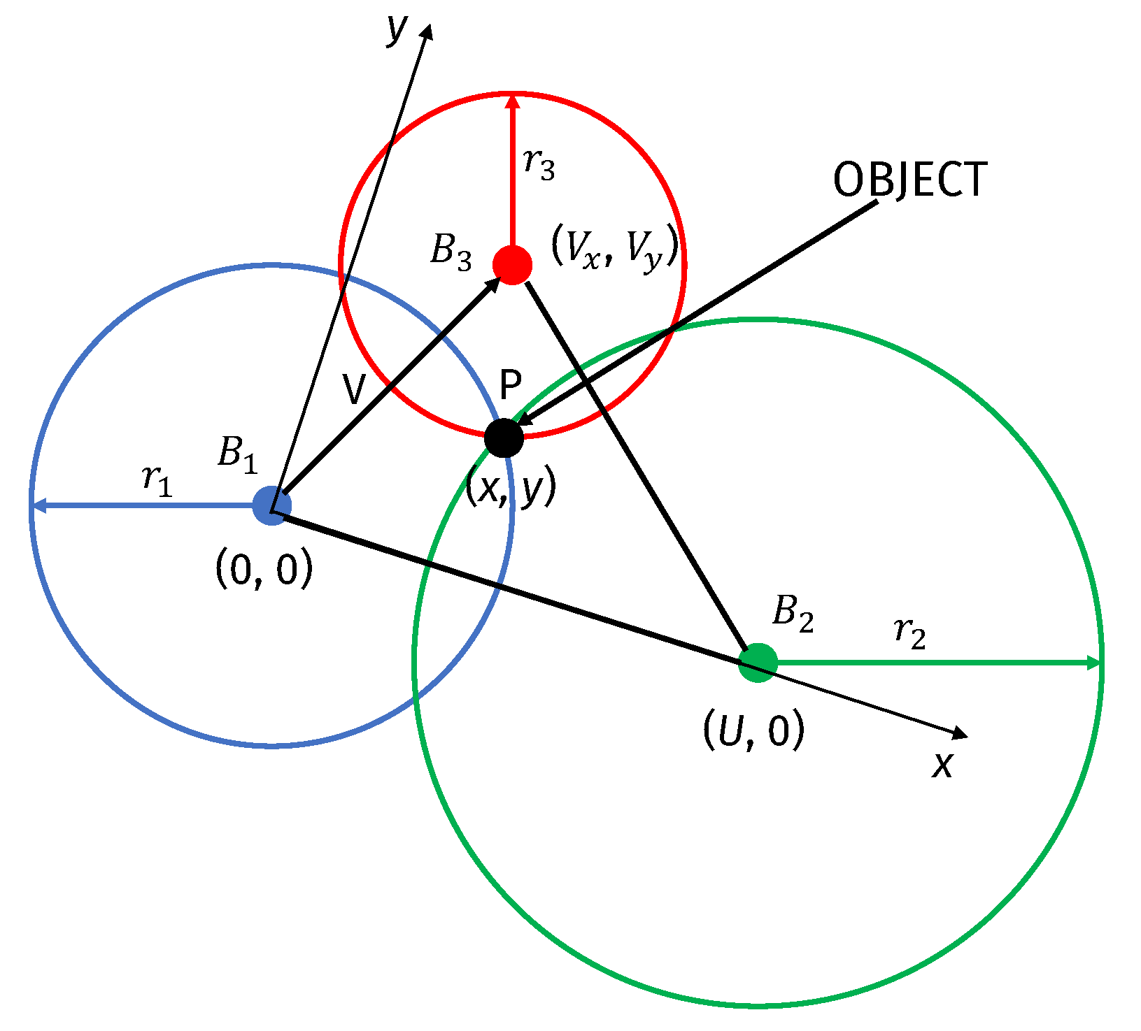
The trilateration algorithm (see Figure 1) is a sophisticated version of triangulation which calculates the distance from the target object directly, rather than indirectly through the angles. Data from a single beacon provide a general location of a point within a circle area. Adding data from a second beacon allows for reducing the plausible area to the overlap region of two circles, while adding data from a third beacon reduces it to a point. In the figure, U is the known distance between beacon 1 ($B_1$) and beacon 2 ($B_2$), while $V_x$ and $V_y$ are the coordinates of beacon 3 ($B_3$) with respect to $B_1$. The radii of the three circles, obtained from RSSI measurements are $r_1$, $r_2$, and $r_3$. With this notation, the coordinates of the object P in a 2D space are calculated using the following equations:

$$\begin{array}{cc}\hfill V^2& =V_x^2+V_y^2,\hfill \\ \hfill x& =\frac{r_1^2-r_2^2+U^2}{2U},\hfill \\ \hfill y& =\frac{r_1^2-r_3^2+V^2-2V_{x}x}{2V_y}.\hfill \end{array}$$

The k-Nearest Neighbors algorithm (k-NN) is a non-parametric supervised learning method that can be used for both regression and classification [29]. When k-NN is used for regression, the output of the algorithm is the property value of the object (i.e., its position) calculated as a weighted average of the values of its k nearest neighbors, where k is the main hyper-parameter of the algorithm. K-NN does not require a proper training, as it just requires storing the RSSI values and corresponding coordinates for the training data. At inference time, the k nearest neighbors of a new sample are simply identified evaluating a distance metric between its RSSI measurements and those of all training data.

In our work, we tested different values of k and selected the one that yielded the lowest median error on the test data set. We obtained that the optimal value of k did not depend on the density of beacons present in the environment. However, our tests only included either three or four beacons in two different environments, hence the optimal value may change in a different scenario. Nonetheless, finding the best value of k is a straightforward process if the number of test points is not extremely large, since this is the only hyper-parameter of the algorithm. The value of k used in our experiments is reported in Section 4.1.

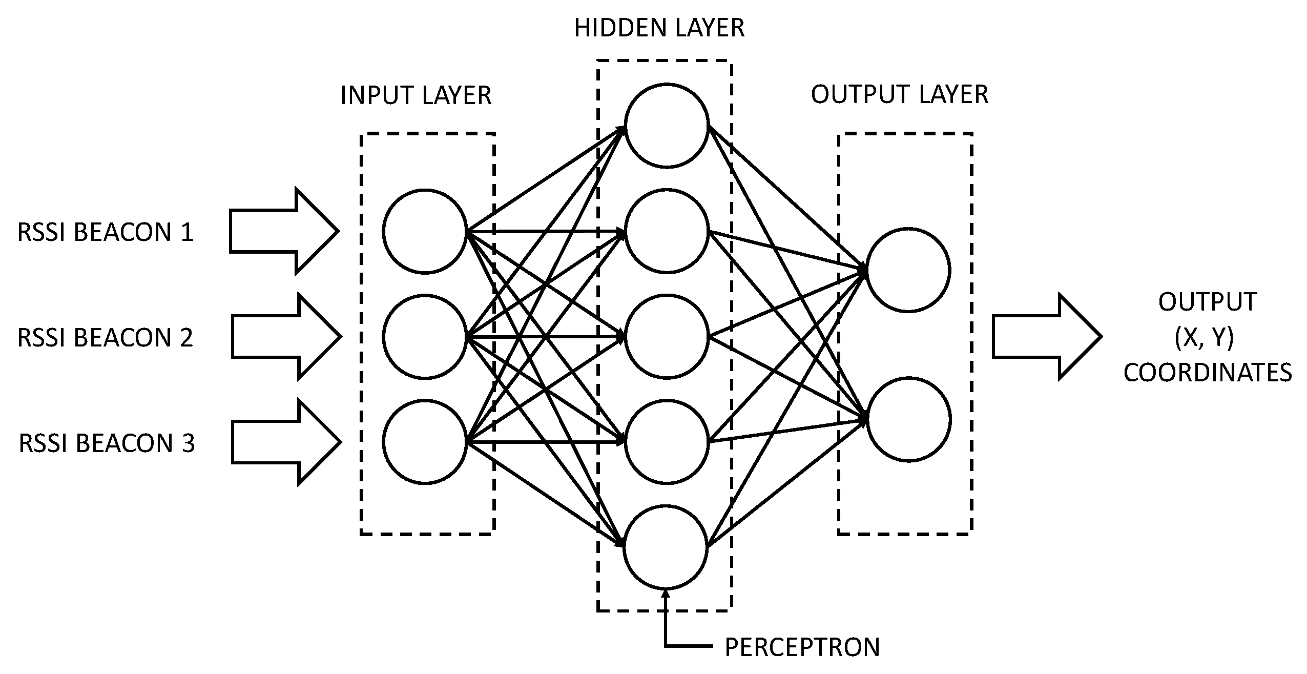
The multi-layer perceptron (MLP) is a type of feed-forward artificial neural network used in supervised regression and classification tasks [30]. As shown in Figure 2, an MLP consists typically of three or more layers of neurons: (i) an input layer, (ii) an output layer, and one or (iii) more hidden layers. MLPs are trained using backpropagation and exploit nonlinear activation functions (rectified linear unit—ReLU or sigmoid functions) in the hidden and output layers to learn complex input/output relationships.

In our work, the number of neurons in the input layer is equal to the number of beacons whose RSSI measurements are recorded (which varies among different environments and experiments), while the number of output neurons is fixed to 2, i.e., the predicted $(x,y)$ coordinates of the target object. Concerning the hidden layers, we tried different combinations of number of layers and neurons. The exact type and number of layers used in our experiments are reported in Section 4.1.

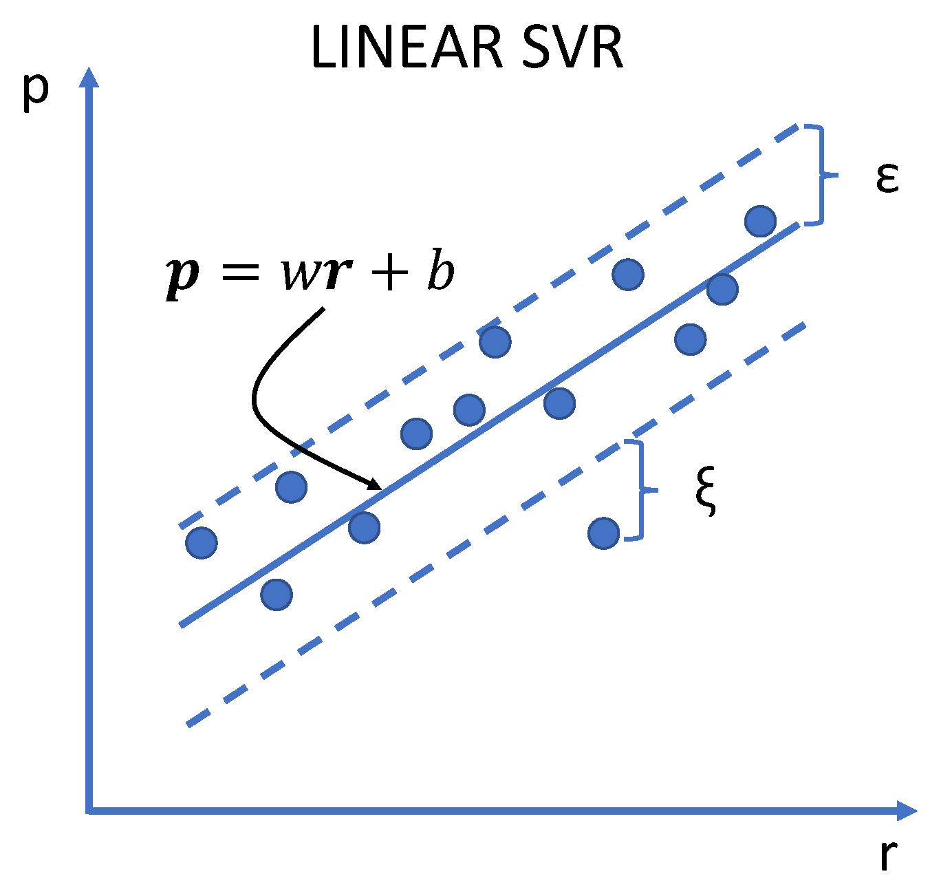
Lastly, support–vector machines (SVM) can also be used for supervised classification and regression [30]. When used for regression, SVMs are more properly called support–vector regressors (SVRs) and are trained to predict the output variables with a given margin of tolerance, called $\epsilon$. In its basic form, the SVR training algorithm finds a hyperplane that maximizes the number of samples that fall within the margin (see Figure 3). In practice, this is a transformation of the type:

$$\mathbf{p}=w\mathbf{r}+b,$$

(1)

where $\mathbf{r}$ is the vector of RSSI values measured from the beacons, $\mathbf{p}$ is the corresponding vector of coordinates (x, y) of the object, and w and b are a matrix and a vector of weights, which are optimized to maximize the number of training samples that fall within the margin. Nonlinear relationships are dealt with by projecting the input variables using a kernel function. For instance, the common Radial Basis Function (RBF) kernel transforms the input $\mathbf{r}$ onto:

$$K(\mathbf{r}-{\mathbf{r}}^{\prime })=exp(-\gamma \parallel \mathbf{r}-{\mathbf{r}}^{\prime }{\parallel }^2),$$

(2)

where $\gamma$ is a hyper-parameter used to optimize the hyperplane and $\parallel \mathbf{r}-{\mathbf{r}}^{\prime }{\parallel }^2$ is the squared Euclidean distance between two input samples ($\mathbf{r}$ and ${\mathbf{r}}^{\prime }$).

For a sufficiently complex problem, some data will inevitably fall outside of the tolerance margin (see Figure 3). SVR training tries to minimize the total distance of these points from the margin ($\xi$) including a penalization term $C\sum \xi$ to the objective function. The hyper-parameter C is used to weigh the importance of these outliers.

In our work, we used a grid search to find the best combination of hyper-parameters for an SVR. Specifically, we varied the kernel function, the kernel coefficient $\gamma$ (only when using a RBF kernel), the boundary limit $\epsilon$ and the penalty parameter C. We considered linear and RBF kernels, whereas $\gamma$ was varied in the interval [0.01–0.08], $\epsilon$ in [0.02–0.08], and C in [1–100]. The exact kernel functions and the optimal values of the parameters found in our experiments are reported in Section 4.1.

4. Results and Discussion

4.1. Experimental Setup

In our experimental setup, we used up to four beacons as BLE transmitters. As mentioned in Section 1, we wanted to focus on off-the-shelf BLE-based devices that could be bought on the market today at a low cost to implement indoor localization in industrial environments. Specifically, we selected Estimote beacons [31] because of their low cost and long battery lifetime. These devices adopt the Apple proprietary “iBeacon” protocol [32] to broadcast information packets over BLE. Each packet includes a universally unique identifier (UUID) of the beacon and an indication of the nominal transmitted power at 1 m from the device, which is needed to convert RSSI measurements into distances.

As a target device to be localized, we used a Raspberry Pi 3 B (quad-core ARM [email protected] GHz) with its on-board Bluetooth receiver. All localization algorithms have been implemented in Python using the sklearn package [33]. In order to improve the correlation between the measurements collected when building the RFM and those exploited to localize the device, the Raspberry Pi has been used for both tasks. The localization algorithms described in Section 3 have been compared in two industrial environments:

• Environment A is an industrial shed of 100 m${}^2$, with a 9 m high ceiling. The walls are partly masonry partly metal, with a doorway of 4 m${}^2$ on a side. The area is partially occupied by pallets and building materials of different types.
• Environment B is an industrial workshop of 288 m${}^2$ with a 10 m high ceiling. The area contains electronic and mechanics equipment, computers, and metal structures and was continuously in use by workers during our experiments. The walls are partly masonry partly glass.

Beacons have been positioned as equidistant as possible from each other, given the restrictions caused by obstacles in the two environments. When using four beacons, the minimum distance between them was ≈3.9 m and ≈7.7 m for Environment A and Environment B, respectively. Notice that a simple localization method based on proximity (i.e., one that simply detects the area of the environment based on the beacon that generates the strongest RSSI) would incur an error that is always greater than half of these distances (i.e., >1.85 m and >3.85 m respectively for the two Environments). Therefore, these half-distances represent a sort of lower bound on the acceptable performance of any localization algorithm that exploits more than one beacon, such as trilateration and fingerprint-based ones.

Fingerprint methods have been tested with different densities of points in the RFM. Specifically, for both environments, we considered three grids of equidistant points with a distance between adjacent points of 0.5 m, 1 m and 2 m, respectively. RFM points have been collected whenever the corresponding location was not obstructed by furniture or other obstacles. This gave us a total of 192 RSSI values for training and 31 for testing in Environment A, while, in Environment B, we measured 293 RSSI points for training and 50 for testing.

In accordance with many literature papers on indoor localization using BLE RSSI [10,11,14,15,16,18,21,22,23], we used a simple yet effective “feature extraction” method. Specifically, rather than using raw RSSI measurements to perform localization, we averaged the measurements over an interval of time to partially filter noise. For training measurements, we averaged the RSSI over intervals of 1 min. Testing measurements have been performed for intervals of 20 s to avoid increasing too much the time required to obtain an estimate of the position. In both training and testing measurements, the Raspberry Pi was randomly oriented, to simulate a realistic localization scenario. The ground truth positions of training and testing points have been measured using a professional meter.

For the k-NN algorithm, we tested different values of k and we obtained the best performance using $k=3$. For the MLP, the lowest error was obtained with a model including three hidden layers composed of 8, 8, and 6 neurons, respectively, and using ReLU activation functions. For the SVR, the lowest median localization error was obtained with the RBF kernel, $\gamma =0.01$, $\epsilon =0.02$ and $C=1$.

4.2. Trilateration

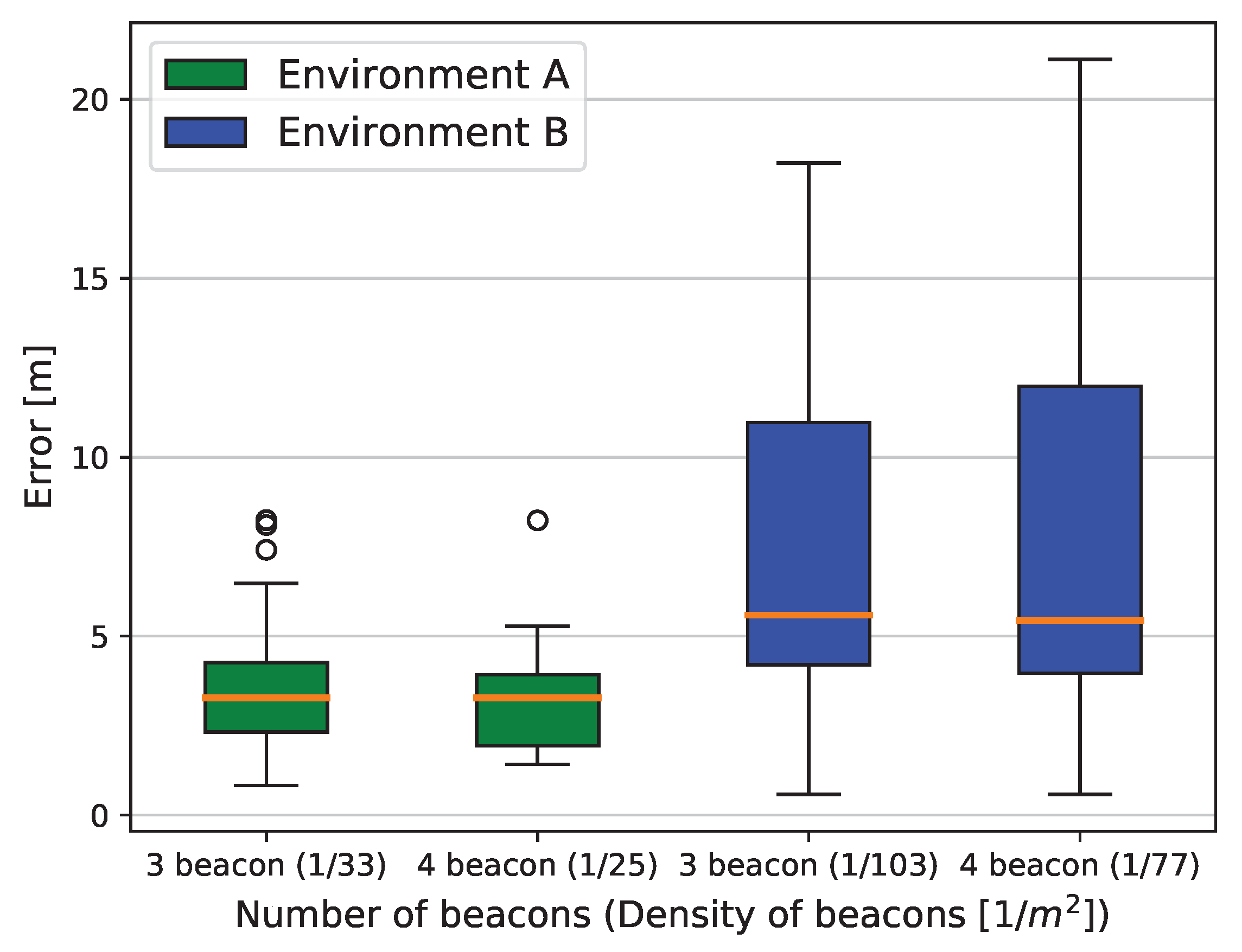
The error box plots for the trilateration algorithm, computed on all test points are reported in Figure 4 for both environments.

As shown in the graph, we performed measurements with either three or four beacons installed in each of the two environments, resulting in different beacons’ densities. In the case with four beacons, trilateration has been performed using the three strongest RSSI measurements at a given point.

As expected, the localization error is influenced by the density of beacons in the area, but the impact is minimal and the trends are not straightforward. In Environment A with four beacons covering an area of 25 m${}^2$ each, we obtain a median error of 3.3 m and an interquartile range (IQR) of 2.0 m. With only three beacons covering an area of 33 m${}^2$ each, the error median and IQR are practically unchanged, but the two extremes of the IQR are slightly shifted towards larger errors. For Environment B, the error clearly increases due to its wider area. For this environment, 4 beacons cover an area of 77 m${}^2$ each, obtaining a median error of 5.4 m and a IQR of 8.0 m. As for Environment A, when using only three beacons (each covering an area of 103 m${}^2$), the error median is practically identical, and surprisingly the IQR decreases to 6.7 m. However, the difference is not so significant, so also in this case the two results can be considered substantially equivalent.

Such large errors are clearly unacceptable for most indoor localization tasks, and clearly show the limits of simple RSSI-based distance algorithms. In fact, the median errors obtained with trilateration are significantly larger than the minimum half-distance between beacons (reported in Section 4.1), showing that this method does not reduce the error compared to a simple proximity-based localization. This is probably due to the fact that RSSI measurement precision is strongly affected by external noise sources, shadowing effects and multi-paths, which are particularly relevant in industrial environments. The fact that the RSSI is measured with a random device orientation also worsens the results.

Moreover, the results in Figure 4 show that increasing the density of beacons does not yield significant improvements to the localization accuracy. Of course, if these experiments were to be extended to a much higher number of beacons (e.g., >10), trilateration could indeed perform better. However, having such a high density of BLE devices would be unlikely in an industrial context, which is characterized by large environments and where the positioning of beacons is not always easy due to the obstructions caused by industrial machinery, etc. Moreover, the experiments of Section 4.3 show that fingerprint methods can significantly reduce the median error without resorting to a larger number of beacons, hence providing a lower cost solution.

For all these reasons, we conclude that the trilateration algorithm is not suitable for this type of environment and that a fingerprint method is indeed necessary.

4.3. Fingerprint Methods

Table 2. Median error and interquartile range (IQR) of fingerprint-based methods in Environment A and Environment B using four beacons and a fingerprint grid with one measurement every 0.5 m.

Method	Environment A	Environment B
SVM	median = 1.40 m	median = 3.52 m
	IQR = 0.82 m	IQR = 3.30 m
MLP	median = 1.82 m	median = 3.66 m
	IQR = 1.02 m	IQR = 2.85 m
k-NN	median = 1.33 m	median = 3.18 m
	IQR = 1.21 m	IQR = 3.37 m

reports the median error and the corresponding IQR for the three fingerprinting algorithms considered in this work. Errors are reported for both environments and refer to the case where 4 beacons are installed and the RFM measurements are collected every 0.5 m.

These results clearly show that fingerprinting helps in improving localization accuracy significantly, both in terms of median error and in terms of localization stability (i.e., IQR). SVM and k-NN show similar performance, with k-NN achieving the lowest median error in both environments. The MLP obtains the worst performance among the three tested algorithms. This is due to the low amount of training data available, which is typical for this application, where the amount of data are limited by the number of site RSSI characterization recordings. In general, the error increases for Environment B due to the lower density of beacons and to the presence of metal objects causing disturbances in the signals.

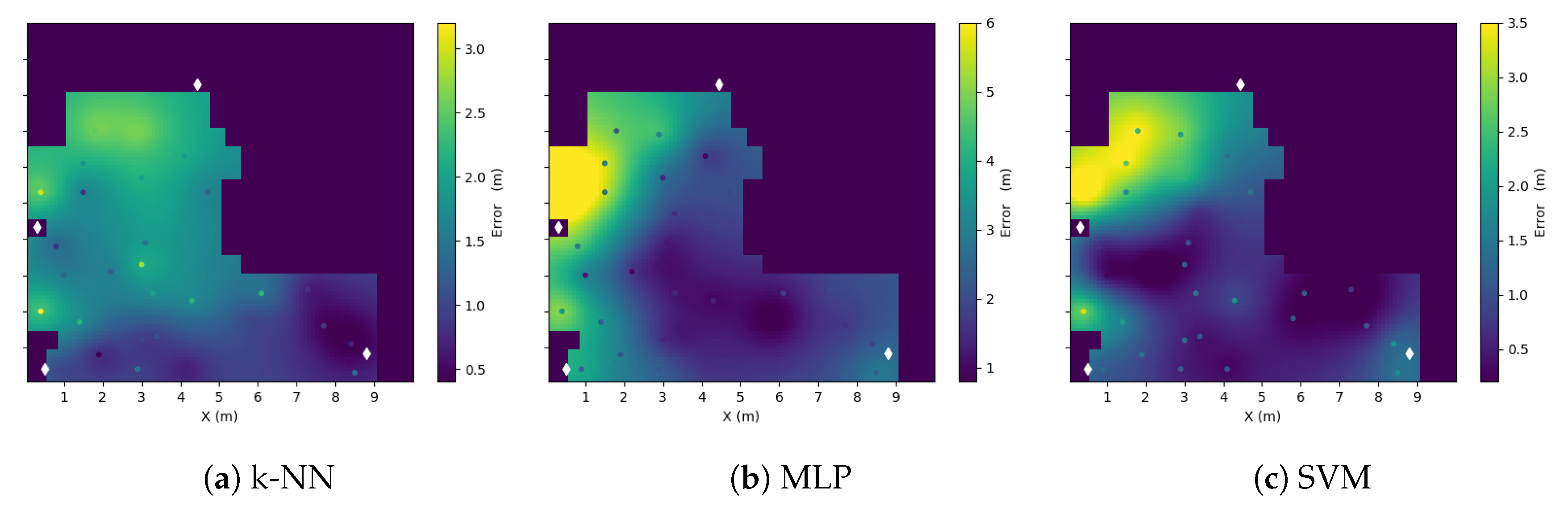
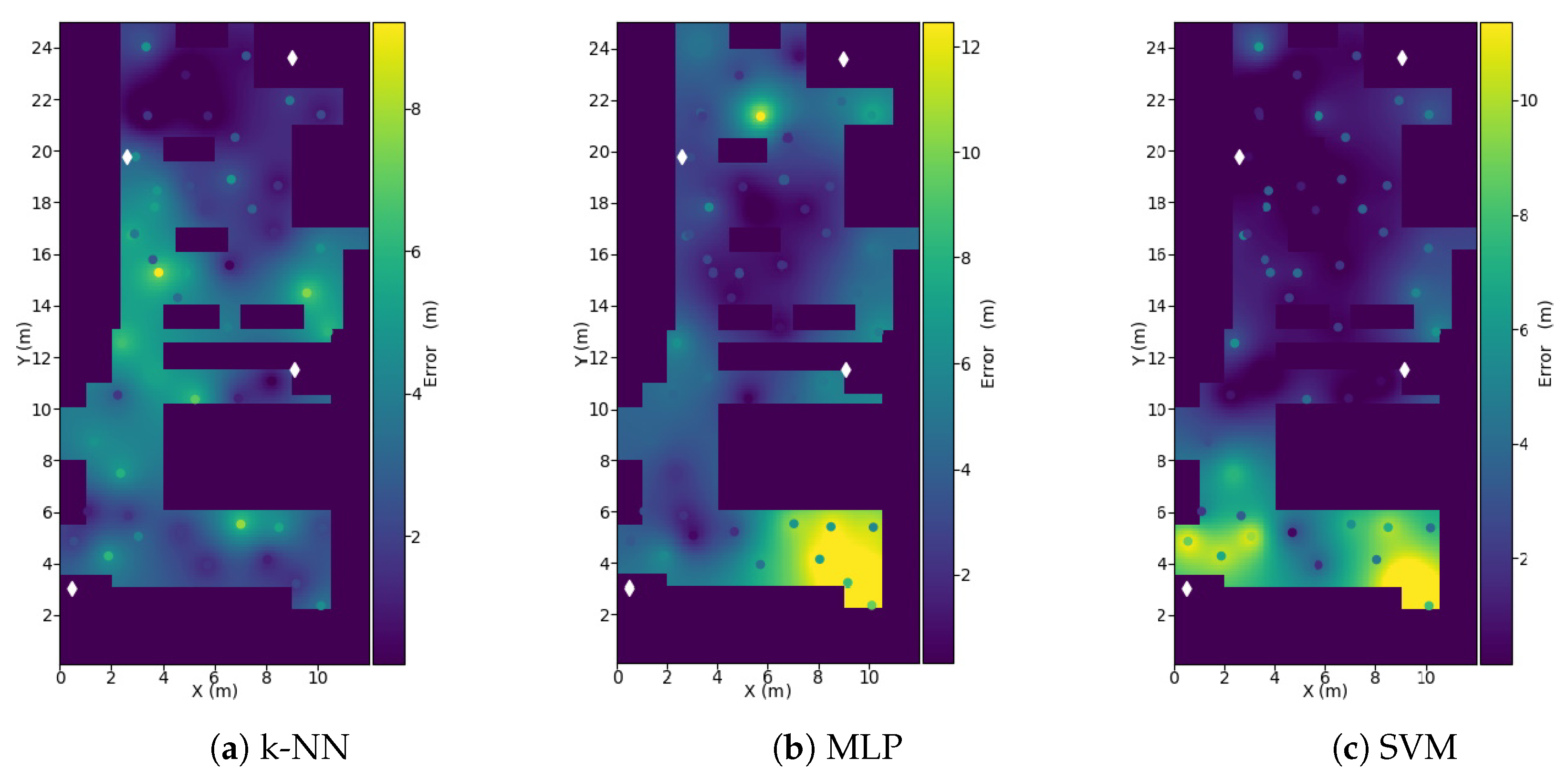
4.3.1. Error Maps

Figure 5 and Figure 6 show the map of the localization error of fingerprint algorithms for both environments. The positions of the four beacons are represented by white diamonds in the figures. The plots refer to the same experiment described in the previous Section (four beacons, one RFM measurement every 0.5 m).

Interestingly, Figure 5 shows that the area with largest error (>3 m) for Environment A is towards the left side of the room, where the wall is made of metal. Similarly, Figure 6 shows that SVM and MLP obtain a larger error (>10 m) in the bottom-right area, where there is a doorway made of metal and glass. k-NN seems to be less affected by the disturbances caused by these materials. In general, the map highlights that k-NN obtains the most stable estimate across the area of the two environments.

Table 3. Percentage of testing points lower than minimum half-distance between beacons.

Method	Environment A [%]	Environment B [%]
k-NN	$\approx 67$	$\approx 56$
MLP	$\approx 57$	$\approx 56$
SVM	$\approx 77$	$\approx 56$

reports the percentage of testing points whose error is lower than the minimum half-distance between beacons (reported in Section 4.1). As shown, for both environments, more than half of the testing points achieve a localization error that is smaller than the best result achievable with proximity-based localization, thus proving the effectiveness of fingerprint-based methods.

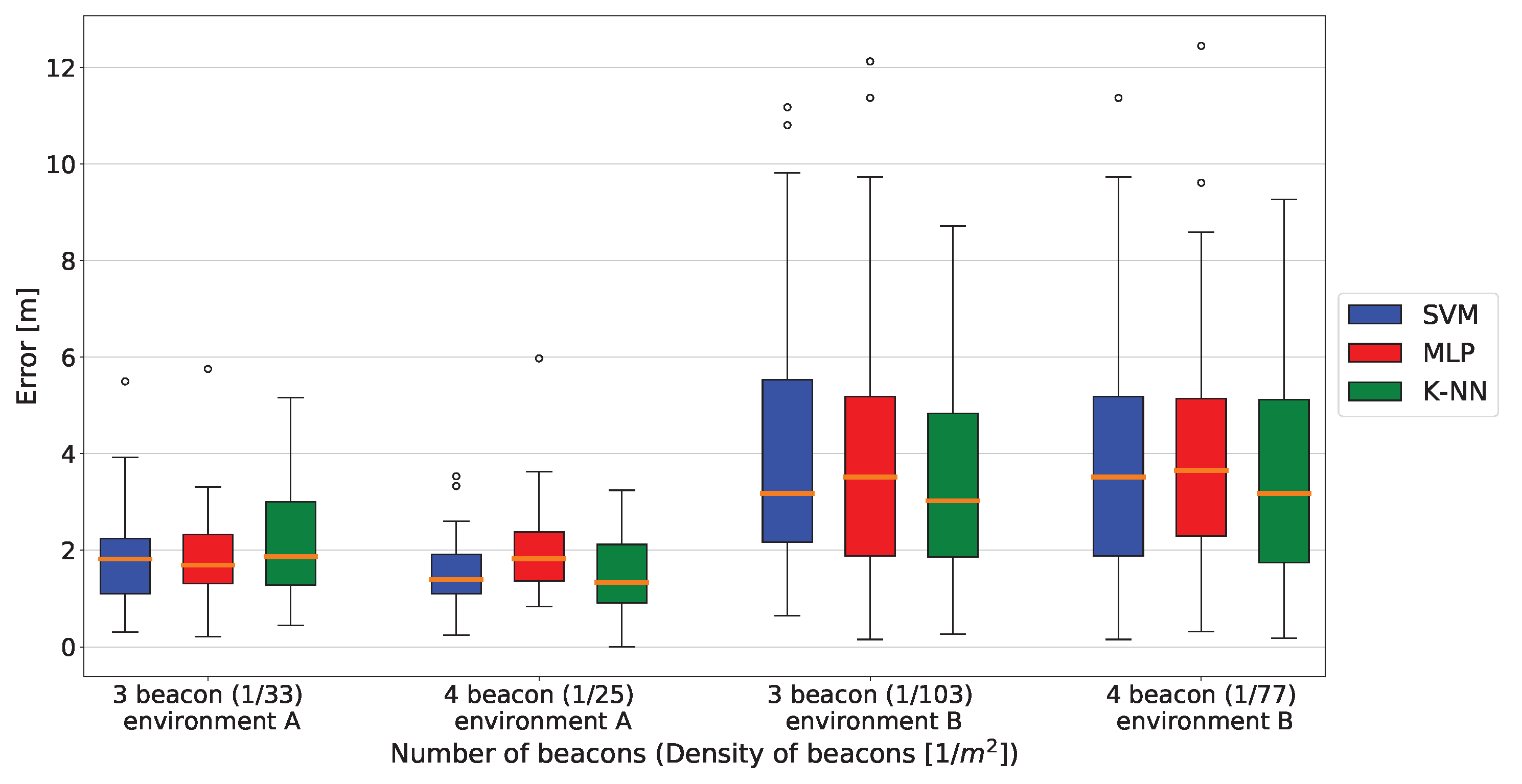
4.3.2. Impact of Beacons’ Density

Similarly to trilateration, we evaluated the impact of beacons density on the localization error in fingerprinting algorithms. As before, we tried decreasing the number of beacons in each environment from 4 to 3, leaving the density of the RFM grid unchanged (one measurement every 0.5 m). The results of this experiment are reported in Figure 7.

As shown, the error trends for SVM and k-NN are similar, and it is difficult to identify a clear winner. With either three or four beacons, SVM is slightly better than k-NN for Environment A, and vice versa for Environment B. For all three algorithms, the impact of having a larger number of beacons on the results is minimal. In general, the boxes identified by the IQR, as well as the “whiskers” of the box plots tend to shift towards lower errors when the number of beacons increases from three to four. However, the medians are often very similar and sometimes even increase. For instance, the median error of the SVM reduces by 0.4 m when going from three to four beacons in Environment A, but increases by 0.3 m in Environment B.

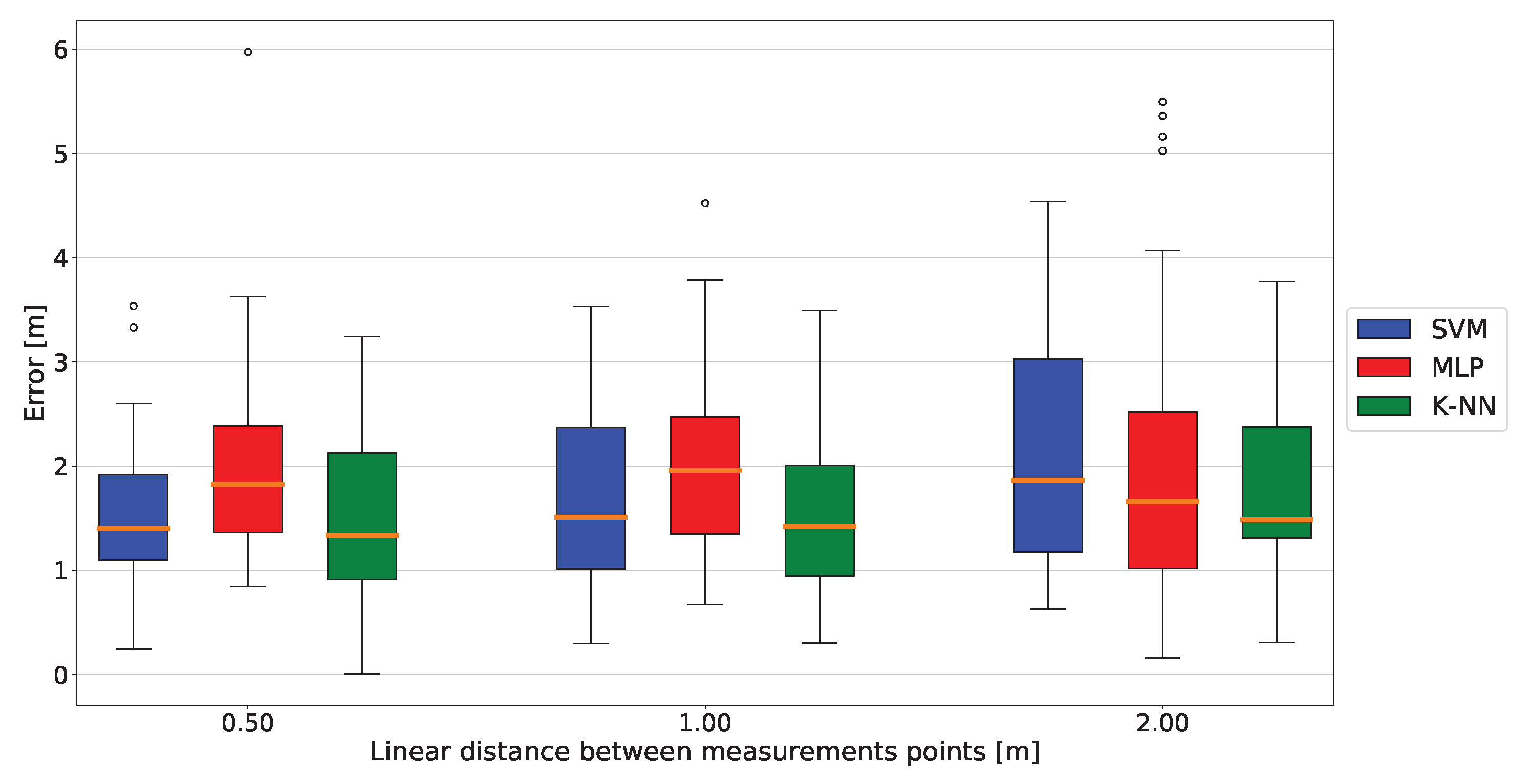
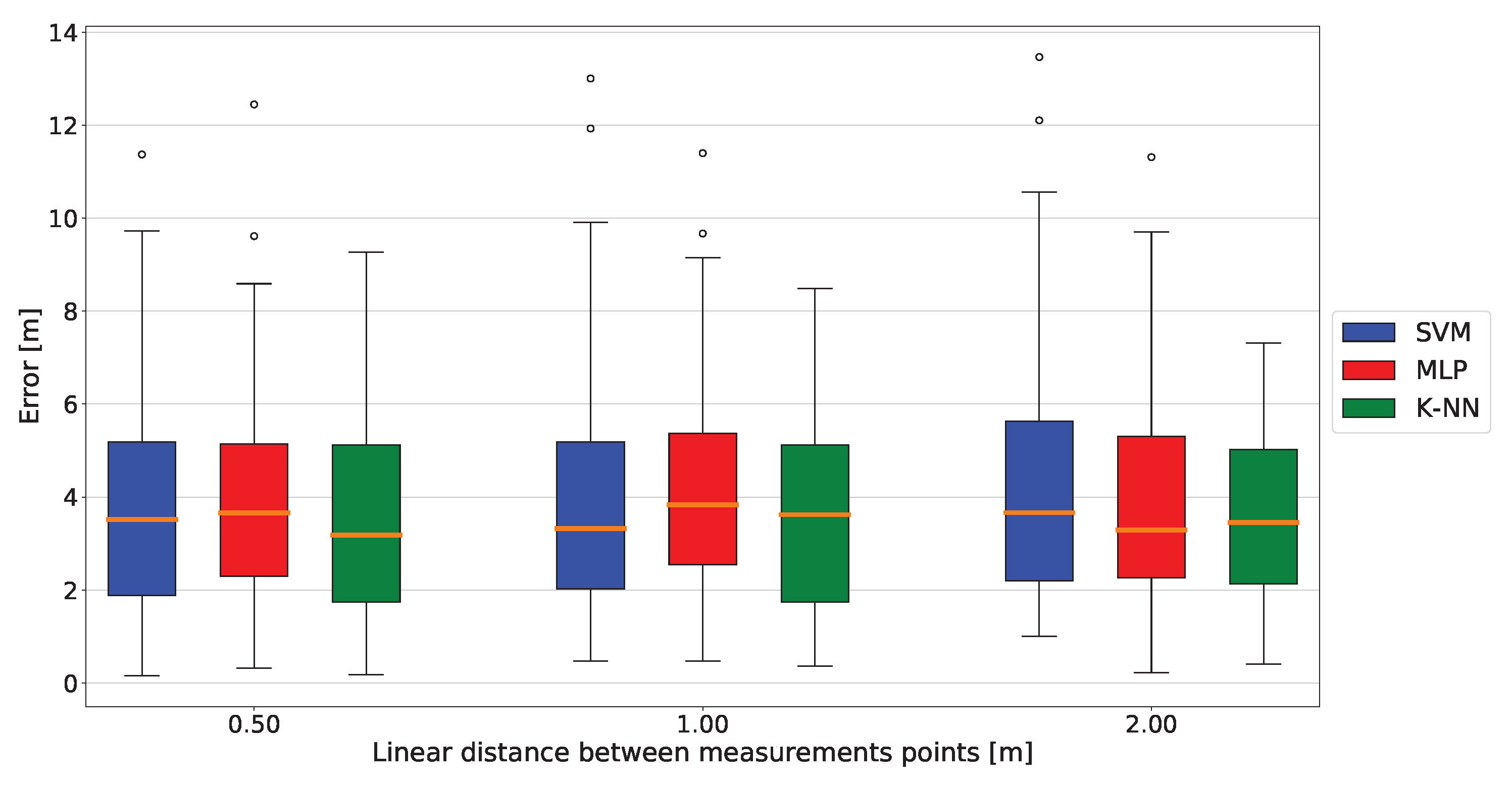
4.3.3. Impact of Fingerprint Grid Density

In fingerprint-based methods, the density of the grid map influences the performance of localization. To this purpose, we keep the number of beacons to four and we increase the number of RSSI measurements. In this section, we analyze the impact of this design parameter considering three fingerprint grids’ densities (one measurement every 0.5 m, 1 m, and 2 m). Figure 8 and Figure 9 show the results of this analysis for the two environments using four beacons.

Reducing the number of fingerprint points tends to cause a slight increase in the median error, in the values of the first and third quartiles, and in the length of the box plot whiskers. However, this is not always true and in general the impact is not dramatic, showing that even a quite “sparse” RFM is sufficient to obtain a decent localization accuracy. Once again, it is not easy to identify a clear winner among the three fingerprint algorithms. For example, in the smallest environment, SVM shows the most stable results with a dense grid (IQR = 0.8 m), but when the distance between the points increases, it is outperformed by k-NN (e.g., IQR = 1.1 m versus the 1.9 m of the SVM with one fingerprint point every 2 m).

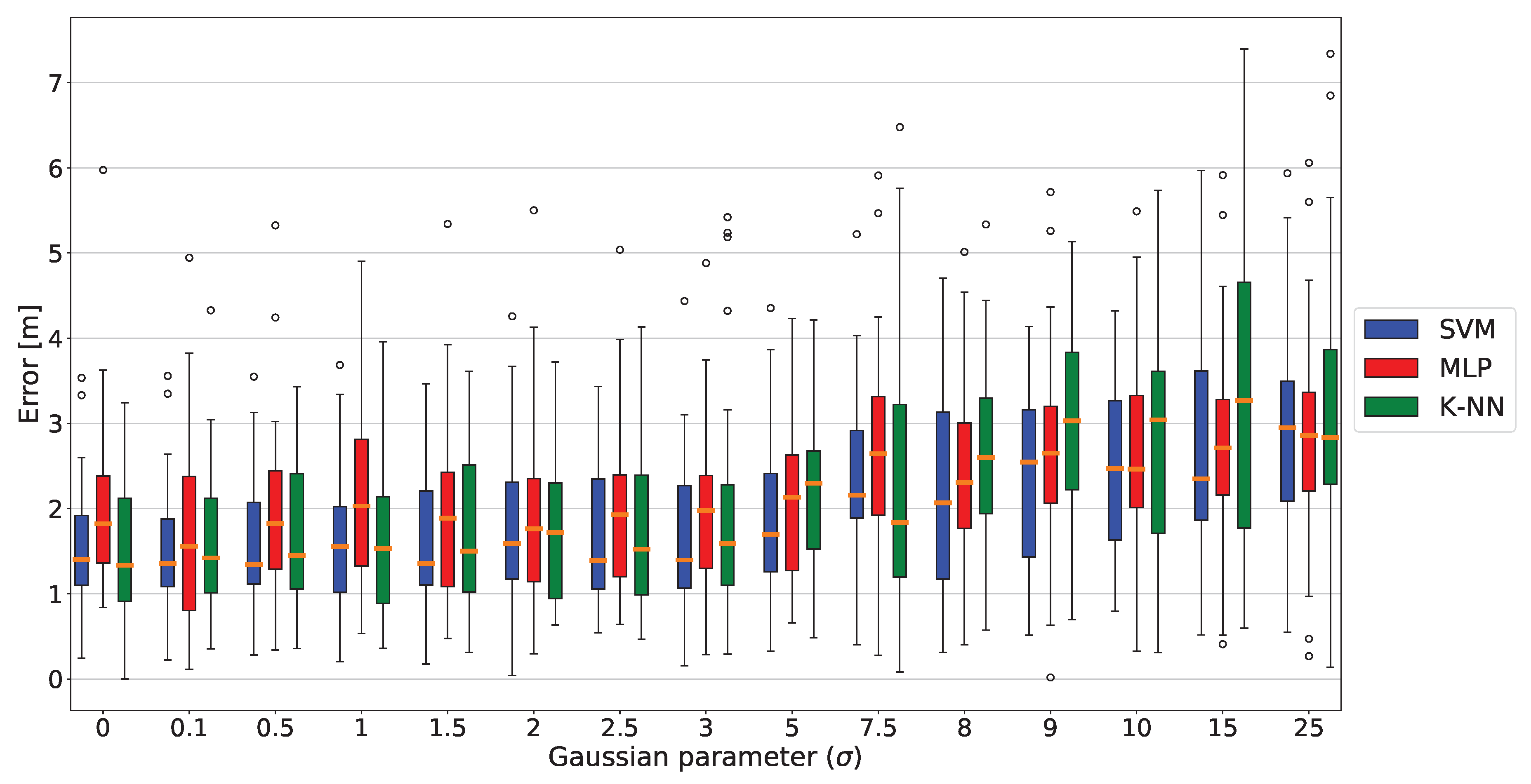
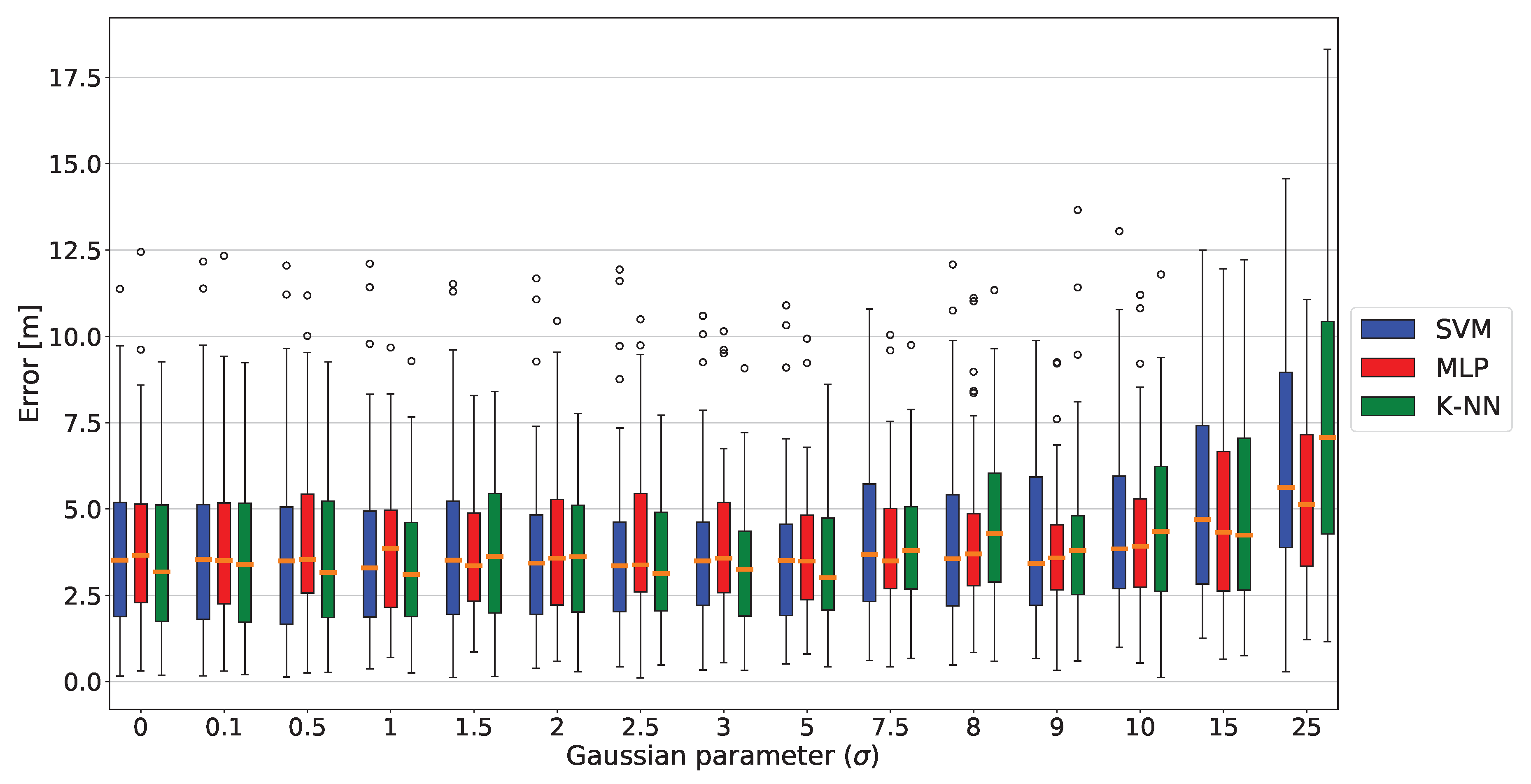
4.3.4. Impact of Environmental Perturbations

In an industrial environment, movements of large objects and machines may occur. Thus, a good localization algorithm should be resilient to environmental changes. This is clearly relevant especially for fingerprint-based algorithms, since when something changes within the environment the fingerprint data collected previously become obsolete and could lead to an incorrect positioning. Therefore, we test the effect of changes in the environment on the three fingerprint algorithms, first by simulation and then in the field.

The simulation is performed adding a zero mean Gaussian noise to the fingerprint RSSI values to mimic the scenario in which a variation in the environment makes them obsolete. Figure 10 and Figure 11 report the trends of the error box plots of the three algorithms as a function of the Gaussian standard deviation $\sigma$.

The three algorithms show a similar trend when Gaussian noise is introduced, and once again it is hard to state which algorithm performs better, since the differences in the box plots for a given value of $\sigma$ do not justify the choice of one algorithm over the other.

As a field experiment to test the influence of environmental perturbations, we introduce a large item (a 4 m × 4 m vehicle emulating industrial operations) in Environment A, then perform the localization without updating the RFM. The results obtained with the three algorithms in this scenario are reported in

Table 4. Error median and IQR for the three fingerprinting based algorithms in Environment A after adding a large object not present during the collection of the RFM.

Method	Environment A
SVM	median = 2.16 m
	IRQ = 1.02 m
MLP	median = 2.64 m
	IRQ = 1.39 m
k-NN	median = 1.83 m
	IRQ = 2.02 m

.

As expected, the median error in the test points increases for all three algorithms compared to the results of Table 2, but k-NN is slightly less affected by the perturbation than SVM and MLP, since its median error only increases by 0.5 m.

5. Conclusions

In this paper, we have presented a study that compares state-of-the-art indoor localization methods based on BLE in an industrial setting. Our results show that fingerprinting-based methods are sharply better than distance-based ones. This is motivated by the fact that the latter are affected by shadowing effects and reflections, which are particularly relevant in industrial environments, due to the presence of large moving metal objects.

Vice versa, the three considered fingerprint algorithms achieve very similar localization errors and show similar resilience to environmental variations and noise. Therefore, we argue that the selection of the best algorithm should be based on other aspects than sheer localization accuracy.

Even computational complexity considerations do not help the selection, as all three algorithms have a negligible time and memory complexity for the selected target device (the Raspberry Pi). Specifically, given the relatively small size of the training data (and consequently of the prediction models), we obtain that the inference execution time is <2 ms for all three algorithms, and the memory occupation is <40 MB.

Therefore, the final selection of an algorithm should be done based on training complexity and ease of adaptability, which directs the choice towards k-NN. In fact, this algorithm has a much simpler set of hyper-parameters (consisting solely of the number of neighbors k) compared to both SVM and MLP. This eases the deployment of a k-NN-based localization system in a new environment, as the only tests that need to be performed are those to identify the optimal value of k. Both MLP and SVM require a much more time-consuming parameter tuning for setting the number of layers, the number of neurons in each layer and the activation functions in the former case, or the basis function and values of $\gamma$, C and $ϵ$ in the latter. Moreover, k-NN does not require an actual training phase, which makes it more flexible for online adaptation. Specifically, whenever new or updated fingerprinting measurements become available, it is sufficient to update the database of reference points used by k-NN in order to obtain an updated location estimate. In contrast, such kind of update would require re-training in the case of SVM and MLP.

Therefore, we conclude that k-NN is the most suitable algorithm for industrial scenarios.