On Car-Sharing Usage Prediction with Open Socio-Demographic Data
by
 , , ,
, , ,
Michele Cocca
1,* ,
,
Douglas Teixeira
2,
Luca Vassio
1,
Marco Mellia
1,
Jussara M. Almeida
2 and
Ana Paula Couto da Silva
2 1
Department of Electronics and Telecommunications, Politecnico di Torino, 10129 Torino TO, Italy
2
Departamento de Ciência da Computação, Universidade Federal de Minas Gerais, Belo Horizonte 31270-901, Brazil
*
Author to whom correspondence should be addressed.
Electronics 2020, 9(1), 72; https://doi.org/10.3390/electronics9010072
Submission received: 12 November 2019
/
Revised: 7 December 2019
/
Accepted: 24 December 2019
/
Published: 1 January 2020
(This article belongs to the Special Issue Big Data Analytics for Smart Cities)
Abstract
:Free-Floating Car-Sharing (FFCS) services are a flexible alternative to car ownership. These transportation services show highly dynamic usage both over different hours of the day, and across different city areas. In this work, we study the problem of predicting FFCS demand patterns—a problem of great importance to the adequate provisioning of the service. We tackle both the prediction of the demand (i) over time and (ii) over space. We rely on months of real FFCS rides in Vancouver, which constitute our ground truth. We enrich this data with detailed socio-demographic information obtained from large open-data repositories to predict usage patterns. Our aim is to offer a thorough comparison of several machine-learning algorithms in terms of accuracy and ease of training, and to assess the effectiveness of current state-of-the-art approaches to address the prediction problem. Our results show that it is possible to predict the future usage with relative errors down to 10%, while the spatial prediction can be estimated with relative errors of about 40%. Our study also uncovers the socio-demographic features that most strongly correlate with FFCS usage, providing interesting insights for providers interested in offering services in new regions.
1. Introduction
Transportation in urban areas is among the top challenges to improve people’s quality of life and to reduce pollution. Historically, private vehicles have been the preferred mode of transportation. Orthogonally, governments invest in public transportation systems to offer alternatives to reduce traffic and pollution. With the rise of the sharing economy, we are now witnessing a transition towards new forms of shared mobility, which have spurred the interest of both the research community and the private companies.
Car sharing is an evolution of the classic car rental model. Here, users can rent cars on demand for a short period, e.g., a 20-minute trip across town. In particular, Free-Floating Car Sharing (FFCS) services allow customers to rent and return the cars everywhere inside an operative area in a city. Customers book, unlock, and return the car by using an application on their smartphones. In the FFCS implementation, the provider bills the user only for the time spent driving, with simple minute-based fares which factors all costs. Car2Go (https://www.car2go.com/) is one of the FFCS services that currently operates in several cities around the world. Some studies demonstrate that a massive adoption of car-sharing service can improve mobility as well as reduce costs and pollution [1,2,3].
To properly design and manage a FFCS service, a provider needs to know the demand for cars over different periods of the day, and over the different areas of the city. The prediction of FFCS demand patterns is thus fundamental for an adequate provisioning of the service. Armed with good predictions, the provider can better plan long-term system management, e.g., whether to extend the operative area to those neighborhoods with expected customer growth. Similarly, it can implement short-term dynamic relocation policies to better meet the demand in the next hours [4,5,6].
In this work we investigate the prediction of the usage dynamics of a real FFCS service. We aim at assessing how state-of-the-art machine-learning algorithms can help FFCS providers and policy makers in predicting the demand, both over time and across different spatial regions. More specifically, we leverage a dataset of real rides from cities where Car2Go is offering its FFCS service. We consider as a case study the city of Vancouver, Canada, the city with the highest demand for cars in our dataset. We rely on more than 1 million rentals covering 9 months in 2017 [7]. We augment the dataset by exploiting a rich and heterogeneous open dataset, namely the 2016 Vancouver Municipality census (https://opendata.vancouver.ca/pages/home/). This second dataset comprises more than 800 features, which detail very diverse information about shops in each neighborhood, weather conditions, residents, rate of emergency calls throughout the day, etc. Our goal is to first assess to which extent it is possible to predict the FFCS demand over time and space, and second, which of the features have a higher prediction power.
Our work focuses on two scenarios. In the first scenario, we investigate how to predict the demand for cars in the future considering past usage. This is fundamental for managing the FFCS fleet both in the short term (e.g., implementing relocation policies during service peak time), and in the long term (e.g., to properly match the fleet size to the future system growth). To this end, we analyse machine-learning algorithms that are considered state of the art, from simple Linear Regression and traditional Seasonal Auto Regressive Integrated Moving Average (SARIMA) models, to Random Forests Regression (RFR), Support Vector Regression (SVR) and latest approaches based on Long Short-Term Memory Neural Network (NN) [8,9]. With the increasing complexity of these models, we aim at assessing not only how they perform in our target prediction task, but also to which extent one would need to embrace a complex model (such as NNs are) or rather simpler and more informative models (like linear regression and RFR are).
In the second scenario, we correlate socio-demographic indicators with FFCS demand. We predict the demand of cars in a neighborhood without past data, using only socio-demographic data. This problem is often referred to as a green field or cold start approach. In this case, the operator is interested in knowing what the expected system usage in a new neighborhood is (or even a new city) based only on socio-demographic data. We map the FFCS demand to Vancouver neighborhoods, and associate them to the socio-demographic data coming from the official Vancouver census. We then use machine-learning techniques to highlight the relationship between demographics and customers’ mobility. We aim at answering the following research questions: (i) Using modern machine-learning methodologies, and armed with a rich socio-demographic data, would one be able to predict the temporal mobility patterns in a city? And (ii) which would be the most important socio-demographic data to use for this task?
Through a series of experiments, we show that the temporal prediction of rentals can be solved with errors as low as 10%. Interestingly, Random Forest Regression turns out to perform stably better than the other models, including Neural Networks, for this task. When considering the mobility prediction using only socio-demographic data, we obtain errors in the 40–50% range. While this performance may not be accurate enough for a precise planning, this prediction still would be useful for operators willing to decide, e.g., to which new areas of the city to extend their service. Interestingly, our models allow us also to observe what features are the most useful for the prediction problem, precious information for providers and regulators that wish understand FFCS systems—to decide, for instance, in which new cities to start a service (green field problem). Our work suggests, for example, that the density of people commuting by walk and the number of emergency calls in a neighborhood are important factors for predicting the number of rentals that will start there. We note that emergency calls are used as a proxy for human activity, i.e., the more human activity the larger the number of emergency calls. Given this assumption, we can leverage the information about the volume of emergency calls to improve prediction at different periods of the day. As for the temporal prediction, knowing the weather conditions in the near future would improve prediction too.
After overviewing the related work in Section 2, we describe the data collection methodology we adopt in Section 3. Section 4 provides a characterization of the datasets, while Section 5 and Section 6 provide details about the methodologies and results for the temporal and spatial prediction, respectively. Finally, Section 7 summarizes our findings.
2. Related Work
With the ease of collecting data and the ability to build and train off-the-shelf machine-learning solutions, researchers have started applying data driven approaches in the context of transportation. Previous work [10] addressed traffic modeling and prediction with real traffic data, and proposes strategies to improve congestion prediction using Kalman filters, showing how traffic is stationary in time. Other studies [11] proposed new approaches based on a multivariate extension of non-parametric regression to predict traffic patterns, with the goal of counteracting traffic congestion. While similar in spirit, our work focuses on FFCS services explicitly, and uses a much richer dataset as well as more advanced machine-learning algorithms.
Focusing on car sharing, early work focused on estimating demand using activity-based micro-simulation to model how agents move around in a city [12]. Later, as data from operative car-sharing platforms became available, researchers started using real data to analyze mobility demand. For instance, previous work [2,13] proposed a demand model to forecast the modal split of the urban transport demand. Similarly, other studies [3] investigated the Mobility-as-a-Service market, where FFCS is one of the implementations, and pointed out how FFCS supply can push the users to avoid purchasing a new car, which would lead to a reduction of emission. Yet, none of these prior studies focused on car-sharing demand prediction.
Along the same lines, other studies [14] made a large survey covering a Swiss station-based car-sharing service. The results confirmed that FFCS is preferred as a fast alternative to public transportation and the subscription depends on the car-sharing implementation (business model). Previous work [4] also proposed a simple binary logistic model for predicting car-sharing subscribers in Switzerland, considering the relationship between potential membership and service availability. This relationship was then used to identify areas with unmet demand, i.e., areas where new car-sharing stations could be placed.
Other studies [15,16] conducted a detailed characterization of a car-sharing system in Munich and Berlin. As with our work, they identified features correlated with the demand for shared cars in the target cities. However, our work differs from their in the sense that we here analyze a much larger set of features, including demographics and economic data, and consider multiple prediction models. We focus on demand prediction, facing both time and space dimensions, and provide a thorough comparison and guidelines for future directions.
In our previous work [17], we analyzed in depth the usage of different car-sharing systems in Vancouver. Based on this data, we developed a model of FFCS usage and built a simulator to design new systems based on electric vehicles [5]. In particular, we tackled the charging station placement problem, showing that the optimal placement requires few stations to satisfy charging requests in different cities [6].
To the best of our knowledge, we are the first to face the demand prediction problem in Free-Floating Car-Sharing Systems tackling both the temporal and spatial prediction with a real-world heterogeneous dataset. The demand prediction problem (or its variations) has been tackled in other domains [18,19], but we here focus on multiple prediction tasks (long-term, short-term) across different aspects (temporal and spatial) on the car-sharing domain.
Furthermore, while previous work [20] focused on the temporal prediction of car-sharing demand in a very short-term basis (demand prediction in the next few minutes), in this work we focus on the problem at different time scales. We also compare several prediction strategies and analyze how the temporal prediction problem relates to the spatial prediction one. Moreover, we are the first to use a very heterogeneous dataset including dozens of features to tackle the prediction problems. This allows us to provide insights on which of those features are the most important ones to solve our prediction problems as well as to have a broader perspective on the challenges involved in car-sharing prediction.
3. Data Gathering Methodology
3.1. FFCS Data Collection
We collect data from Car2Go, a popular FFCS system that offers its services in more than 25 cities and 3.6 million customers in 2019. Briefly, Car2Go works as follows. The system knows the position of all cars (available or not) in the fleet. A customer looks for and reserves an available car by using a smartphone application, after which he or she can rent and drive the car. At the end of the ride, the customer parks and returns the car by notifying the FFCS system via the smartphone application. The system records the new position of the car, and makes it available for other customers.
Car2go allows developers to interact with their services through a public Application Programming Interface (API) (The use of the Car2Go API (https://www.car2go.com/api/tou.htm) is subject to approval by Car2Go. We got the approval in September 2016 and continued to collect data until January 2018). With this API, we can retrieve the current position of available cars in a given city. Each car is identified by its plate, and it is possible to identify rentals by simply performing periodic queries. In our previous work, we developed a system for collecting data from Car2Go’s API [7]. This same system, called Urban Mobility Analysis Platform (UMAP) is used in this work. It allows us to systematically collect precise data about car rentals in all cities where Car2Go offers its service. More specifically, UMAP queries the Car2Go API every minute to get the currently available cars. It then rebuilds the history of rentals of each car, identifying bookings and parkings. A booking is the time period in which a car is booked by a customer (or in maintenance). Conversely, a parking is the time period during which a car has been available for a ride to users.
Since customers can reserve a car and then cancel the reservation afterwards without actually renting it, we consider a rental a booking with (i) distance between starting and final locations greater than 500 m; (ii) travel duration shorter than 1 h. In a nutshell, we discard those bookings which where not converted into rentals (i.e., when the user reserved the car without actually driving it), and those rentals where the car disappears for long periods (i.e., possibly due to maintenance). We refer the reader to previous work [7] for a detailed analysis of these implementation decisions.
Here we focus on Car2Go rentals recorded in Vancouver for 10 months during 2017. We chose the city of Vancouver as a case study for two reasons. First, among the cities where Car2Go offers its service Vancouver is the city the highest number of rentals per day. Second, because of the amount of open data made available by the Vancouver municipality. In total, we collect more than 1 million rentals that we use as ground truth to train and test machine-learning algorithms to predict service demand across time and space.
3.2. Socio-Demographic, Weather and Other Open Data
In addition to information about rentals in the city of Vancouver, we also use socio-demographic data as input to car usage prediction algorithms. Specifically, we consider the Vancouver census open data (https://opendata.vancouver.ca/pages/home/), which divides the city in 22 official neighborhoods. Our work uses this same spatial division. For each neighborhood, the census dataset provides detailed socio-demographic information such as number of residents in a given age range, their income, household compositions, and commuting habits. The census also reports information about services that are in the neighborhoods, e.g., shops, bus stops, and parking places. In total, the census presents more than 800 socio-demographic and other spatial features. Among those, we manually selected 83 features that might be related to human mobility (the complete list of features is available at https://opendata.vancouver.ca/pages/census-local-area-profiles-2016-attributes/). In addition, we also consider (i) the distance to downtown—computed as the distance from the neighborhood to the downtown neighborhood (considered to be the central area; We use the neighborhoods central points for distance computation). (ii) an indicator of human activity, measured by the number of emergency calls per time bin (obtained from the Vancouver census); and (iii) the hourly weather for Vancouver—as directly available from the OpenWeather project (https://openweathermap.org/history-bulk). For each of the 22 neighborhoods, we normalize each numerical feature by the area of the neighborhood. Our goal is to include a super-set of features possibly correlated with human mobility and thus car rental prediction, to provide the machine-learning algorithms with an input dataset as rich and diverse as possible to learn from.
4. Dataset Overview
We first provide an overview of the data at our disposal offering insights into the diversity and heterogeneity present both in the temporal and spatial FFCS usage patterns as well as in the socio-demographic data.
4.1. FFCS Temporal Characterization
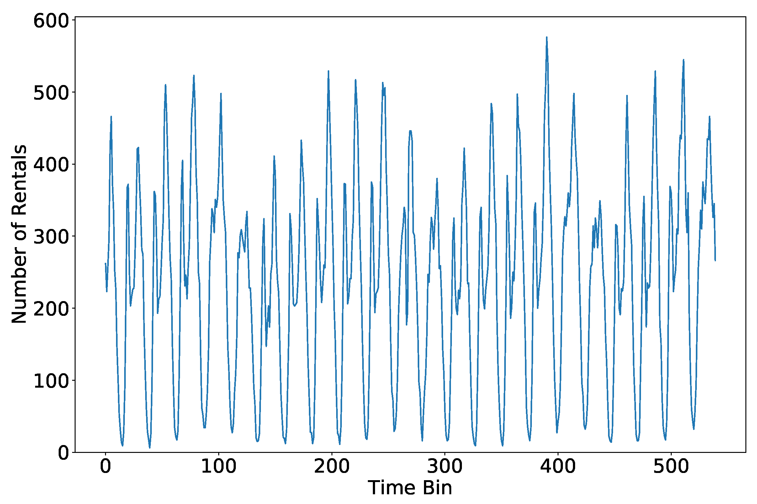
We start by showing the temporal evolution of rentals over time. Figure 1 shows the total number of starting rentals per hour in the whole city during part of September 2017. Even if we can spot some periodicity, there is a lot of variability that makes the prediction problem not straightforward. For our analyses, from now on we aggregate rentals both in time and in space. Specifically, given a neighborhood we consider the fraction of rentals starting and ending there. We aggregate the time series of rentals into 7 time bins per each day, namely from midnight to 6am (night period), and then every 3 h. This time granularity is typically used for system design and management [16]. The rationale is to provide the FFCS company that actionable information on the demand for cars, e.g., to schedule car maintenance or implement relocation policies. A one-hour period is often too short for the company to be able to respond to changes in demand.
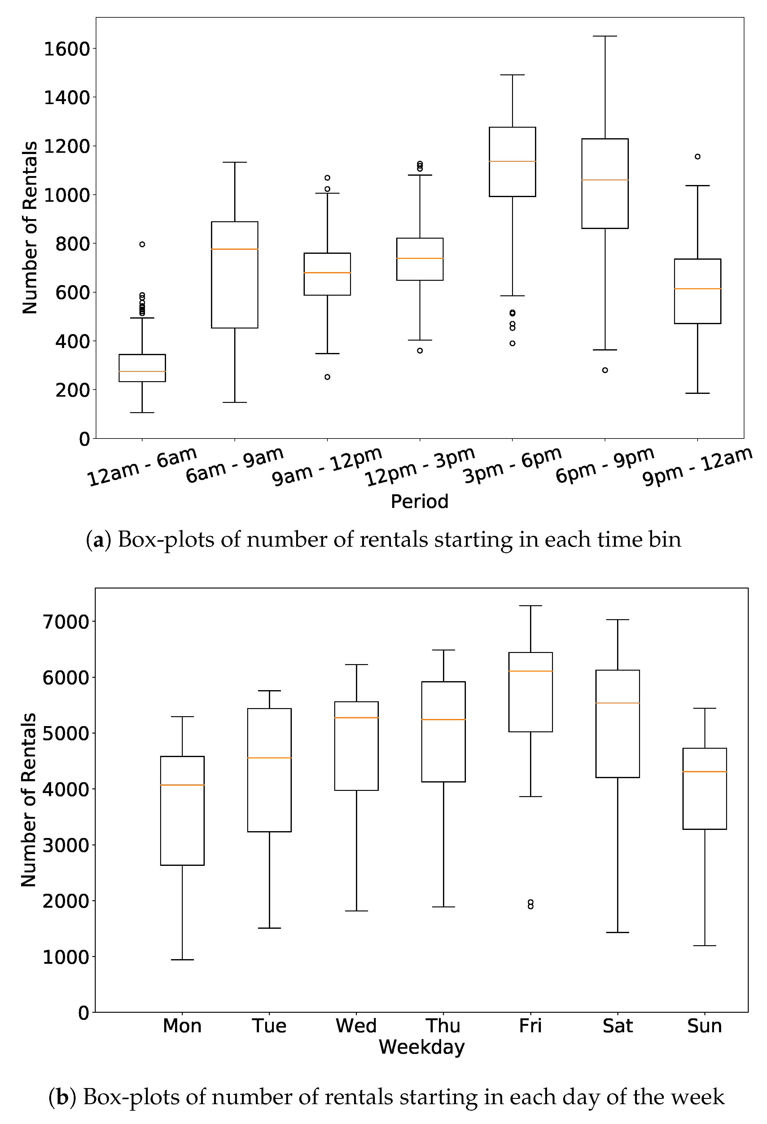
To give more details about the variability of the data, Figure 2a shows box-plots of the numbers of rentals starting in each time bin. Each box-plot represents the quartiles of the distribution, with outliers shown as points (We consider as outliers those points that are outside the mean ±2.698 times the standard deviation range). The series shows large variability, with peaks during early mornings (6–9 am) and afternoon (3–6 pm and 6–9 pm), and with low values during nighttime (12–6 am). Figure 2b shows box-plots of the total number of rentals grouped per day of the week. The number of rentals peaks on Fridays, with significantly lower values registered on Sundays and Mondays. Again, we observe a quite size-able variability over the days, as observed by in the size of the box-plots. Such variability hints at the fact that prediction models must be able to deal with size able temporal variations in the demand for cars.
4.2. FFCS Spatial Characterization
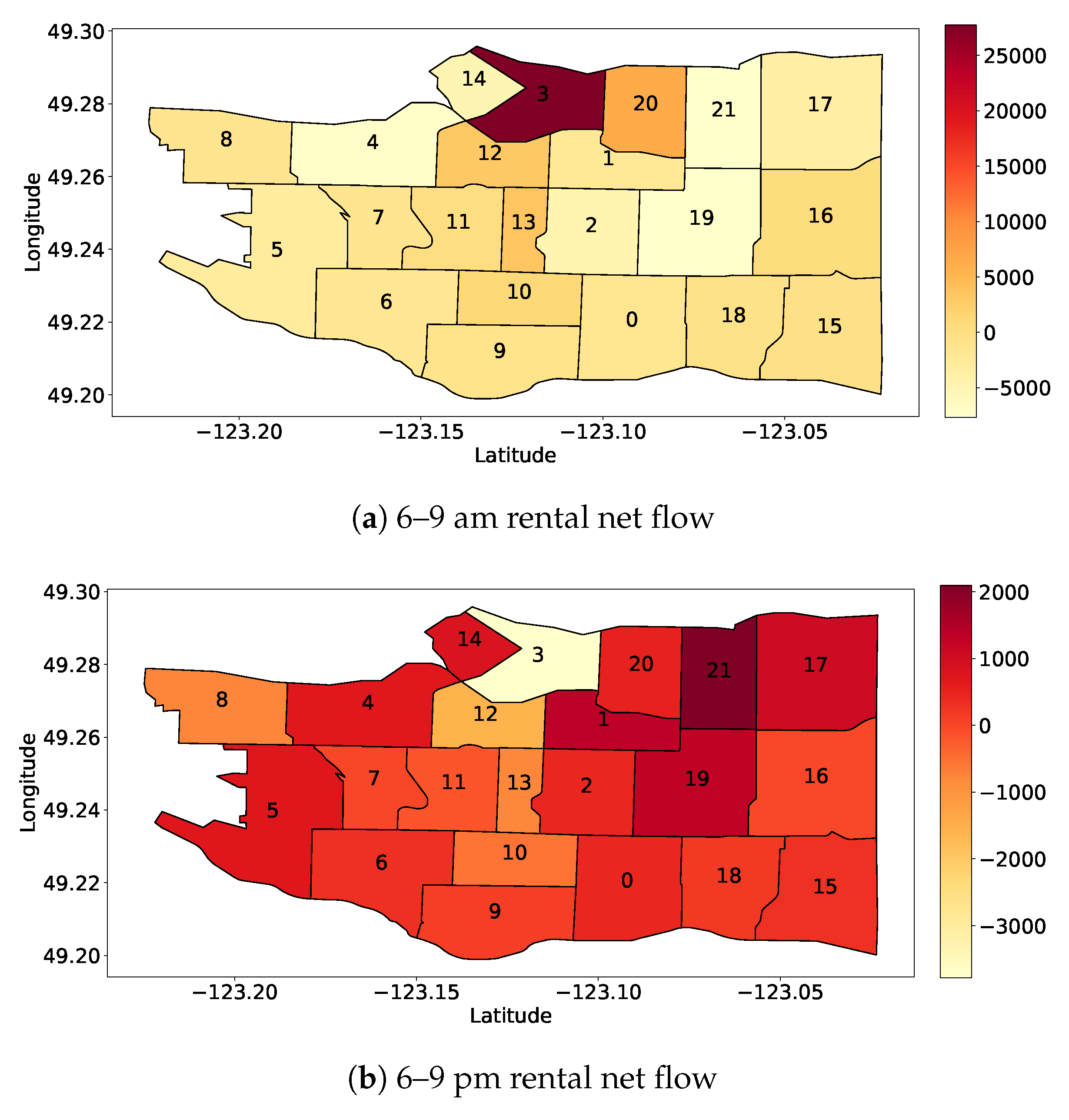
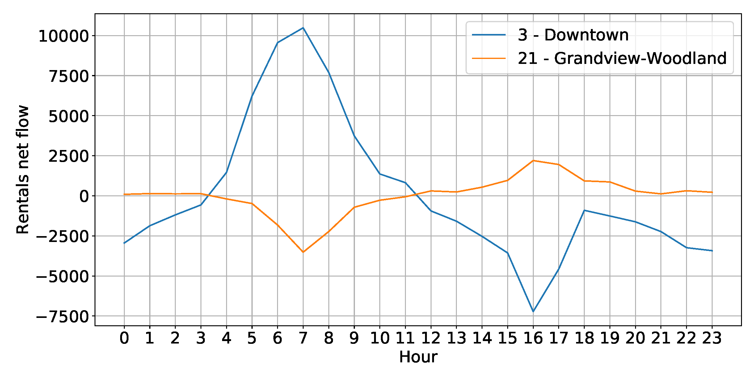
We now take a closer look into how these figures vary across different areas of the city. Rather than providing a complete characterization of the origin/destination matrix (which is outside the scope of this work), we here focus on particular examples to showcase the spatial variability in the demand for cars. We focus on the morning and afternoon peak time bins (6–9 am and 6–9 pm). For each neighborhood we compute the net flow, defined as the difference between the number of rentals starting from that neighborhood and the number of rentals arriving at that neighborhood during the specified time period. We consider the cumulative net flow in September 2017. Figure 3b depicts the results with a heat map. Darker red neighborhoods mean that arrivals exceed departures, i.e., the neighborhood is attracting vehicles. Conversely, lighter colors imply that more vehicles are departing from that neighborhood than arriving in it. Numbers identify different neighborhoods. The downtown business area (number 3) attracts a lot of rides in the morning period (Figure 3a), while the opposite pattern is seen during the afternoon period (Figure 3b). In general, we can assert that the FFCS demand is higher in the peak hours, and the cars flow towards downtown in the morning and towards residential areas in the afternoon. This is clearly visible in Figure 4 which reports the total net flow for two neighborhoods for each hour of the day, namely the downtown neighborhood (number 3), and the Grandview-Woodland (number 21) neighborhood, a residential area close to downtown.
4.3. Socio-Demographic and Weather Data Characterization
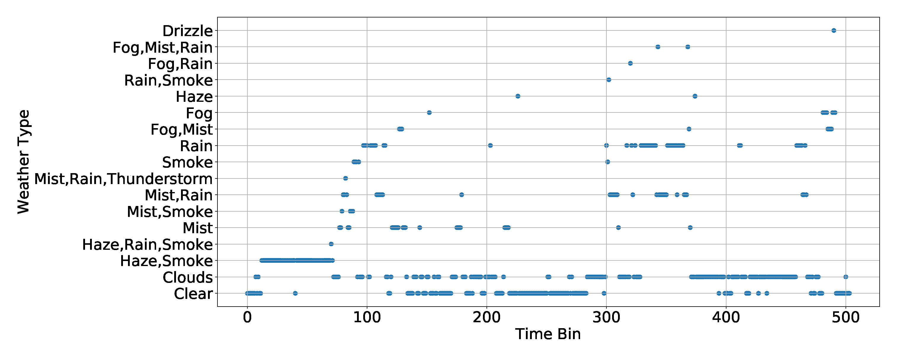
We now provide some examples of the socio-demographic and open data. Figure 5 reports the weather condition during the month of September 2017. It being a categorical variable, we assign to each weather condition a different value on the y-axis. As expected, the weather conditions change over time quite frequently. Moreover, no visible correlation is found when comparing the weather conditions with the number of rentals in Figure 1.
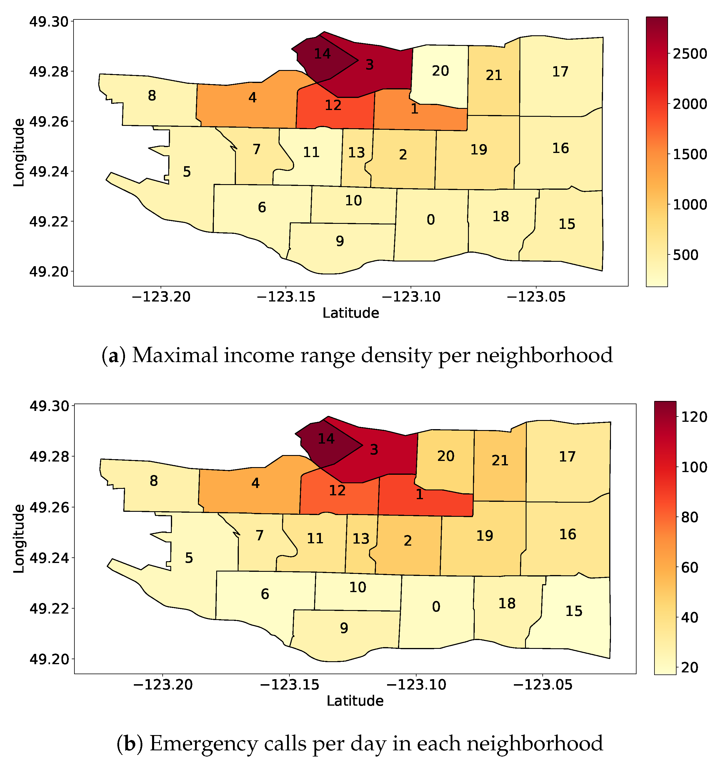
Similarly, Figure 6a,b show the number of high-income households and the number of emergency calls per day for each neighborhood, respectively. Also in this case, it is hard to see any clear correlation with the net flow per neighborhood reported in Figure 3b. The scenario is similar considering other socio-demographic features.
Despite the non-linear correlations between the socio-demographic data and rentals, it is possible that the combination of multiple features helps the prediction of car rentals, as we will discuss in the next sections. This is exactly what the machine-learning algorithms aim at, i.e., building a model from data, leveraging correlation from multiple variables that, considered together, carry enough information to predict system usage. Thus, we let the machine-learning model decide if and how to factor different features in the prediction model.
5. Temporal Predictions of Rentals
In this section, we describe our task of predicting the number of rentals in the whole city at a given time in the future. Eventually, the same methodology could be applied for each neighborhood. This prediction can exploit historical data, i.e., given the time series of rentals in the past, predict the number of rentals in the future. If only the past time series are used, the problem falls in the univariate regression class, i.e., the prediction is based only on past data of the same target variable. Let be our target variable, i.e., the number of rentals at time t. In the case of prediction with historical data, we predict
as a function of the past data points of x itself. j is the horizon of the prediction.
If we also have other information, we can build a more generic model to consider the dependence to other variables. We want to predict
where are different variables—possibly other time series themselves (including x)—and g is the model that allows us to predict x at time . This problem is a multivariate regression problem, where multiple features are used to predict the target variable x.
Considering the time horizon of the prediction, we can formulate two versions of the problem: predict the long-term or short-term usage. In the first case, we build and train a single model using all data at our disposal to predict the system usage in the next months. In the short-term version, we target the prediction of the next time bin only, i.e., . In this second case, we build and update a new model at each time bin by adding the latest recorded number of rentals to the training set as soon as it becomes available.
Both predictions are important for the car-sharing provider. For instance, the long-term predictions are important to know if their fleet size is enough to keep up with the expected demand. The short-term is important to know when to take a car down for maintenance, or when and where cars should be eventually relocated to those neighborhoods where the demand is expected to increase shortly. While for long-term prediction we use the time series of the rentals and information about day of the week and hour of the day, for short prediction we can also use the near future weather condition information.
In this work, we consider discrete time, i.e., we split time into fixed size time intervals as defined in the aggregation step—see Section 4 for more details. We then build and train several machine-learning models to tackle each aforementioned problem. Our goal is to compare algorithms in terms of accuracy of the prediction and complexity of the model. At last, we are also interested in considering models that are interpretable, i.e., that allow us to understand which are the most important features that affect car-sharing usage in large cities. We evaluate all models considering three metrics: APE (absolute percentage error), MAPE (mean absolute percentage error), and RMSE (root mean square error) over the validation set. The APE is defined as
where V is the validation set, is the actual value of the data at moment and is the predicted value. The MAPE is then given by
and the RMSE is defined as
5.1. Prediction Models
We use off-the-shelf machine-learning models both for the long-term and short-term scenarios. We consider the following univariate models: a simple baseline (BL) approach, the auto-regressive moving average (ARIMA) and the seasonal auto-regressive moving average (SARIMA) algorithms. Univariate models do not account for the influence of other time-variant factors such as weather conditions, time of day, number of emergency calls, etc. To account for that, we also investigate the performance of linear regression, Random Forests Regression (RFR), Support Vector Regression (SVR), and long-term short-term memory neural networks (NN).
We add categorical features (the day of the week and weather, for instance) to these algorithms to improve on the univariate models. Following correct practices [21], we represent each categorical feature as many binary variables, one for each category. For example, when representing a given weather type, the corresponding binary variable will be set to while all the other weather-related variables to . We used the algorithms implementation in Python libraries scikit-learn (https://scikit-learn.org/) [22] and Keras (https://keras.io/). Our code for the analysis is publicly available at https://github.com/dougct/carsharing-prediction. For details about each model, we refer the reader to [9]. In our implementations, we start with the library’s default hyper-parameters and conduct a grid search to find a set of such parameters that worked well with our models. We report the range of the grid search along with the description of the models below.
Baseline. A simple approach to determine in a time bin is to take the average number of rentals in the same time bins in the available past days. We compare all our prediction models to this baseline.
ARIMA. ARIMA (auto-regressive integrated moving average) is widely used to predict time series data. ARIMA models are a combination of auto-regressive models with moving average models. The creation of an ARIMA model involves specifying three parameters . The d parameter measures how many times we must differentiate the data to obtain stationary data. After determining d, we use sample partial auto correlation function to get the value p. Finally, we determine the order q by looking at the sample auto correlation function of the differentiated data. For simplicity, we restrict our grid search to find the best parameters values to the range . The combination that gave us the best results is .
SARIMA. A SARIMA model incorporates the seasonality (periodicity) of the data into an ARIMA model, enhancing its predictive power. For instance, when modeling a time series, it is often the case that the data has a daily, weekly, or monthly periodicity. We used our previous ARIMA model with an additional explicit daily seasonal component ( as the number of time bins in a day in our case).
Linear Regression. We fit a linear model by finding the coefficients that multiply each feature.
SVR. In our experiments, we use a Support Vector Regression (SVR) model with the following combination of parameters, which produce the best results among the values we tested: , , and , with the RBF kernel. The values for the parameters , and were evaluated in the range , and for the C parameter we considered the range , using exponential steps. The value 1000 was chosen once it provided a reasonable balance between model performance and generality.
RFR. Random Forest Regression is an ensemble learning method that can be used for regression. The decision is based on the outcome of many decision trees, each of which is built with a random subset of the features. One advantage of random forests over linear regression is that the forest model can capture the non-linearity. Another advantage of RFR is that they are interpretable models, i.e., they offer a ranking of the most important features for the prediction problem. Here, we use 50 decision trees (Throughout the manuscript, interpretable refers to the fact that it is possible to understand the decision taken by the classification model. However, interpretability has not to be confused with explainability, which refers to the motivations of the decision. The latter is only possibly via domain knowledge). In this model, we use the default library parameters, but we evaluate the impact different numbers of trees, for which the results are shown in the next sections.
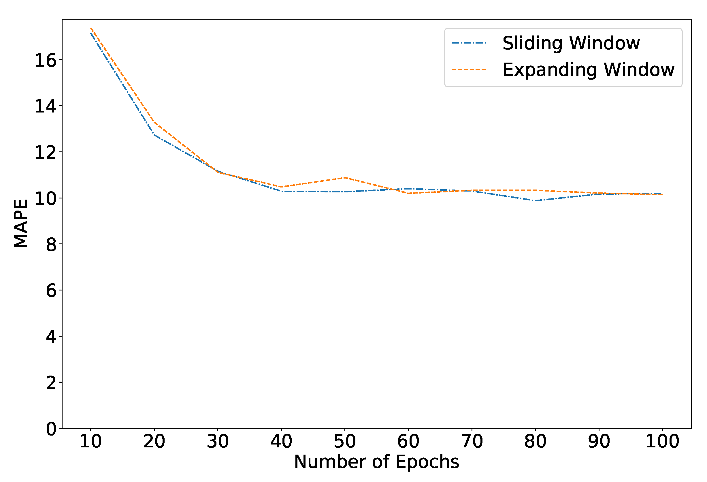
Neural Networks. We also consider a Long Short-Term Memory (LSTM) Neural Network model. LSTMs have a memory that helps capturing past trends in the data, which may favor our prediction task. We experiment with several different architectures. In particular, we test different configurations for the architecture: the number of neurons varies in the range for the first layer, and in the range for the second layer. Because of the nature of the task (regression and not classification), the number of neurons in the third layer is set to one. The best results are obtained with a three-layer architecture where the input layer has 64 neurons (one for each feature), the dense layer has 4 neurons, and the output layer has one neuron. In our experiments, to balance prediction accuracy and training time, the model is trained for 50 epochs. As we will see in Section 5.3, increasing the number of epochs to more than 50 has no significant effect (less than 1% reduction in the MAPE, on average) on performance.
5.2. Long-Term Predictions—Results
Here we predict the FFCS demand for cars in the future months given a model built on the previous months. We use in our experiments car-sharing usage data for the first nine months of 2017 in the city of Vancouver. Given the volume of rentals in the training period, we try to predict the number of rentals in the validation period. For that, we use a model that is trained once and then used to perform all the predictions in the validation period. Our training set consists of the volume of rentals for the first six months, and the validation data consists of volume of rentals for the next three months.
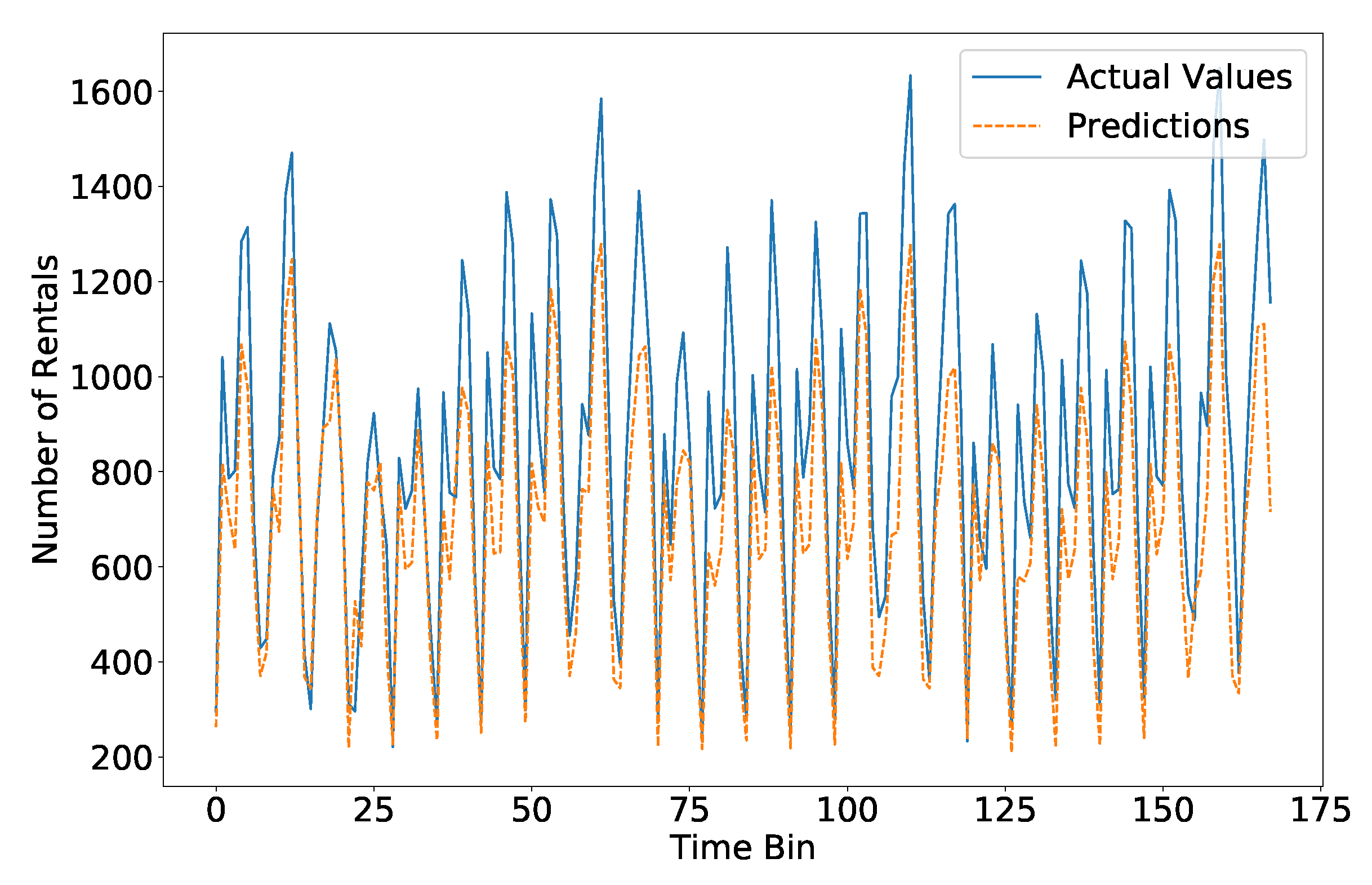
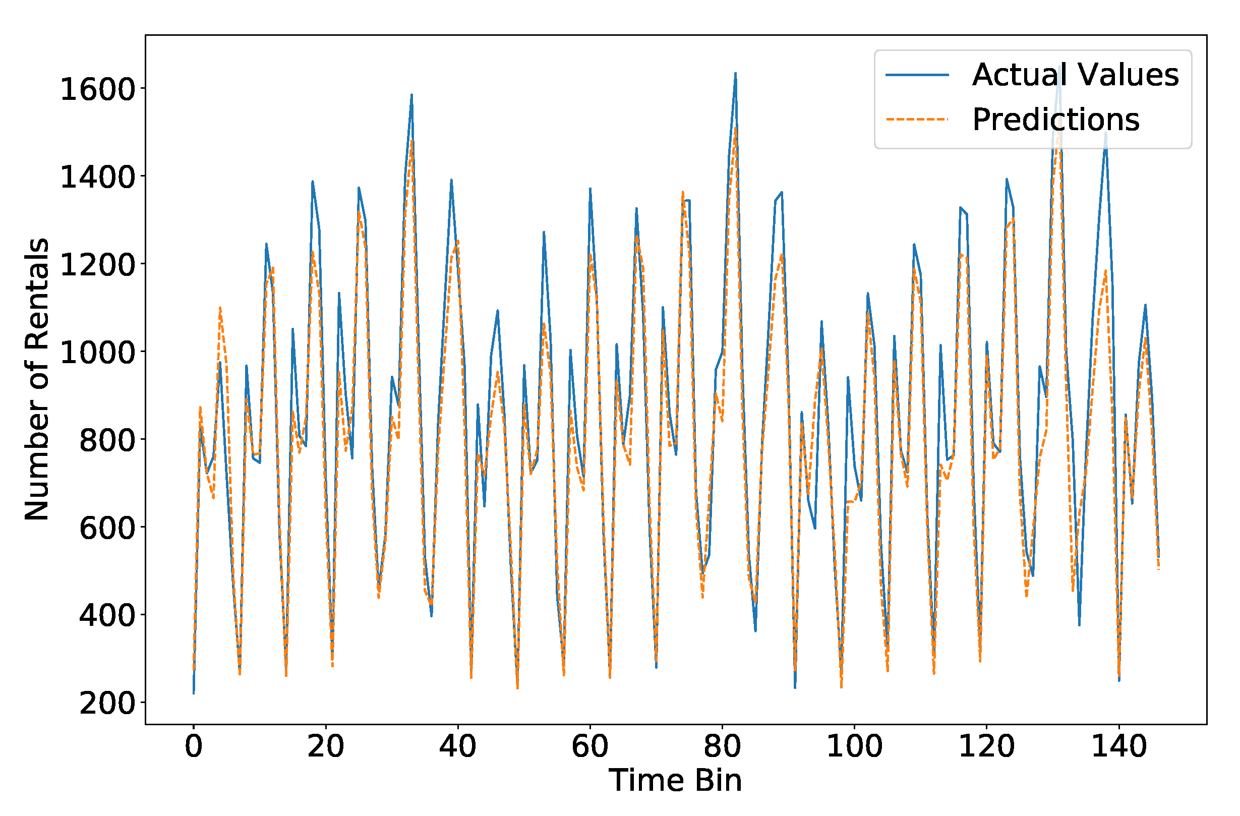
Table 1 shows the average mean absolute percentage error (MAPE), the standard deviation of the APE, and the RMSE for each of the prediction models. The models that rely only on the time series (ARIMA and SARIMA) can capture some patterns in the data, as their performance is considerably better than the baseline. However, the multivariate models perform better, with Random Forest Regression reaching the best performance. In Figure 7 we show the comparison between the actual values and the prediction in one month of the validation set using the Random Forest Regression model (orange dashed line). Overall, the model can predict quite well the daily and weekly periodicity of rentals, but in general it slightly underestimates the actual number of rentals. This could be due to the fact the training period refers to the first six months of the year, during which the average number of rentals is lower than during the validation period (Fall season).
5.3. Short-Term Predictions—Results
We now tackle the problem of predicting the demand of cars in a city in the next time bin. Differently from the long-term predictions we use adaptive models, i.e., the model is re-trained every time new data is made available, then we can add it to the training set. We here focus on the following prediction task: given the volume of rentals per time bin period for a specific number of past days and the weather conditions in those days, predict the number of rentals in the next time bin period.
We study this prediction task using two approaches: expanding window and sliding window. In the expanding window approach, after making the first prediction, we add the actual value to the training set, therefore increasing the amount of data available for training in the next step. To train our models, we first set aside 24 days of data for validation, and start with 28 days of training data. In the sliding window approach, after making the prediction we remove the oldest training data and add the actual value to the training set. Therefore, the training set size is always the same during the evaluation of the models. To train our models, we consider different sliding windows sizes (from 7 to 28 days), and validate on the same validation set of 24 days as with the expanding window.
In Table 2, we compare the performance of all models using the two approaches. The best results for the sliding window approach are obtained with the largest possible window (28 days). The expanding window approach offers slightly better results, which can be attributed to the fact that the model can exploit more data, while patterns are not changing rapidly in time. Again, the multivariate models, and in particular the Random Forest Regression model, reach the best performance. Interestingly, the Neural Network model performs similarly to other models, suggesting that for this specific use case, a simple and more interpretable model such as an RFR is enough. Furthermore, as shown in Figure 8, increasing the number of epochs does not have a significant effect on the performance of the Neural Networks model.
We show in Figure 9 the performance of the best model, i.e., RFR with expanding window. In this short-term formulation of the problem, the prediction naturally adapts to changes over time, resulting in better predictions to the long-term prediction scenario. Moreover, the weather data also provides useful information.
We now explore the importance of each feature for the model by analyzing the RFR feature ranking. When training a decision tree, it is possible to compute how much each feature decreases the tree’s weighted impurity. For a forest, the reduction in impurity from each feature can be averaged and the features can be ranked according to this measure. This gives a simple and interpretable feedback on which features are most useful for the prediction. We find that the most important features for the model are: (i) if we are in the daily peaks from 3 pm to 9 pm, (ii) during the night (0–6 am) or (iii) if we are on a Friday and Saturday. Interestingly, the most important weather condition for the regressors is the presence of clouds, while the second one is a (rare) condition of presence of fog, mist and rain in the considered time bin.
5.4. The Effect of Weather Information
At this point, it is relevant to discuss the importance of weather forecast for the predictions. First, for the long-term predictions, we did not use any weather information, as that would require perfect weather forecast in a period far in the future (in our case, three months). In order to validate the effect of weather in this idealized situation, we assumed such perfect forecast and evaluated our models using weather information as a feature. By assuming perfect forecast, we can set an upper bound on the effect of weather information on the models. Our results show that on average, weather information improves the models by about 3% on the MAPE.
Second, for the short-term predictions, we do use weather information. Again, we assume perfect weather forecast in the short-term (next three hours). This assumption is reasonable because weather forecast for such short periods should be quite close to perfect. By doing so, we filter out any dependence on the particular weather forecast technique used (which could vary across different cities/countries and is therefore out of the scope of our work).
According to the feature importance, among the features used for the short-term predictions (day of the week, hour of the day, and weather type), the weather is the least important feature. As such, we do not expect a great impact of weather mispredictions on our results. Indeed, our results with the random forests model (the one with the best performance among the models we evaluated) show that by removing weather information from the features the prediction accuracy decreases by less than 2% on the MAPE.
6. Spatial Prediction of Rentals with Socio-Demographic Data
We now shift our attention to predict the demand of cars in a neighborhood without using past data as features. In other words, given only socio-demographic data in the neighborhoods, we try to predict the average number of expected rentals at each time bin, and at each neighborhood. This problem is often referred to as a green field or cold start approach. In this case, the operator is interested in knowing what the system usage in a new neighborhood could be (or even a new city) based only on socio-demographic data. Historical data are available from other neighborhoods (or cities), and are used only for training.
Since we have 22 neighborhoods which constitute our dataset for the training step, we could suffer from an overfitting problem. To minimize this potential effect, we follow a state-of-the-art approach, namely leave-one-out testing: given a target neighborhood, we consider information from all other neighborhoods for training the learning model, and consider the neighborhood that we left out for validation.
We manually select 83 socio-demographic features that we think might be related to human mobility. Here, we only apply the Support Vector Regression and Random Forest Regression models, given that they were the best performing models (aside from neural networks) in the temporal prediction. We do not consider neural networks since these are known to not work well with a very small training set as in this case. Additionally, being the RFR an ensemble method, it is known to be resilient to overfitting [9].
Considering hyper-parameter tuning, for SVR, we try three different kernels (linear, polynomial and RBF), with different combinations of parameters. The best performances are obtained for , ( for RBF), and ( for RBF). For RFR, we try number of trees ranging from 10 to 100. We show the impact of hyper-parameter tuning in the following.
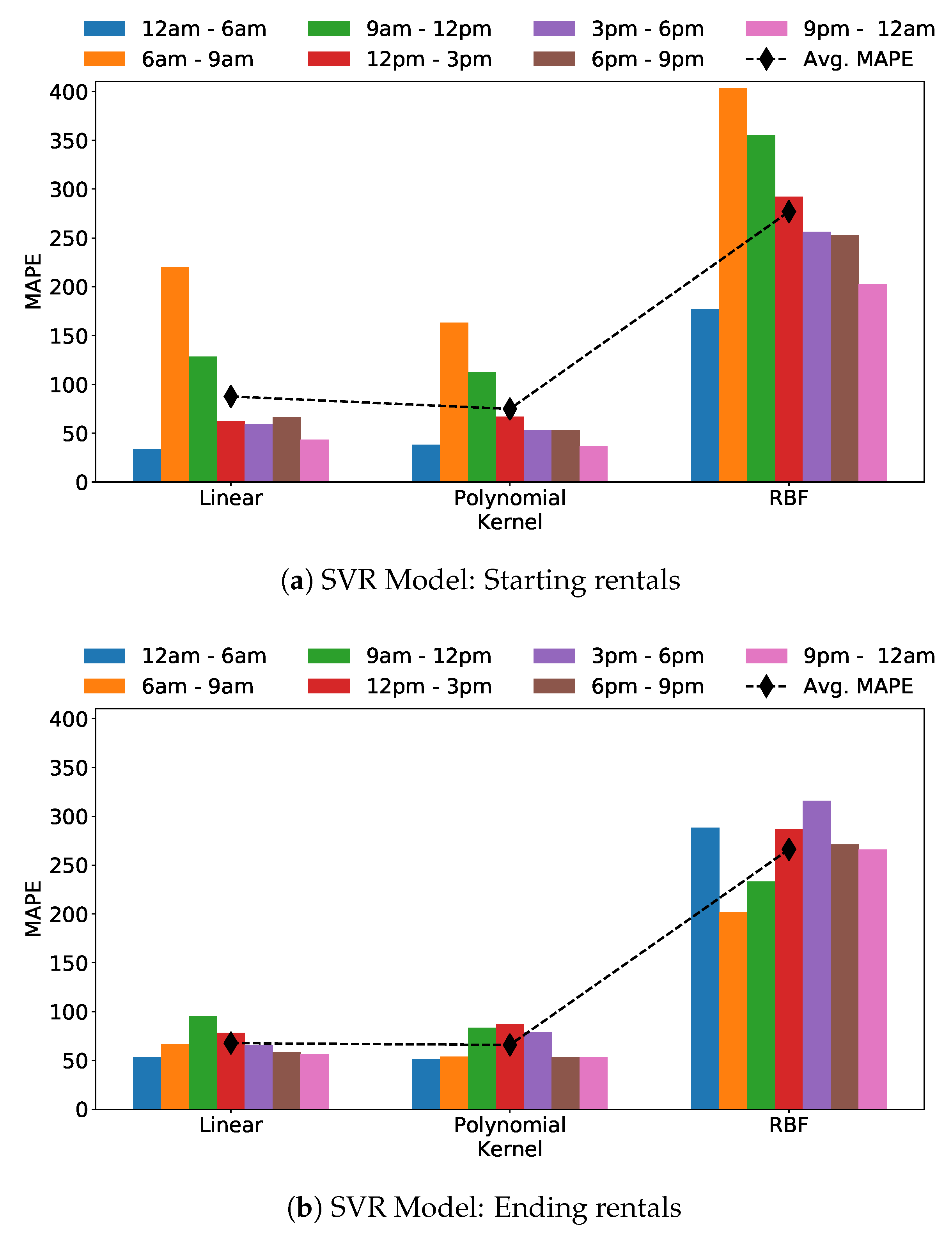
Figure 10a and Figure 11b show the SVR prediction accuracy for the task of predicting the number of starting and ending rentals, respectively. For each kernel type and for each time bin, we report the average MAPE over the 22 experiments (one for each neighborhood that is left out during training). The SVR model performs rather poorly regardless of the parameter setting. Considering the targeted time bin, errors are higher for the morning slots, independently of the kernel, while the time bin from 0 am to 6 am is the one for which the model achieves the best performance. The polynomial kernel performs the best: yet the average (over all time bins) MAPE is 70% for the prediction of starting rentals, and 64% for the prediction of ending rentals. For the sake of completeness, best RMSE for starting and ending rentals predictions are 499.776 and 427.675, respectively, both for time bin from 0 am to 6 am.
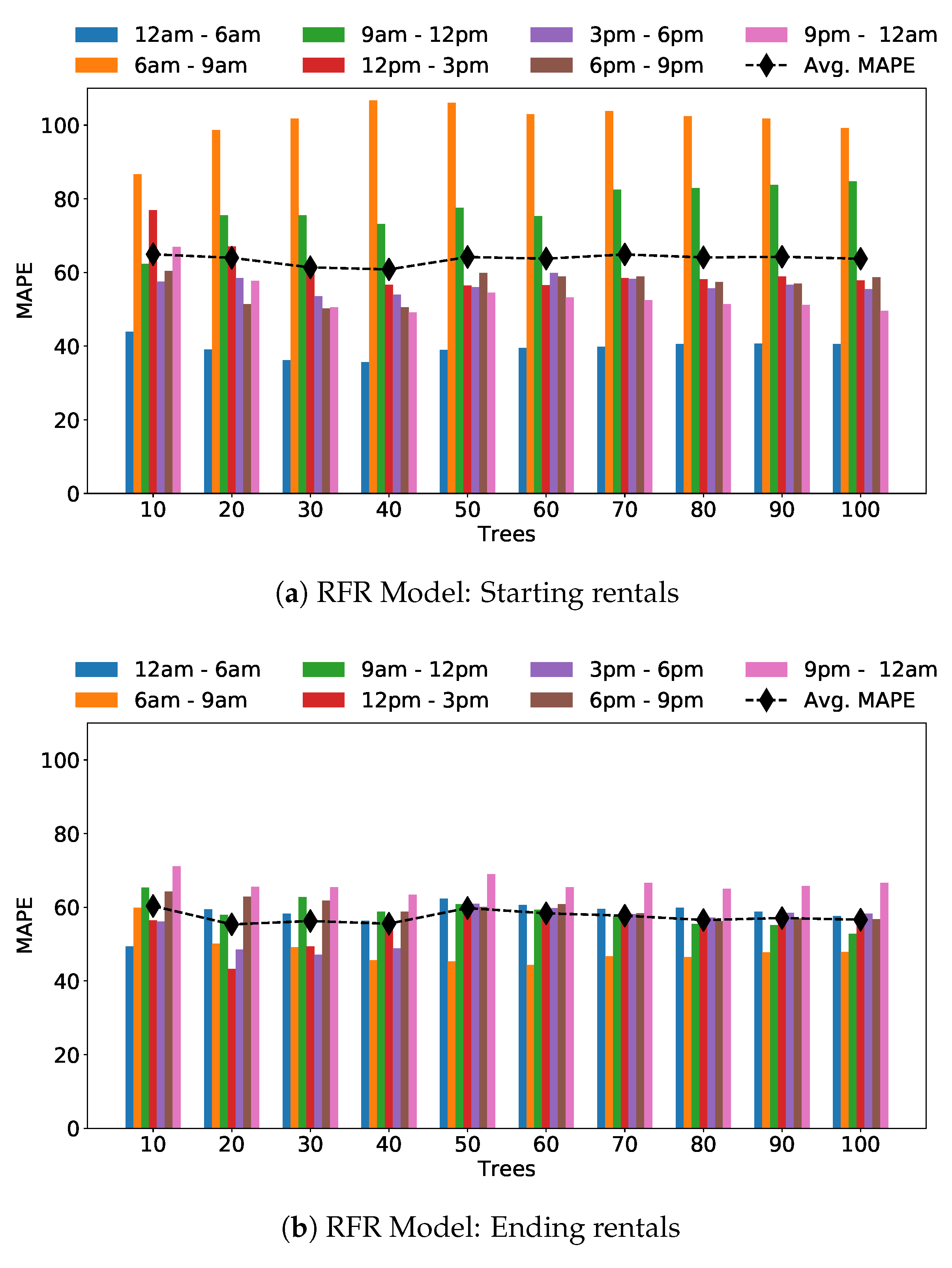
The results for the Random Forest Regression model are shown in Figure 11a,b, for different number of trees. For a given time bin, we observe limited variation in the MAPE for increasing number of trees, which suggests that a small number of trees (30 or 40 trees, for instance) could be enough. This is expected given again the limited number of samples for the training. In this case, the overall MAPE is 59%.
Moving to the predictions for ending rentals in Figure 11b, we observe smaller errors, with the best case with 20 or 40 trees, with the overall MAPE being 56%. Again, in the time bin from 0 am to 6 am we obtain the best predictions while the worst are obtained from 6 am to 9 am (for starting rentals prediction). Regarding RMSE measure, the best value for starting rentals is 427.260 for time from 0 am to 6 am and 50 trees, while for final rentals the best RMSE is 732.825 for time bin 6 am to 9 am.
Overall, the usage of only socio-demographic data as features offers from quite large prediction error. In the following, we investigate which features are the most important so to also perform feature selection and possibly improve the model.
Feature Ranking and Selection
As in the previous section, we here analyze the feature ranking for the RFR model. Table 3 reports the top-15 most relevant features along with their relevance. This feature ranking procedure allows us on the one hand to identify what information the FFCS operator should focus on when considering new neighborhoods of the city in which to implement its service. On the other hand, it allows us to reduce the number of features to use in the model: we can focus only on the most important ones.
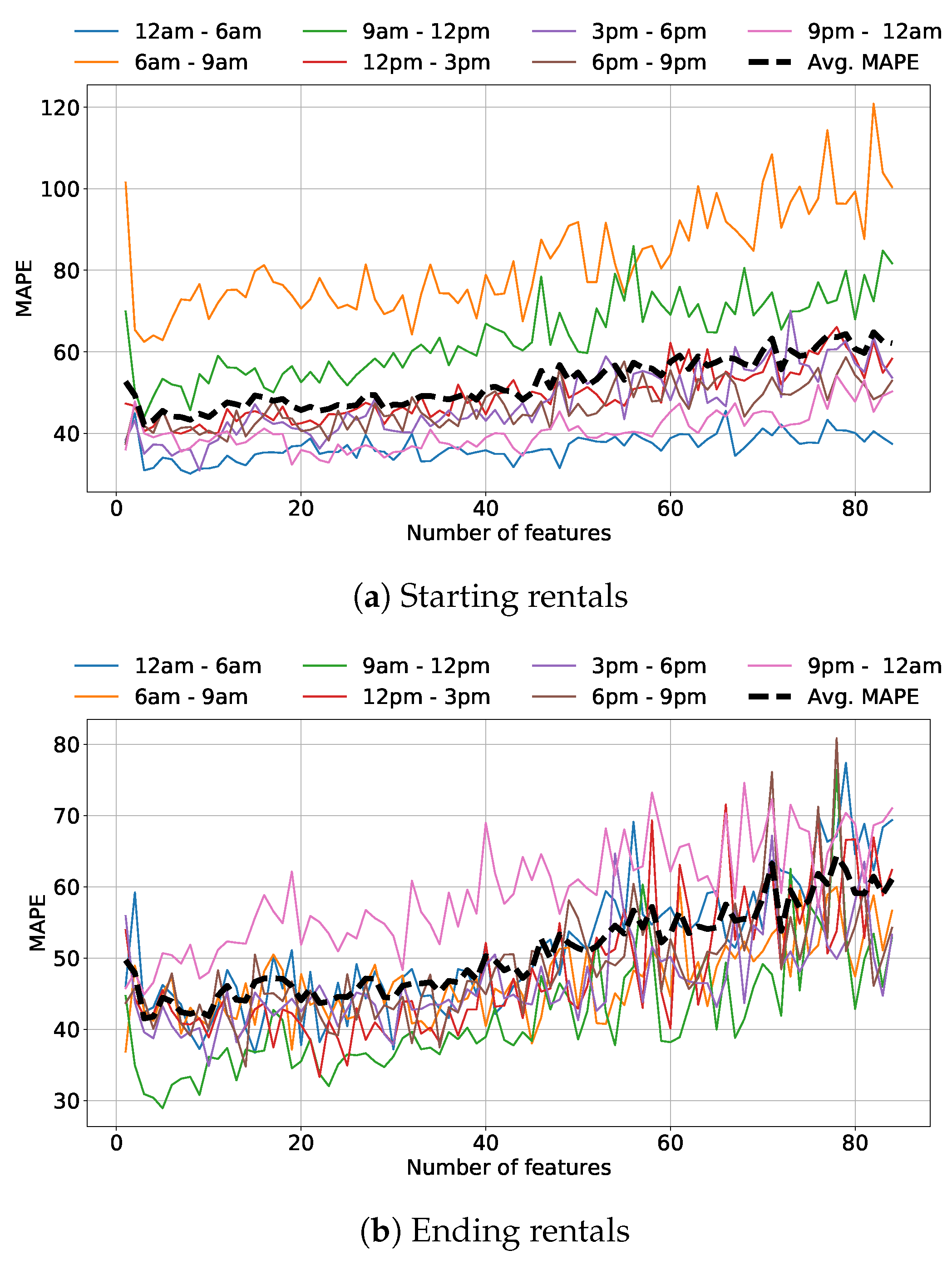
To evaluate the impact of the features on the performance of the model, we train once again the RFR with an increasing number of features, chosen according to the given rank. We fix the number of trees according to the best average MAPE obtained in Figure 11a,b: 40 trees for the starting and 20 for the ending rentals prediction. Figure 12 shows the results. It reports the MAPE versus the number of features in the model. Notice the U-shaped curve of the average MAPE (dashed black line). Intuitively, too few features worsen the regression performance due to lack of information, but too many features reduce the performance since the training is more complicated and the model gets confused.
We further evaluate the RFR model by selecting the best number of features (the one that minimizes the average MAPE), which results to selecting the top 7 features in Table 1. With this subset, the average MAPE is 41% and RMSE equals to 1104.501 for starting rentals, while for arrivals MAPE is 39% and RSME is equal to 1010.453. As expected, using only the most important features significantly improves the performance.
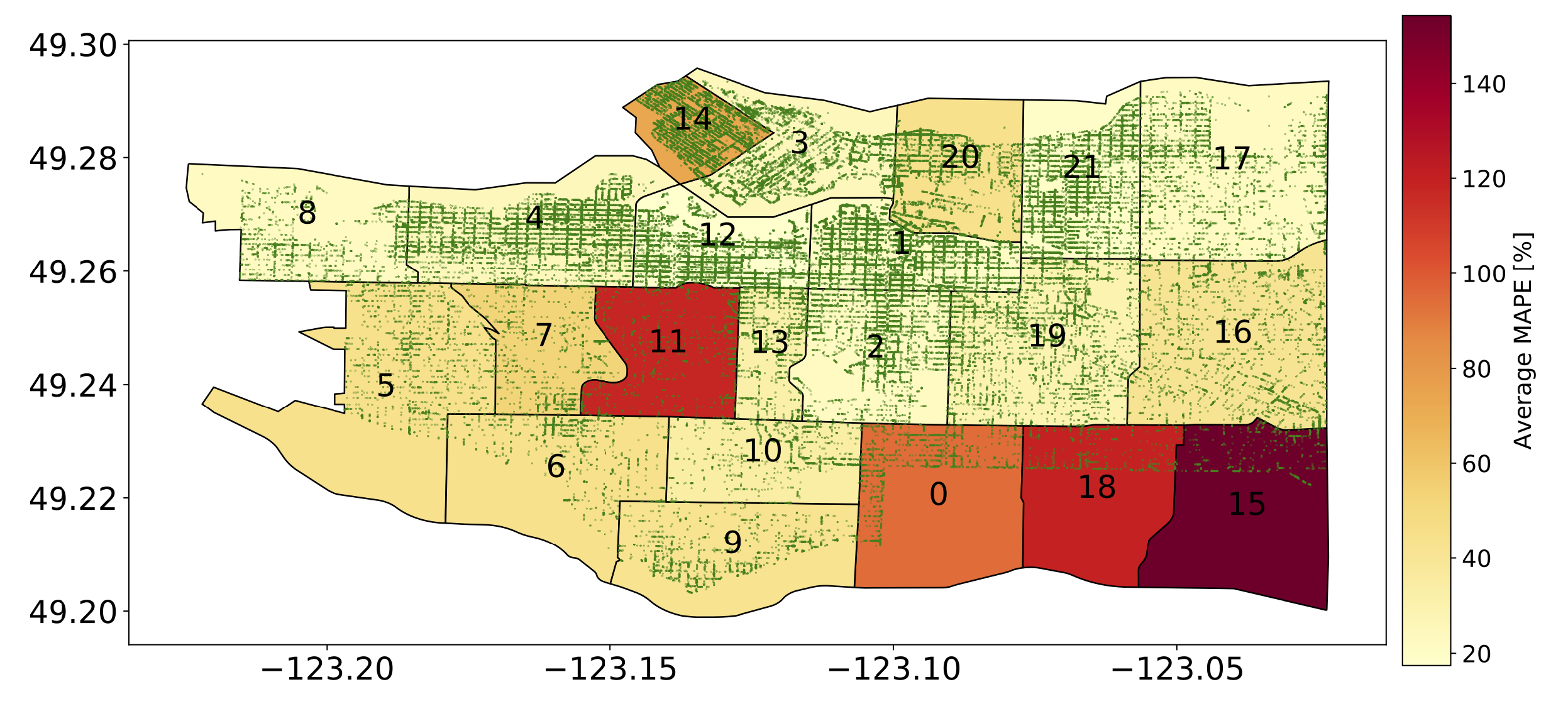
Finally, we explore the spatial prediction error, i.e., we look if there are neighborhoods that present significantly higher errors than others. Figure 13 depicts the heatmap of the MAPE per neighborhood, averaged over all time bins. The more the area is red the higher the average MAPE is. Each green dot represents actual positions of starting or arrival rentals as recorded in the original trace. The neighborhoods with the highest error are the ones labeled 15, 18, 11, and 0. We can see that neighborhoods 15, 18, and 0 are in the periphery and intersect only partially with the rental area of the FFCS operator. This mismatch confuses the prediction since our model assumes the operative area coincides with the total area of each neighborhood. Thus, our model predicts much higher numbers of rentals (reflecting the whole neighborhood area) than the ones that are actually done (reflecting the restricted operational area). Neighborhood 0 has instead a large presence of parks where clearly the car cannot operate. As such, the features of this area are also not reflecting the entire area, fooling the classifier.
In general, the performance of the spatial predictions is lower when compared to the temporal predictions. This is expected given the nature of the problem, the limited amount of available data, and because the number of rentals varies widely within each neighborhood. However, we would like to emphasize that the results of the spatial prediction could be quite useful: the ranking of the regions in terms of service demand is indeed preserved in the predictions. In other words, the neighborhood with the largest demands, which could be the preferred locations to extend the service, would still be predicted correctly.
7. Conclusions
In this paper, we studied the problem of predicting FFCS demand patterns in time and space, a relevant problem to an adequate provisioning of the service and maintenance of the fleet. Relying on data from real FFCS rides in Vancouver as well as the municipality socio-demographic information, we investigated to which extent modern machine-learning-based solutions allow us to predict the transportation demand.
Our results show that the temporal prediction of rentals can be performed with relative errors down to 10%. In this scenario, a Random Forests Regression performs consistently among the best models, and allowing us to also discover which features are more useful for prediction. When considering the spatial prediction using socio-demographic data, we obtain relative errors around 40%, after feature selection. This is expected due to the scarcity of data, but the prediction results are still useful. Indeed, since the number of rentals varies widely within each neighborhood, the relative ranking is preserved. This is valuable for, e.g., looking for the area where to first extend the service. Again, using a Random Forest Regression model, we can observe which features are the most useful for the prediction, a precious information for providers and regulators that wish to understand FFCS systems and to provide a high-quality service that benefits both providers and its costumers.
As future work, we would like to investigate whether this same strategy generalizes to different cities. Answering this question is challenging due to the heterogeneity and diversity of open data in different cities, and of usage patterns of car sharing around the world. We conjecture that given similar data the methodology could be applied to other cities, as there is nothing specific to the analyzed city in it. However, the effectiveness of the models may change depending on peculiarities of each city. Still, it is an open problem towards which we have provided an important first step.
Author Contributions
M.C. and D.T. worked in the software implementation and experimental validation of this work. M.C., D.T., L.V., M.M., J.M.A., and A.P.C.d.S. worked in the conceptualization and definition of the problem, and contributed to the writing and draft preparation. All authors have read and agreed to the published version of the manuscript.
Funding
The research leading to these results has been funded by the Compagnia di San Paolo through the 2019 internationalisation project program between Politecnico di Torino (Italy) and Universidade Federal de Minas Gerais (Brazil), by the Brazilian research agencies CNPq, CAPES and FAPEMIG, and by the SmartData@Polito center.
Conflicts of Interest
The authors declare no conflict of interest.
References
- Litman, T. Evaluating Carsharing Benefits. Transp. Res. Rec. 2000, 1702, 31–35. [Google Scholar] [CrossRef]
- Firnkorn, J.; Müller, M. What will be the environmental effects of new free-floating car-sharing systems? The case of car2go in Ulm. Ecol. Econ. 2011, 70, 1519–1528. [Google Scholar] [CrossRef]
- Firnkorn, J.; Müller, M. Selling mobility instead of cars: New business strategies of automakers and the impact on private vehicle holding. Bus. Strategy Environ. 2012, 21, 264–280. [Google Scholar] [CrossRef]
- Ciari, F.; Weis, C.; Balac, M. Evaluating the influence of carsharing stations’ location on potential membership: A Swiss case study. EURO J. Transp. Logist. 2016, 5, 345–369. [Google Scholar] [CrossRef]
- Cocca, M.; Giordano, D.; Mellia, M.; Vassio, L. Free Floating Electric Car Sharing: A Data Driven Approach for System Design. IEEE Trans. Intell. Transp. Syst. 2019, 1–13. [Google Scholar] [CrossRef]
- Cocca, M.; Giordano, D.; Mellia, M.; Vassio, L. Free floating electric car sharing design: Data driven optimisation. Pervasive Mob. Comput. 2019, 55, 59–75. [Google Scholar] [CrossRef]
- Ciociola, A.; Cocca, M.; Giordano, D.; Mellia, M.; Morichetta, A.; Putina, A.; Salutari, F. UMAP: Urban Mobility Analysis Platform to Harvest Car Sharing Data. In Proceedings of the IEEE Smart City Innovations, San Francisco, CA, USA, 4–8 August 2017. [Google Scholar]
- Brockwell, P.J.; Davis, R.A. Introduction to Time Series and Forecasting; Springer: Berlin/Heidelberg, Germany, 2016. [Google Scholar]
- Bishop, C.M. Pattern Recognition and Machine Learning (Information Science and Statistics); Springer: Berlin/Heidelberg, Germany, 2006. [Google Scholar]
- Okutani, I.; Stephanedes, Y.J. Dynamic prediction of traffic volume through Kalman filtering theory. Transp. Res. Part B Methodol. 1984, 18, 1–11. [Google Scholar] [CrossRef]
- Clark, S. Traffic prediction using multivariate nonparametric regression. J. Transp. Eng. 2003, 129, 161–168. [Google Scholar] [CrossRef]
- Ciari, F.; Schuessler, N.; Axhausen, K.W. Estimation of carsharing demand using an activity-based microsimulation approach: Model discussion and some results. Int. J. Sustain. Transp. 2013, 7, 70–84. [Google Scholar] [CrossRef] [Green Version]
- Catalano, M.; Casto, B.L.; Migliore, M. Car sharing demand estimation and urban transport demand modelling using stated preference techniques. Eur. Transp. 2008, 40, 33–50. [Google Scholar]
- Becker, H.; Ciari, F.; Axhausen, K.W. Comparing car-sharing schemes in Switzerland: User groups and usage patterns. Transp. Res. Part A Policy Pract. 2017, 97, 17–29. [Google Scholar] [CrossRef] [Green Version]
- Schmöller, S.; Bogenberger, K. Analyzing external factors on the spatial and temporal demand of car sharing systems. Procedia-Soc. Behav. Sci. 2014, 111, 8–17. [Google Scholar] [CrossRef] [Green Version]
- Schmöller, S.; Weikl, S.; Müller, J.; Bogenberger, K. Empirical analysis of free-floating carsharing usage: The Munich and Berlin case. Transp. Res. Part C Emerg. Technol. 2015, 56, 34–51. [Google Scholar] [CrossRef]
- Alencar, V.A.; Rooke, F.; Cocca, M.; Vassio, L.; Almeida, J.; Vieira, A.B. Characterizing client usage patterns and service demand for car-sharing systems. Inform. Syst. 2019. [Google Scholar] [CrossRef]
- He, S.; Shin, K.G. Spatio-temporal Adaptive Pricing for Balancing Mobility-on-Demand Networks. ACM Trans. Intell. Syst. Technol. 2019, 10, 39:1–39:28. [Google Scholar] [CrossRef] [Green Version]
- Hulot, P.; Aloise, D.; Jena, S.D. Towards Station-Level Demand Prediction for Effective Rebalancing in Bike-Sharing Systems. In Proceedings of the 24th ACM SIGKDD International Conference on Knowledge Discovery & Data Mining, KDD ’18, London, UK, 19–23 August 2018; ACM: New York, NY, USA, 2018; pp. 378–386. [Google Scholar] [CrossRef] [Green Version]
- Wang, D.; Cao, W.; Li, J.; Ye, J. DeepSD: Supply-demand prediction for online car-hailing services using deep neural networks. In Proceedings of the 2017 IEEE 33rd International Conference on Data Engineering (ICDE), San Diego, CA, USA, 19–22 April 2017; pp. 243–254. [Google Scholar]
- Jain, R. The Art of Computer Systems Performance Analysis: Techniques for Experimental Design, Measurement, Simulation, and Modeling; John Wiley & Sons: Hoboken, NJ, USA, 1990. [Google Scholar]
- Pedregosa, F.; Varoquaux, G.; Gramfort, A.; Michel, V.; Thirion, B.; Grisel, O.; Blondel, M.; Prettenhofer, P.; Weiss, R.; Dubourg, V.; et al. Scikit-learn: Machine Learning in Python. J. Mach. Learn. Res. 2011, 12, 2825–2830. [Google Scholar]
Figure 1.
Time series of starting rentals in September 2017 aggregated per hour. The difference in the total number of time bins and the actual number of hours in the month are due to missing data (crawler failures).
Figure 1.
Time series of starting rentals in September 2017 aggregated per hour. The difference in the total number of time bins and the actual number of hours in the month are due to missing data (crawler failures).

Figure 2.
Temporal characterization of number of rentals. Box-plots highlighting the variability over the day for the same time bin of the day (top plots), and over different days (bottom plots).
Figure 2.
Temporal characterization of number of rentals. Box-plots highlighting the variability over the day for the same time bin of the day (top plots), and over different days (bottom plots).

Figure 3.
Heatmap of net flow for each neighborhood in Vancouver. The more the area is red, the higher are the arrivals with respect to the departures. Neighborhood numbering is shown (from 0 to 21).
Figure 3.
Heatmap of net flow for each neighborhood in Vancouver. The more the area is red, the higher are the arrivals with respect to the departures. Neighborhood numbering is shown (from 0 to 21).

Figure 4.
Total net flow in September 2017 for Downtown (neighborhood 3) and Grandview-Woodland (neighborhood 21) over different hours of the day.
Figure 4.
Total net flow in September 2017 for Downtown (neighborhood 3) and Grandview-Woodland (neighborhood 21) over different hours of the day.

Figure 5.
Time series of weather conditions per hour during September 2017. Each point in the plot represents an occurred weather type.
Figure 5.
Time series of weather conditions per hour during September 2017. Each point in the plot represents an occurred weather type.

Figure 6.
Heatmap of a sample of demographic (a) and socio-demographic (b) data at our disposals. These two samples look quite correlated.
Figure 6.
Heatmap of a sample of demographic (a) and socio-demographic (b) data at our disposals. These two samples look quite correlated.

Figure 7.
Long-term temporal prediction—Performance of the RFR model in one month of the validation set. The difference in the total number of time bins and the actual number of hours in the month are due to missing data (crawler failures).
Figure 7.
Long-term temporal prediction—Performance of the RFR model in one month of the validation set. The difference in the total number of time bins and the actual number of hours in the month are due to missing data (crawler failures).

Figure 8.
Effect of the number of epochs on the performance (MAPE) of the Neural Networks model.

Figure 9.
Short-term temporal prediction—Performance of the RFR model with expanding window in the validation set (24 days).
Figure 9.
Short-term temporal prediction—Performance of the RFR model with expanding window in the validation set (24 days).

Figure 10.
Spatial prediction—MAPE for Support Vector Regression models, using different kernels.

Figure 11.
Spatial prediction—MAPE for Random Forests Regression models, using different number of trees.
Figure 11.
Spatial prediction—MAPE for Random Forests Regression models, using different number of trees.

Figure 12.
Spatial prediction—MAPE in the different time bins by selecting the most relevant features in RFR.
Figure 12.
Spatial prediction—MAPE in the different time bins by selecting the most relevant features in RFR.

Figure 13.
Spatial distribution—Heatmap of average MAPE per neighborhood. Rentals are shown on the map as green points.
Figure 13.
Spatial distribution—Heatmap of average MAPE per neighborhood. Rentals are shown on the map as green points.


Table 1.
Long-term temporal prediction—Mean Absolute Percentage Error (MAPE), Standard Deviation of the Absolute Percentage Error (APE) and Root Mean Square Error (RMSE) for each prediction model in the validation set.
Table 1.
Long-term temporal prediction—Mean Absolute Percentage Error (MAPE), Standard Deviation of the Absolute Percentage Error (APE) and Root Mean Square Error (RMSE) for each prediction model in the validation set.
| Prediction Model | MAPE [%] | (APE) [%] | RMSE |
|---|---|---|---|
| Baseline | 40.05 | 44.95 | 321.32 |
| ARIMA | 25.53 | 19.68 | 238.87 |
| SARIMA | 21.15 | 21.74 | 159.17 |
| Linear Regression | 15.80 | 15.61 | 178.57 |
| Support Vector Regression | 15.12 | 16.14 | 179.99 |
| Random Forest Regression | 14.63 | 11.62 | 157.40 |
| Neural Networks | 15.83 | 16.60 | 187.08 |
Table 2.
Short-term temporal prediction—Mean Absolute Percentage Error (MAPE), Absolute Percentage Error (APE), and Root Mean Squared Error (RMSE), for each prediction model in the validation set.
Table 2.
Short-term temporal prediction—Mean Absolute Percentage Error (MAPE), Absolute Percentage Error (APE), and Root Mean Squared Error (RMSE), for each prediction model in the validation set.
| Prediction Model | Expanding Window (Starting: 28 Days) | Sliding Window (28 Days) | ||||
|---|---|---|---|---|---|---|
| MAPE [%] | (APE) [%] | RMSE | MAPE [%] | (APE) [%] | RMSE | |
| Baseline | 20.12 | 16.64 | 195.53 | 20.12 | 16.64 | 195.53 |
| ARIMA | 36.01 | 35.87 | 306.80 | 36.52 | 36.60 | 305.50 |
| SARIMA | 17.60 | 20.01 | 160.42 | 18.02 | 21.75 | 163.94 |
| Linear Regression | 18.28 | 20.38 | 179.11 | 18.11 | 20.55 | 178.61 |
| Support Vector Regression | 12.22 | 15.62 | 128.72 | 12.87 | 18.52 | 136.14 |
| Random Forests Regression | 9.71 | 8.34 | 104.99 | 10.08 | 12.23 | 109.47 |
| Neural Networks | 10.52 | 12.93 | 128.84 | 10.52 | 12.74 | 123.55 |
Table 3.
Spatial prediction—Most relevant features and their importance for the prediction using Random Forest Regression. The first 7 are the ones that for obtain the best overall model.
Table 3.
Spatial prediction—Most relevant features and their importance for the prediction using Random Forest Regression. The first 7 are the ones that for obtain the best overall model.
| Rank | Feature | Relevance |
|---|---|---|
| 1 | Number of emergency calls | 0.0717 |
| 2 | Distance from downtown | 0.0481 |
| 3 | People commuting by walk | 0.0381 |
| 4 | People commuting within Vancouver | 0.0342 |
| 5 | People with income between 100,000 and 149,999 $CAD | 0.0298 |
| 6 | People with income between 60,000 and 69,999 $CAD | 0.0286 |
| 7 | People legally recognized as couple | 0.0281 |
| 8 | People with income more than 150,000 $CAD | 0.0274 |
| 9 | People divorced | 0.0261 |
| 10 | People commuting within the same neighborhood | 0.0249 |
| 11 | Couples with more than 3 children | 0.0239 |
| 12 | People with age between 50 and 54 years | 0.0233 |
| 13 | Unemployed people | 0.0231 |
| 14 | People never married | 0.0217 |
| 15 | People with income between 80,000 and 89,999 $CAD | 0.0211 |
© 2020 by the authors. Licensee MDPI, Basel, Switzerland. This article is an open access article distributed under the terms and conditions of the Creative Commons Attribution (CC BY) license (http://creativecommons.org/licenses/by/4.0/).
Share and Cite
MDPI and ACS Style
Cocca, M.; Teixeira, D.; Vassio, L.; Mellia, M.; Almeida, J.M.; Couto da Silva, A.P. On Car-Sharing Usage Prediction with Open Socio-Demographic Data. Electronics 2020, 9, 72. https://0-doi-org.brum.beds.ac.uk/10.3390/electronics9010072
AMA Style
Cocca M, Teixeira D, Vassio L, Mellia M, Almeida JM, Couto da Silva AP. On Car-Sharing Usage Prediction with Open Socio-Demographic Data. Electronics. 2020; 9(1):72. https://0-doi-org.brum.beds.ac.uk/10.3390/electronics9010072
Chicago/Turabian StyleCocca, Michele, Douglas Teixeira, Luca Vassio, Marco Mellia, Jussara M. Almeida, and Ana Paula Couto da Silva. 2020. "On Car-Sharing Usage Prediction with Open Socio-Demographic Data" Electronics 9, no. 1: 72. https://0-doi-org.brum.beds.ac.uk/10.3390/electronics9010072
Note that from the first issue of 2016, this journal uses article numbers instead of page numbers. See further details here.