Mixed Finite Element Simulation with Stability Analysis for Gas Transport in Low-Permeability Reservoirs

Abstract

Natural gas exists in considerable quantities in tight reservoirs. Tight formations are rocks with very tiny or poorly connected pors that make flow through them very difficult, i.e., the permeability is very low. The mixed finite element method (MFEM), which is locally conservative, is suitable to simulate the flow in porous media. This paper is devoted to developing a mixed finite element (MFE) technique to simulate the gas transport in low permeability reservoirs. The mathematical model, which describes gas transport in low permeability formations, contains slippage effect, as well as adsorption and diffusion mechanisms. The apparent permeability is employed to represent the slippage effect in low-permeability formations. The gas adsorption on the pore surface has been described by Langmuir isotherm model, while the Peng-Robinson equation of state is used in the thermodynamic calculations. Important compatibility conditions must hold to guarantee the stability of the mixed method by adding additional constraints to the numerical discretization. The stability conditions of the MFE scheme has been provided. A theorem and three lemmas on the stability analysis of the mixed finite element method (MFEM) have been established and proven. A semi-implicit scheme is developed to solve the governing equations. Numerical experiments are carried out under various values of the physical parameters.

1. Introduction

Natural gas was formed in tight formations over millions of years, when organic material was buried under high heat and pressure and slowly converted to natural gas. Some of this natural gas escaped into the adjacent conventional rock layers with higher porosity and permeability, and is relatively easy to extract. However, the majority remained locked in tighter, lower permeability layers where they could not be extracted through conventional means. In tight-gas formations, micro-, and nano-pores, the no-slip surface condition may not be satisfied and flow slippage may take place. Due to the gas slippage effect, the permeability of a sample to a gas varies with the molecular weight of the gas and the applied pressure, which was first proposed by Klinkenberg [1], i.e., the so-called Klinkenberg effect. This non-Darcy Klinkenberg effect occurs when the mean free path length of the gas molecules is close to the average size of pores. This condition results in the acceleration of individual gas molecules along the flow path [2]. In recent years, the Klinkenberg effect gains more attractions with the development of shale gas [3]. Wu et al. [4] have developed some analytical solutions for analyzing steady-state and transient gas flow through porous media including Klinkenberg effects. Other popular approaches such as those by Pazos et al. [5], and Esmaili and Mohaghegh [6] consider the determination of the shale gas permeability. Javadpour et al. [7] and Javadpour [8] have described the fluid flow and transport in a shale matrix by Knudsen diffusion and slip flow in the nanopores, desorption from the surface of kerogen, and diffusion in solid kerogen. Cui et al. [9] have introduced some measurements of gas permeability and diffusivity of the tight reservoir rocks using different approaches. Shabro et al. [10] have presented numerical simulation of shale-gas production including pore-scale modeling of slip-flow, Knudsen diffusion, and Langmuir desorption and reservoir modeling of compressible fluid. A study on shale-gas permeability and diffusivity inferred by improved formulation of relevant retention and transport mechanisms has been introduced by Civan et al. [11]. Freeman et al. [12] have investigated gas composition changes in shale gas well. Recently, screening improved recovery methods in tight-oil formations by injecting and producing through fractures, have been presented by Singh and Cai [13]. Ge et al. [14] have investigated organic related pores in unconventional reservoir and its quantitative evaluation. Nanoporous structure and gas occurrence of organic-rich shales have been studied by Qi et al. [15]. Salama et al. [16] have presented an intensive review on the recent advances of the flow and transport phenomena in tight and shale formation. El-Amin et al. [17] have introduced a comparative study of transport of shale-gas in fractured porous media. El-Amin et al. [18,19] have presented analytical solutions using the power-series method for the apparent permeability and fractional derivative gas-transport equation in porous media.

Simulation of transport phenomena in tight geological media demands high accuracy and local mass conservation to be able to handle the dramatic change in spatial and temporal scales. Some numerical approximation schemes fail to preserve important physical and/or mathematical principles and lead to erroneous simulation results. For example, the continuous Galerkin finite element method is not locally mass conservative, while the mixed finite element methods (MFEM) [20,21,22,23,24,25] are all locally conservative. The mixed method is based on the conservation law together with the constitutive law for the flux in terms of pressure and solving the flux and the pressure together. Since this preserves the structure of the equations, this approach is consistent with the required properties of the numerical methods. In addition, the MFE schemes can be extended to a higher-order approximation easily. Moreover, in the MFEM, the approximation to velocity can be more accurate than the approximation to pressure. For example, in the lowest order Brezzi–Douglas–Marini (BDM1) mixed finite element method space, an enhanced linear space has been used for velocity approximation, while a piece-wise constant space has been used for pressure approximation. In general, the finite element methods can handle unstructured mesh.

This paper presents a model to simulate the transport of gas in tight permeability formations considering slippage, adsorption, and diffusion effects. The mixed finite element method (MFEM) was applied and its stability analyzed. A theoretical foundation of the stability analysis is provided. Numerical experiments are also provided and selected results are presented. The rest of the paper is organized as follows. In Section 2, the mathematical model of the problem under consideration is described. The solution method is presented in Section 3: mathematical preliminaries are introduced in Section 3.1; the mixed finite element method of the current problem is given in Section 3.2; and the numerical algorithm is presented in Section 3.3. Section 4 considers the stability analysis, while numerical discussions are presented in Section 5. Finally, conclusions are drawn in Section 6.

2. Modeling and Formulation

In this section, the model of a single equation to simulate the transport of gas in tight permeability formations has been developed with considering slippage, adsorption and diffusion effects. In low-permeability formations, the Klinkenberg effect takes place and the apparent permeability model has been used to describe this effect. The cubic Peng-Robinson equation of state to compute the gas deviation factor has been employed. In this study, it has been assumed that the flow is a single-phase and isothermal, and the gravity is neglected. The mass accumulation of the adsorbed gas on the surface is described by the Langmuir isotherm model [9,10,11,12], as,

$$q_a=\frac{(1-\varphi ){\rho }_s{M}_w{V}_{L}p}{V_{std}(P_L+p)}$$

(1)

where $V_{std}$ (m${}^3$ mol${}^{-1}$) is the mole volume under standard conditions; $V_L$ (m${}^3$ kg${}^{-1}$) is the Langmuir volume; $P_L$ (Pa) is the Langmuir pressure; ${\rho }_s$ (kg m${}^{-3}$) is the density of the shale core; p (Pa) is the pressure; and $M_w$ (kg mol${}^{-1}$) is the molar weight. Manipulating the time derivative of the adsorbed mass, Equation (1), such that,

$$\frac{\partial q_a}{\partial t}=\frac{\partial q_a}{\partial p}\frac{\partial p}{\partial t}=\frac{{\rho }_s{M}_w{V}_L{P}_L}{V_{\mathit{std}}(P_L{+p)}^2}\frac{\partial p}{\partial t}.$$

(2)

The mass accumulation of both free and absorbed gas is given by, $M=\varphi \rho +(1-\varphi )q_a$, and the mass density can be written as,

$$\rho =\frac{p{M}_w}{ZRT}.$$

(3)

To compute the gas deviation factor, Z, the cubic Peng-Robinson equation of state is employed, which can be expressed as follows [25],

$$Z^3-(1-\mathrm{B}){\mathrm{Z}}^2+(\mathrm{A}-3{\mathrm{B}}^3-2\mathrm{B})\mathrm{Z}-(\mathrm{AB}-{\mathrm{B}}^2-{\mathrm{B}}^3)=0$$

(4)

where

$$\mathrm{A}=\frac{{\mathrm{a}}_{T}p}{R^2{T}^2},\mathrm{B}=\frac{{\mathrm{b}}_{T}p}{RT}.$$

(5)

The coefficients ${\mathrm{a}}_T$ and ${\mathrm{b}}_T$ are functions of the critical properties, thus,

$${\mathrm{a}}_T=0.45724\frac{R^2{T}_{\mathrm{c}}^2}{p_{\mathrm{c}}},{\mathrm{b}}_T=0.0778\frac{{RT}_{\mathrm{c}}}{p_{\mathrm{c}}}.$$

(6)

The slippage factor rectifies the slippage effect on permeability measurements. In low-permeability formations or under low-pressure condition, the Klinkenberg effect takes place and the apparent permeability is expressed as a function of the gas pressure,

$$k_{app}=k_0(1+\frac{\mathrm{b}}{p}),$$

(7)

where b (Pa) is the Klinkenberg slippage factor which is a function of the gas molecule slippage along the pore walls at low values of pore pressure, and $k_0$ (m${}^3$) is the intrinsic permeability value. The Klinkenberg slippage factor b, can be written as [7,8],

$$\mathrm{b}=\sqrt{\frac{8\pi RT}{M_w}}\frac{1}{r}\left(\frac{2}{\alpha }-0.995\right)\mu .$$

(8)

From the definition of b, one may notice that the coefficient b depends on both T (K) and $\mu$ (Pa s), however, in the current study, it was assumed that the system is isothermal and $\mu$ is constant, so the value of b becomes constant. The variation of T and $\mu$ may be considered in a future work. The Klinkenberg effect may express the pore geometry difference between conventional and tight reservoirs as given by Equation (7). At very high pressure, the slippage effect disappears as a result and the gas behavior. In order to simplify the model, it is assumed that the flow in the shale reservoir is a single-phase and isothermal, while the gravity is neglected. On the other hand, Brown et al. [26] presented the theoretical coefficient, $F=1+\sqrt{8\pi \gamma }\frac{\mu }{rp}(\frac{2}{\alpha }-1)$, to correct the slip velocity in a tube. It is clear from this formula that $\alpha$ has an opposite effect on the slip effect which, in turn, improves the flow on the boundary. This may interpret the previous observation. Javadpour et al. [7] have reported that $\alpha$ = 0.8 to fit with the experimental data by Rot et al. [27]. In addition, El-Amin et al. [17] have constructed model which gives a good match with experimental results [27] for the same value of $\alpha$ = 0.8.

Using the general mass balance equation, the governing equation is stated as,

$$f_1\left(p\right)\frac{\partial p}{\partial t}-\nabla ·\left[\frac{\rho \left(p\right)}{\mu }{k}_0\left(1+\frac{b}{p}\right)\nabla p\right]=-Q\left(p\right),$$

(9)

where $\varphi$ is the medium porosity and

$$f_1\left(p\right)=\frac{M_w\varphi }{ZRT}+\frac{M_w{V}_L{\rho }_s}{V_{std}}\frac{P_L(1-\varphi )}{{(P_L+p)}^2}.$$

(10)

The production well source is represented by,

$$Q\left(p\right)=\frac{\theta \rho k}{\mu ln\frac{re}{r_w}}\left(p_e-p_w\right),$$

(11)

where $r_w$ (m) is the well radius. If the production well is located in the center, $\theta =2\pi$, while, if the production well is located in the corner, $\theta =\pi /2$. $p_e$ (Pa) is the average pressure around the well. $r_e$ (m) is the drainage radius, which is defined by,

$$r_e=r_{\mathrm{c}}\sqrt{{(\Delta x)}^2+{(\Delta y)}^2},$$

(12)

such that $r_{\mathrm{c}}$ is a constant and $\Delta x,\Delta y$ are the $x-,y-$ space mesh size, respectively.

The initial conditions are

$$p(·,0)=p_0\mathrm{in}\mathsf{\Omega }.$$

(13)

The boundary conditions are

$$p(·,t)=p_w\mathrm{on}{\mathsf{\Gamma }}_D\times (0,T),$$

(14)

$$\mathbf{u}·\mathbf{n}=0\mathrm{on}{\mathsf{\Gamma }}_N\times (0,T).$$

(15)

3. Method of Solution

The model of transport in porous media is usually described by a parabolic system with two natural variables, a scalar variable and its flux, each of them belongs to a different space. The mixed finite element method was developed to approximate the two variables simultaneously. Important compatibility conditions must hold for the two finite element spaces to guarantee the stability, the consistency and the convergence of the mixed method. These requirements are based on properties of the governing partial differential equations. In the following, some preliminaries have presented about the finite element spaces that used in the MFEM analysis.

3.1. Preliminaries

Let the polygonal/polyhedral Lipschitz connected domain $\mathsf{\Omega }\subset {\mathbb{R}}^d,d\in \{1,2,3\}$, with the smooth boundaries, $\partial \mathsf{\Omega }={\mathsf{\Gamma }}_D\cup {\mathsf{\Gamma }}_N$. Firstly, define the inner product in $\mathsf{\Omega }$ as,

$${(f,g)}_{\mathsf{\Omega }}={\int }_{\mathsf{\Omega }}f\left(\mathbf{x}\right)g\left(\mathbf{x}\right)d\mathbf{x}\forall f,g:\mathsf{\Omega }\to \mathbb{R},$$

(16)

and the inner product on $\partial \mathsf{\Omega }$ is defined as,

$${\langle f,g\rangle }_{\partial \mathsf{\Omega }}={\int }_{\partial \mathsf{\Omega }}fgdS\forall f,g:\partial \mathsf{\Omega }\to \mathbb{R}.$$

(17)

One may denote,

$${\mathbb{L}}^2\left(\mathsf{\Omega }\right)=\{f:\mathsf{\Omega }\to \mathbb{R}:{\int }_{\mathsf{\Omega }}{f}^{2}dx<+\infty \}.$$

(18)

Denote $\parallel ·\parallel$ as the standard norm of ${\mathbb{L}}^2\left(\mathsf{\Omega }\right)$ and ${({\mathbb{L}}^2\left(\mathsf{\Omega }\right))}^d$. The space $\mathbb{H}(div,\mathsf{\Omega })$ is defined as

$$\mathbb{H}(div,\mathsf{\Omega })=\{\mathbf{u}\in {({\mathbb{L}}^2\left(\mathsf{\Omega }\right))}^d:\nabla ·\mathbf{u}\in {\mathbb{L}}^2\left(\mathsf{\Omega }\right)\}.$$

(19)

Furthermore, one may define the norm of $\mathbb{H}(div,\mathsf{\Omega })$ as

$${\parallel \mathbf{u}\parallel }_{\mathbb{H}(div,\mathsf{\Omega })}^2={\parallel \mathbf{u}\parallel }^2+{\parallel \nabla ·\mathbf{u}\parallel }^2.$$

(20)

In the context of the mixed finite element, the pressure and velocity usually belong to ${\mathbb{L}}^2\left(\mathsf{\Omega }\right)$ and $\mathbb{H}(div,\mathsf{\Omega })$, respectively. Therefore, the seeking solution is,

$$(p,\mathbf{u})\in {\mathbb{L}}^2\left(\mathsf{\Omega }\right)\times \mathbb{H}(div,\mathsf{\Omega }).$$

(21)

For numerical discretization, the r-th order ($r\ge 0$) Raviart–Thomas ($R{T}_r$) subspaces [20] are introduced to approximate $\mathbb{H}(div,\mathsf{\Omega })$

$$W_h\subset {\mathbb{L}}^2\left(\mathsf{\Omega }\right),\mathbf{dim}\left(W_h\right)<+\infty ,$$

(22)

$$V_h\subset \mathbb{H}(div,\mathsf{\Omega }),\mathbf{dim}\left(V_h\right)<+\infty .$$

(23)

The condition $V_h\subset \mathbb{H}(div,\mathsf{\Omega })$ translates into a continuity condition over the inter-element boundaries $E\in {\mathcal{E}}_h$ of the mesh ${\mathcal{K}}_h$. In other words, one requires that the normal component $\mathbf{u}·\mathbf{n}$ is continuous across the inter-element boundaries. The velocity ${\mathbf{u}}_h\in V_h$ and the pressure $p_h\in W_h$ are sought.

3.2. Mixed Finite Element Approximation

The main idea of using the MFEM is to separate the equation into two equations, one for the pressure and the other for the velocity. Thus, one may rewrite the governing equation as,

$$f_1\left(p\right)\frac{\partial p}{\partial t}+\nabla ·\mathbf{u}=-Q\left(p\right)\mathrm{in}\mathsf{\Omega }\times (0,T),$$

(24)

$$\mathbf{D}{\left(p\right)}^{-1}\mathbf{u}=-\nabla p\mathrm{in}\mathsf{\Omega }\times (0,T),$$

(25)

where

$$\mathbf{D}\left(p\right)=\frac{\rho k_0}{\mu }\left(1+\frac{\mathrm{b}}{p}\right).$$

(26)

The function $\mathbf{D}\left(p\right)$ has been moved into the left hand side to avoid discontinuity when one integrates $\nabla p$ by parts. Selecting any $\phi \in L^2\left(\mathsf{\Omega }\right)$ and $\omega \in \mathbb{H}(div,\mathsf{\Omega })$, the weak formulation takes the form,

$$\left(f_1\left(p\right)\frac{\partial p}{\partial t},\phi \right)+(\nabla ·\mathbf{u},\phi )=-(Q\left(p\right),\phi ),$$

(27)

$$(\mathbf{D}{\left(p\right)}^{-1}\mathbf{u},\omega )=(p,\nabla ·\omega )-{〈p_w,\omega 〉}_{{\mathsf{\Gamma }}^D}.$$

(28)

Now, let the approximating subspace duality $V_h\subset H(\mathsf{\Omega };div)$ and $W_h\subset L^2\left(\mathsf{\Omega }\right)$ be the r-th order ($r\ge 0$) Raviart–Thomas space (RT${}_r$) on the partition ${\mathcal{T}}_h$. The mixed finite element problem are stated as: Find $p^h\in W_h$ and $u^h\in V_h$ such that,

$$\left(f_1\left(p^h\right)\frac{\partial p^h}{\partial t},\phi \right)+(\nabla ·{\mathbf{u}}^h,\phi )=-(Q(p^h),\phi ),\phi \in W_h,$$

(29)

$$(\mathbf{D}{(p^h)}^{-1}{\mathbf{u}}^h,\omega )=(p^h,\nabla ·\omega )-{〈p_w,\omega 〉}_{{\mathsf{\Gamma }}^D},\omega \in V_h.$$

(30)

3.3. Numerical Algorithm

Dividing the total time interval $[0,T]$ into $N_T$ time steps such that the time step length is $\Delta t^n=t^{n+1}-t^n$. The current time step is represented by the superscript $n+1$, while the previous one is represented by n. The backward Euler time discretization is used for the time derivatives terms in the two equations of pressure. The following semi-implicit scheme has been used for the time discretization.

$$\left(f_1(p^{h,n})\frac{p^{h,n+1}-p^{h,n}}{\Delta t},\phi \right)+(\nabla ·{\mathbf{u}}^{h,n+1},\phi )+(Q(p^{h,n}),\phi )=0,$$

(31)

$$(\mathbf{D}{(p^{h,n})}^{-1}{\mathbf{u}}^{h,n+1},\omega )=(p^{h,n+1},\nabla ·\omega )-{〈p_w,\omega 〉}_{{\mathsf{\Gamma }}^D}.$$

(32)

Assume that $p^{h,n}$ is calculated or provided, the thermodynamical variables have been updated explicitly and in this case, and Equations (31) and (32) are linear. In this work, the RT${}_0$ space on the rectangular mesh is employed. The quadrature rule in the MFE scheme has been used to obtain an explicit formulation of ${\mathbf{u}}^{h,n+1}$, and Equations (31) and (32) have been reduced to an equation of $p^{h,n+1}$ as discretized by the cell-centered finite difference method.

4. Stability Analysis

To ensure that the discrete solutions are bounded in a reasonable range, the stability analysis of the proposed technique has been considered. The nonlinearity of the pressure is considered as a key issue encountered in the stability analysis. Hence, one defines some auxiliary functions and analyze their boundedness. Now, one may define the following two functions,

$$F_1(p^h)={\int }_0^{p^h}{f}_1(p^h)d{p}^h,G_1(p^h)={\int }_0^{p^h}{F}_1(p^h)d{p}^h,$$

(33)

Therefore,

$$F_1(p^h)=\frac{M_w\varphi }{RT}{p}^h-\frac{M_w{V}_L{\rho }_s(1-\varphi )}{V_{std}}{(1+\frac{p^h}{P_L})}^{-1}.$$

(34)

If $p^h<P_L$, and $\frac{p^h}{P_L}<1$, one can use the following expansion,

$${\left(1+\frac{p^h}{P_L}\right)}^{-1}=1-\frac{p^h}{P_L}+{\left(\frac{p^h}{P_L}\right)}^2-{\left(\frac{p^h}{P_L}\right)}^3+\cdots \approx 1-\frac{p^h}{P_L}.$$

Thus,

$$F_1(p^h)=\left(\frac{M_w\varphi }{RT}+\frac{M_w{V}_L{\rho }_s(1-\varphi )}{V_{std}{P}_L}\right)p^h-\frac{M_w{V}_L{\rho }_s(1-\varphi )}{V_{std}},$$

(35)

By integration, one gets,

$$\begin{array}{c}{G}_1(p^h)=\frac{1}{2}\left(\frac{M_w\varphi }{RT}+\frac{M_w{V}_L{\rho }_s(1-\varphi )}{V_{std}{P}_L}\right)p^{h^2}-\frac{M_w{V}_L{\rho }_s(1-\varphi )}{V_{std}}{p}^h.\end{array}$$

(36)

In the following, lemmas have been introduced to prove the boundedness of the associated functions and parameters which are necessary for the proof of the main theorem of the stability.

Lemma 1.

For a sufficiently large $p^h$, there exist two positive constants,

$${\gamma }_1=\frac{M_w\varphi }{RT}+\frac{M_w{V}_L{\rho }_s(1-\varphi )}{V_{std}{P}_L},$$

and

$${\gamma }_2=\frac{M_w{V}_L{\rho }_s(1-\varphi )}{2V_{std}},$$

such that,

$$(F_1\left(p^h\right),p^h)\ge {\gamma }_1\parallel p^h{\parallel }^2-{\gamma }_2\left|\mathsf{\Omega }\right|.$$

(37)

Proof. 

For a sufficiently large $p^h$, one may have,

$$(F_1(p^h),p^h)\ge \left(\left[\frac{M_w\varphi }{RT}+\frac{M_w{V}_L{\rho }_s(1-\varphi )}{V_{std}{P}_L}\right]p^h,p^h\right)-\left(\frac{M_w{V}_L{\rho }_s(1-\varphi )}{V_{std}},p^h\right).$$

However,

$$\left(\left[\frac{M_w\varphi }{RT}+\frac{M_w{V}_L{\rho }_s(1-\varphi )}{V_{std}{P}_L}\right]p^h,p^h\right)\ge \left[\frac{M_w\varphi }{RT}+\frac{M_w{V}_L{\rho }_s(1-\varphi )}{V_{std}{P}_L}\right]{\parallel p^h\parallel }^2,$$

$$\left(\frac{M_w{V}_L{\rho }_s(1-\varphi )}{V_{std}},p^h\right)\ge \frac{M_w{V}_L{\rho }_s(1-\varphi )}{V_{std}}\parallel p^h\parallel \le$$

$$\frac{M_w{V}_L{\rho }_s(1-\varphi )}{2V_{std}}{\parallel p^h\parallel }^2+\frac{M_w{V}_L{\rho }_s(1-\varphi )}{2V_{std}}.$$

where the inequality, $\parallel p^h\parallel \le (1+\parallel p^h{\parallel }^2)/2$ has been used. Therefore, from the above two inequalities, the required estimate is obtained. ☐

Lemma 2.

For a sufficiently large $p^h$, there exist two positive constants, ${\gamma }_1$ and ${\gamma }_2$, such that,

$$(G_1\left(p^h\right),1)\le \frac{{\gamma }_1}{6}\parallel p^h{\parallel }^3+\frac{{\gamma }_2}{2}{\parallel p^h\parallel }^2,$$

(38)

Proof. 

For a sufficiently large $p^h$, by integrating Equation (36) over $\mathsf{\Omega }$, and holding the inequality $\parallel p^h\parallel \le (1+\parallel p^h{\parallel }^2)/2$, it is easy to prove Equation (38), which completes the lemma proof. ☐

Lemma 3.

Assuming that,

$$0<{\rho }_{g\ast }\le {\rho }_g\le {\rho }_g^{\ast },0<k_{\ast }\le k\le k^{\ast },0<{\mu }_{g\ast }\le {\mu }_g\le {\mu }_g^{\ast },$$

(39)

then, $Q\left(p^h\right)$ is bounded.

Proof. 

Since $p_e$ is bounded by $p_w$ and $p_0$, i.e., $p_w\le p_e\le p_0$, then, $0<p_e-p_w\le p_0-p_w=C_p$, such that $C_p$ is a positive number. Holding the conditions in Equation (39), one may find that,

$$0<\frac{k{\rho }_g(p_e-p_w)}{{\mu }_g}\le \frac{k^{\ast }{\rho }_g^{\ast }{C}_p}{{\mu }_g^{\ast }}=C_Q>0.$$

(40)

 ☐

Theorem 1.

Holding the results in the above Lemmas 1–3, namely,

$$(F_1\left(p^h\right),p^h)\ge {\gamma }_1\parallel p^h{\parallel }^2-{\gamma }_2\left|\mathsf{\Omega }\right|,(G_1\left(p^h\right),1)\le \frac{{\gamma }_1}{6}\parallel p^h{\parallel }^3+\frac{{\gamma }_2}{2}{\parallel p^h\parallel }^2,$$

(41)

with assuming that $p_e,p_w\in L^2(0,T;L^2\left(\mathsf{\Omega }\right))$. Then

$$\begin{array}{c}\parallel p^h{\parallel }_{L^{\infty }(0,T;L^2\left(\mathsf{\Omega }\right))}^2+\parallel p^h{\parallel }_{L^{\infty }(0,T;L^2\left(\mathsf{\Omega }\right))}^3+{\parallel \mathbf{D}{\left(p^h\right)}^{-1/2}{u}^h\parallel }_{L^2(0,T;L^2\left(\mathsf{\Omega }\right))}^2\le C(F_1\left(p_0\right),p_0)\\ +C(G_1\left(p_0\right),1)+C(\parallel p_e{\parallel }_{L^2(0,T;L^2\left(\mathsf{\Omega }\right))}^2+\parallel p_w{\parallel }_{L^2(0,T;L^2\left(\mathsf{\Omega }\right))}^2).\end{array}$$

(42)

where C is constant.

Proof. 

Let $\phi =p^h$ in Equation (29) and $\omega ={\mathbf{u}}^h$ in Equation (30), summing the two equations, one gets,

$$\left(f_1(p^h)\frac{\partial p^h}{\partial t},p^h\right)+{\parallel D{(p^h)}^{-1/2}{\mathbf{u}}^h\parallel }^2=-(Q(p^h),p^h).$$

(43)

It follows from the definitions of $F_1$ and $G_1$ that

$$\begin{array}{cc}\hfill \left(f_1(p^h)\frac{\partial p^h}{\partial t},p^h\right)& =\frac{\partial }{\partial t}(F_1(p^h),p^h)-\left(F_1(p^h),\frac{\partial p^h}{\partial t}\right)\\ & =\frac{\partial }{\partial t}(F_1(p^h),p^h)-\left(\frac{\partial G_1\left(p^h\right)}{\partial t},1\right).\end{array}$$

(44)

Integrating Equation (44) from 0 to t ($0<t\le T$) yields

$$\begin{array}{c}\hfill ({\gamma }_1+\frac{{\gamma }_2}{2})\parallel p^h{\parallel }^2\left(t\right)+\frac{{\gamma }_1}{6}\parallel p^h{\parallel }^3\left(t\right)-{\gamma }_2\left|\mathsf{\Omega }\right|t+{\int }_0^t{\parallel \mathbf{D}{(p^h)}^{-1/2}{\mathbf{u}}^h\parallel }^2\\ \hfill \le (F_1\left(p_0\right),p_0)-(G_1\left(p_0\right),1)-{\int }_0^t(Q(p^h),p^h).\end{array}$$

(45)

Thus,

$$\begin{array}{c}\hfill ({\gamma }_1+\frac{{\gamma }_2}{2})\parallel p^h{\parallel }^2\left(t\right)+\frac{{\gamma }_1}{6}\parallel p^h{\parallel }^3\left(t\right)-{\gamma }_2\left|\mathsf{\Omega }\right|t+{\int }_0^t{\parallel \mathbf{D}{(p^h)}^{-1/2}{u}^h\parallel }^2\\ \hfill \le (F_1\left(p_0\right),p_0)-(G_1\left(p_0\right),1)+C{\int }_0^t(\parallel p_e{\parallel }^2+\parallel p_w{\parallel }^2+\parallel p^h{\parallel }^2).\end{array}$$

(46)

Finally, Equation (42) is obtained by Gronwall’s lemma. ☐

5. Numerical Tests

The values of the physical and computational parameters have been presented in

Table 1. Physical parameters of the model.

Parameter	Value	Unit	Description
$k_0$	$1\times {10}^{-4}$	md	Permeability
$\varphi$	0.05	–	Porosity
R	8.314	m${}^3$ Pa mol${}^{-1}$ K${}^{-1}$	Gas constant
$p_0$	10.4	MPa	Initial reservoir pressure
$p_w$	3.45	MPa	Bottom hole pressure
$M_w$	0.016	kg mol${}^{-1}$	Molecular weight of methane
$V_{std}$	0.0224	m${}^3$ mol${}^{-1}$	Standard gas volume
$P_L$	2.07	MPa	Langmuir pressure
$V_L$	$2.83\times {10}^{-3}$	m${}^3$ kg${}^{-1}$	Langmuir volume
${\rho }_s$	2550	kg m${}^{-3}$	Shale rock density
$\mu$	$1.02\times {10}^{-5}$	Pa s	Initial gas viscosity
$r_w$	0.1	m	Wellbore radius
$r_{\mathrm{c}}$	0.14	–	Constant

. Use 10 × 10 m domain with regular rectangular mesh cells. Consider a gas reservoir with one production well. Thus, for simplicity, one quarter can be used as a result of the domain symmetry. The maximum run time of the model is 10 days.

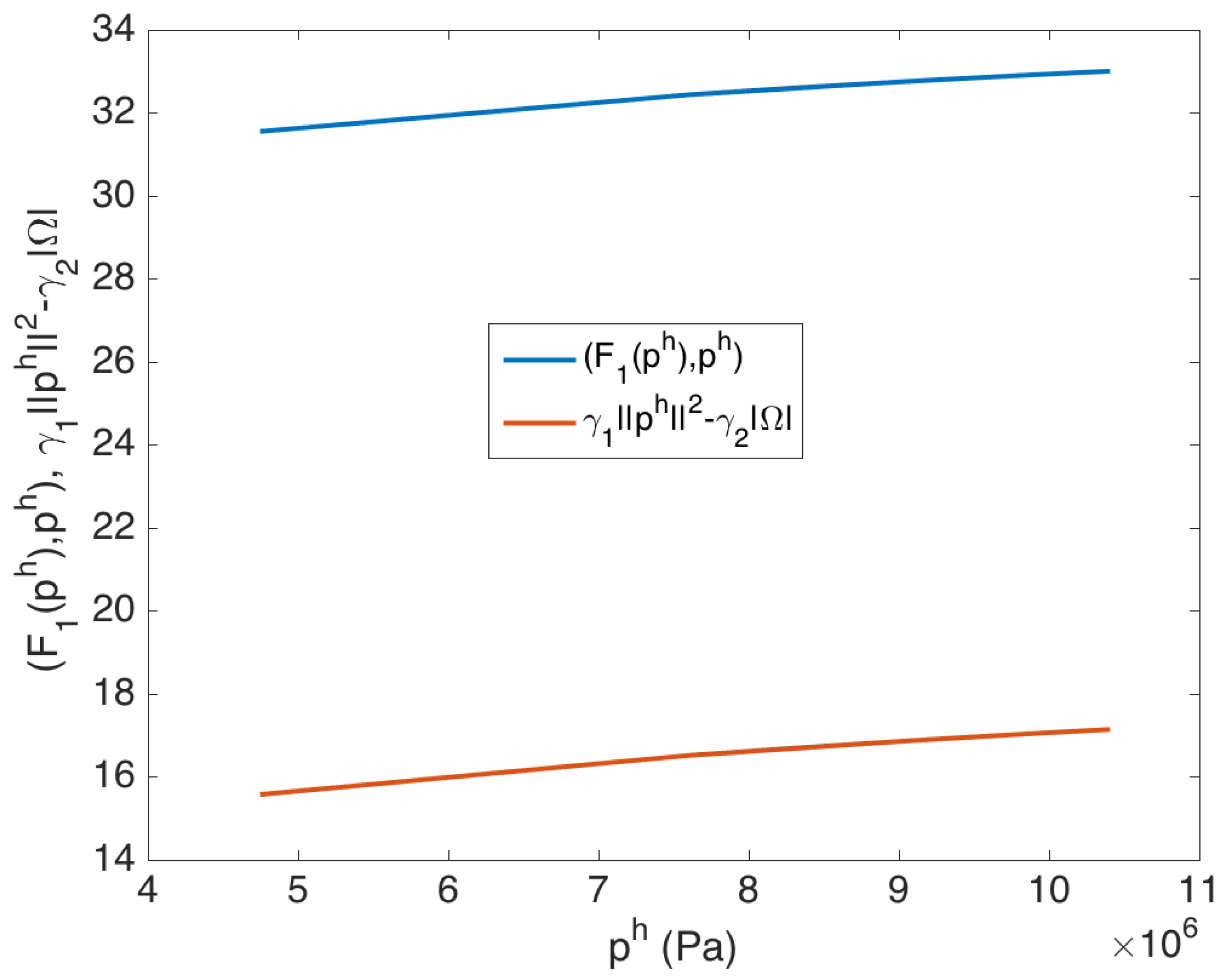
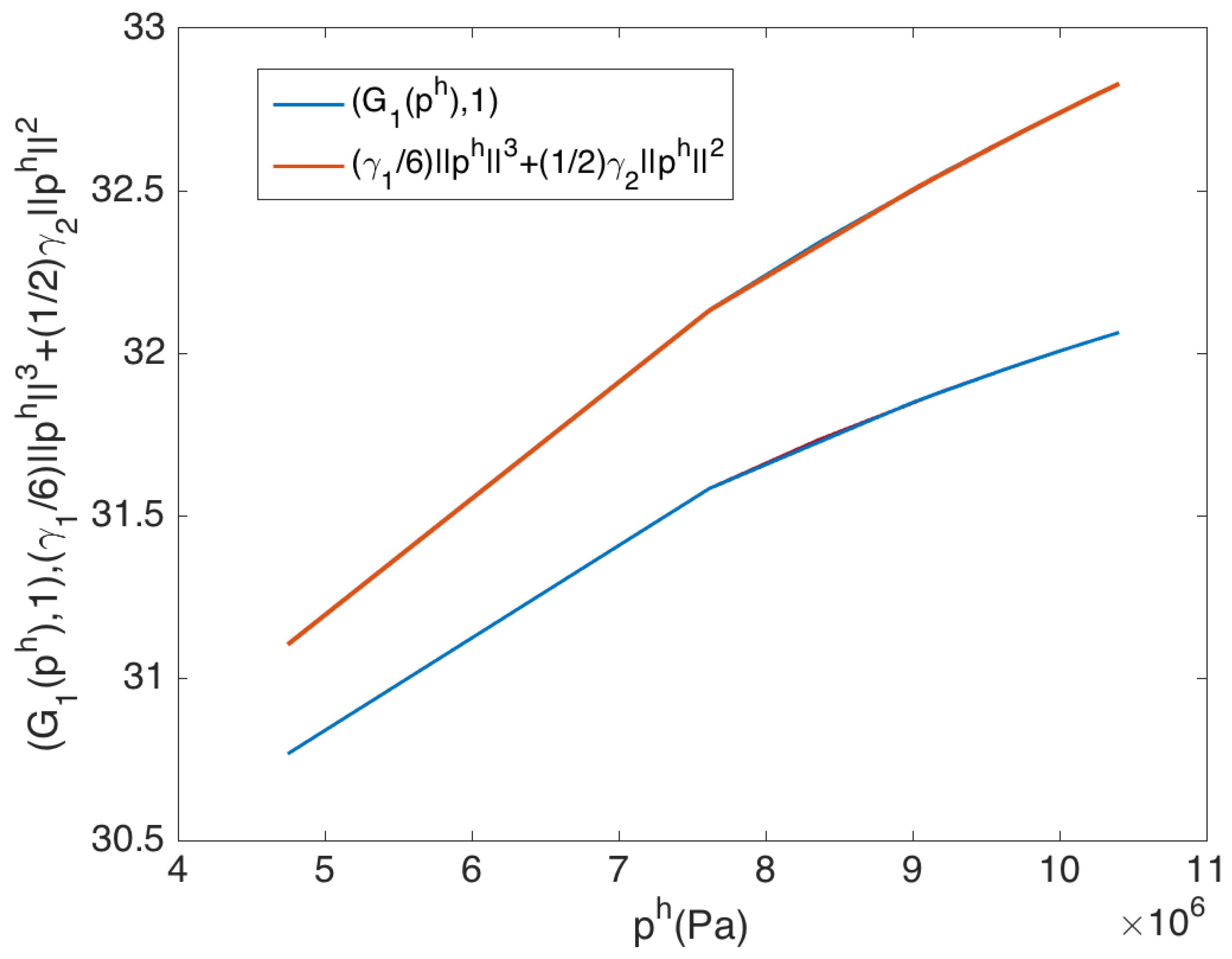
Figure 1 provides a numerical verification for the theoretical results in Lemma 1, namely, $(F_1(p^h),p^h)\ge {\gamma }_1\parallel p^h{\parallel }^2-{\gamma }_2\left|\mathsf{\Omega }\right|$. A logarithmic scale has been used in the y-axis in Figure 1. The results in Figure 1 indicates that the computed stability condition is well satisfied by the theoretical proof introduced in Lemma 1. Similarly, Figure 2 provides a numerical verification for the theoretical results in Lemma 2, namely, $(G_1(p^h),1)\le \frac{{\gamma }_1}{6}\parallel p^h{\parallel }^3+\frac{{\gamma }_2}{2}{\parallel p^h\parallel }^2.$ A logarithmic scale is used in Figure 2. Figure 2 indicates that the computed stability condition in Lemma 2 is well satisfied by the theoretical proof.

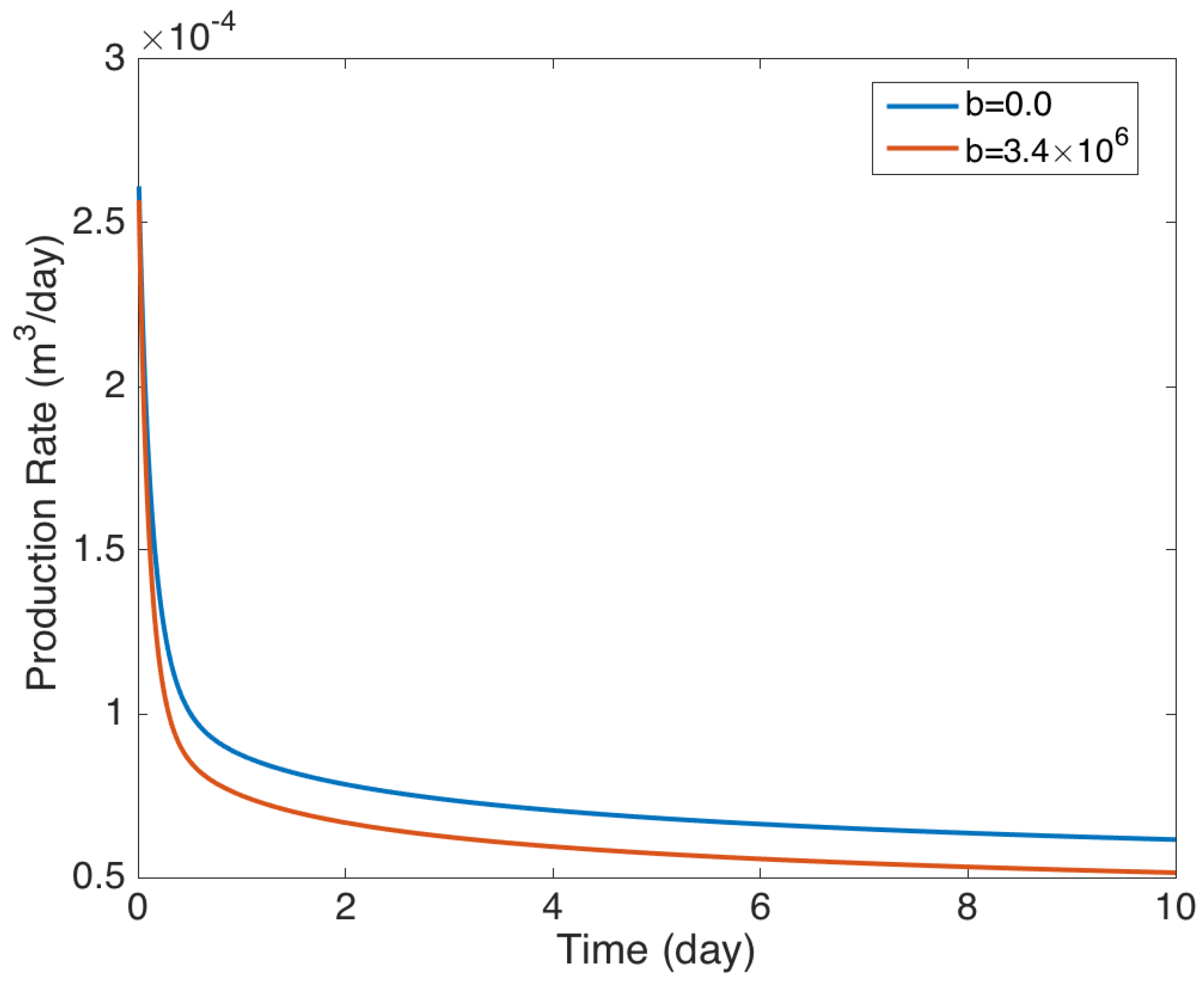
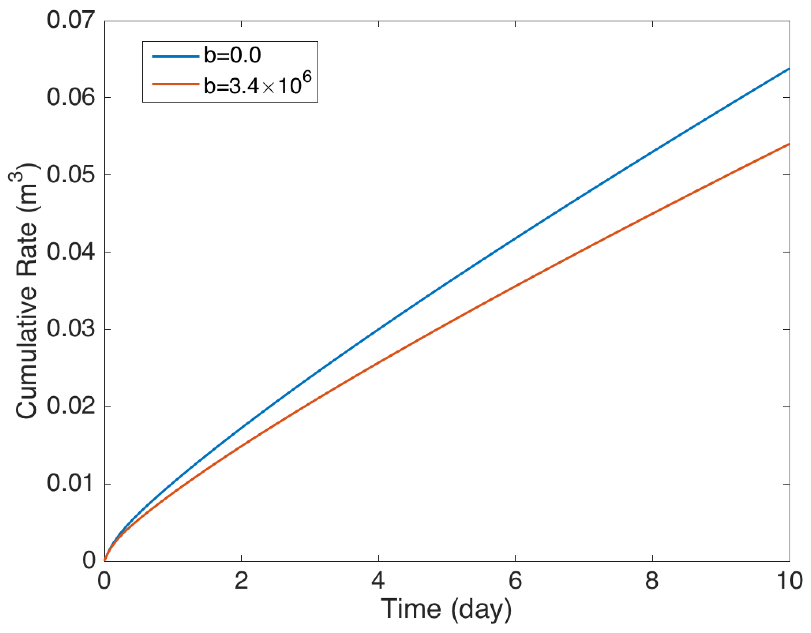
In the following, the sensitivity of the associated parameters, such as $b,\alpha$, and $\theta$, are investigated. The production rate after 10 days for various values of the slippage factor b is plotted in Figure 3. It can be seen from this figure that the slippage factor reduces the production rate. Figure 4 illustrates the cumulative production after 10 days for various values of the slippage factor b. This figure indicates clearly that the slippage factor reduces the cumulative production.

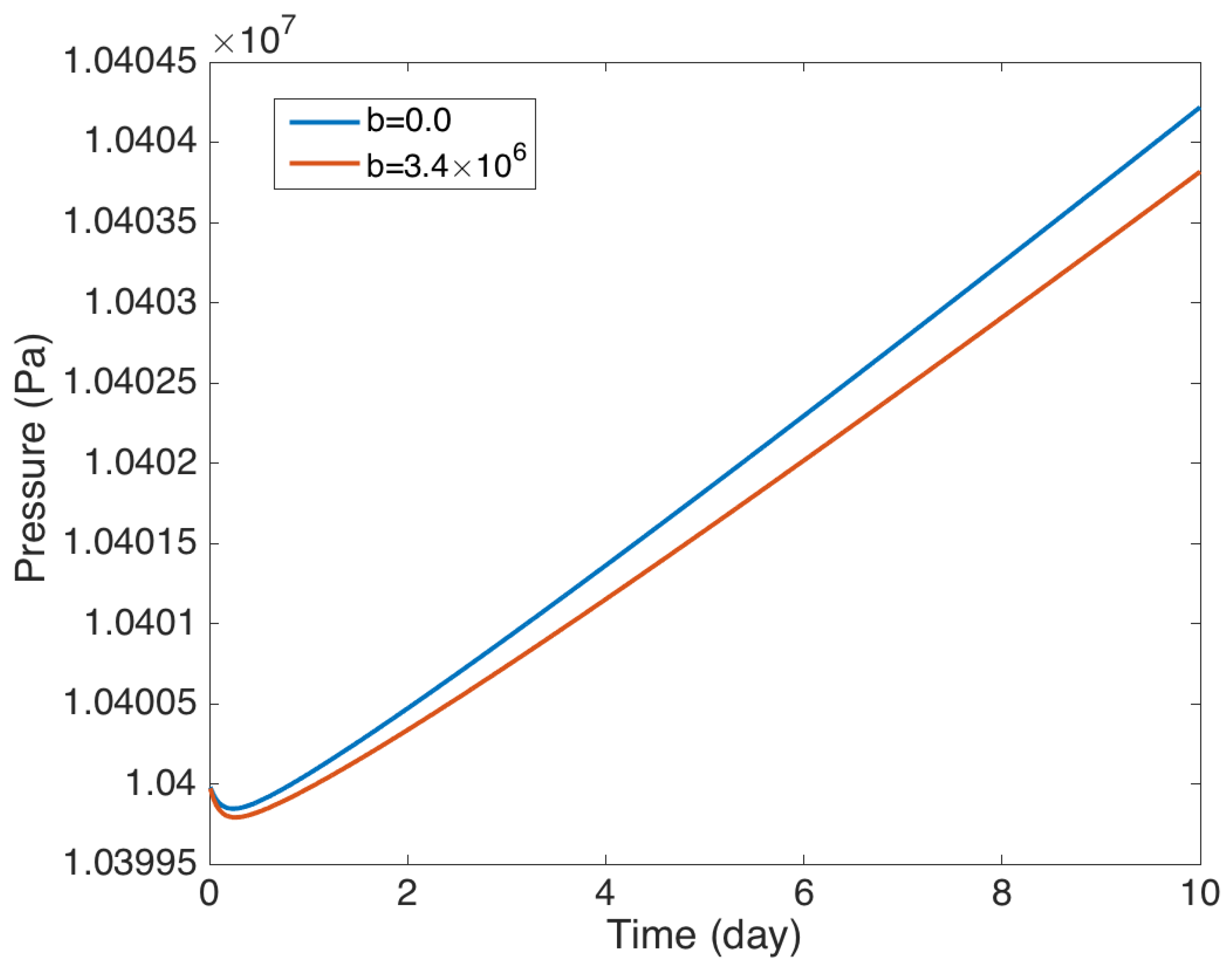
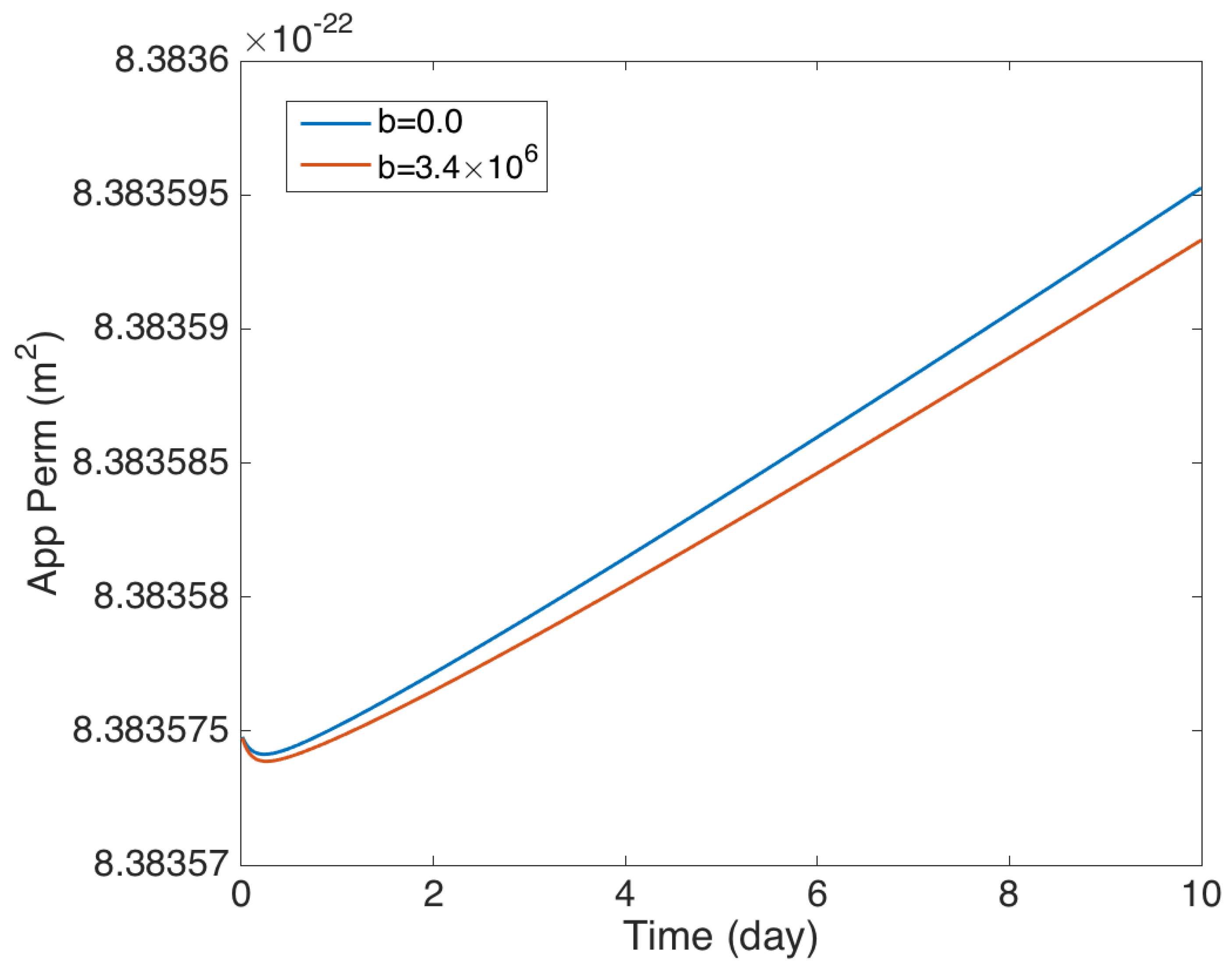
The average pressure and the average apparent permeability after 10 days of production for various values of the coefficient b are plotted, respectively, in Figure 5 and Figure 6. The two figures show a significant effect on both pressure and apparent permeability such that as coefficient b increases the pressure and the apparent permeability decrease.

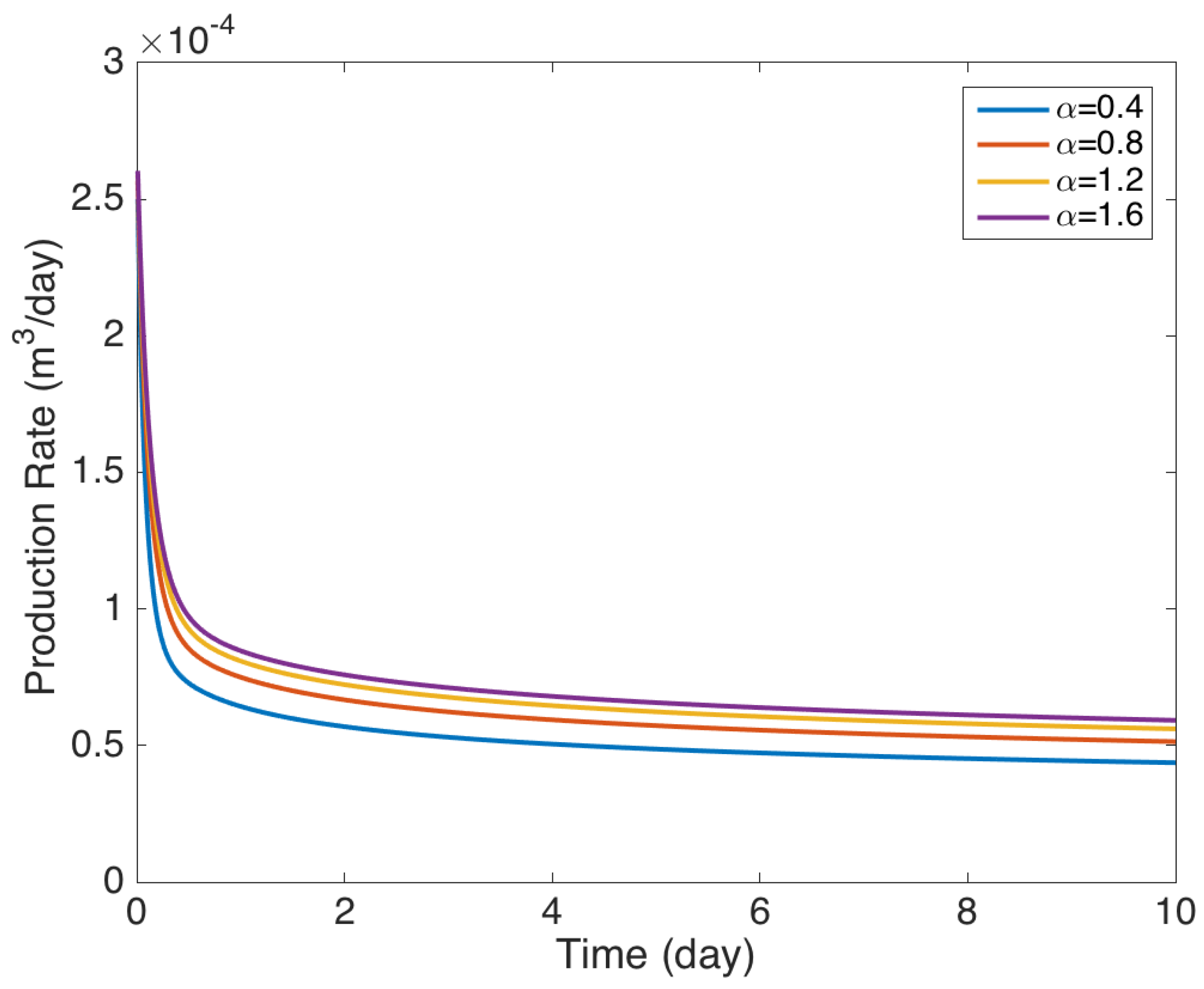
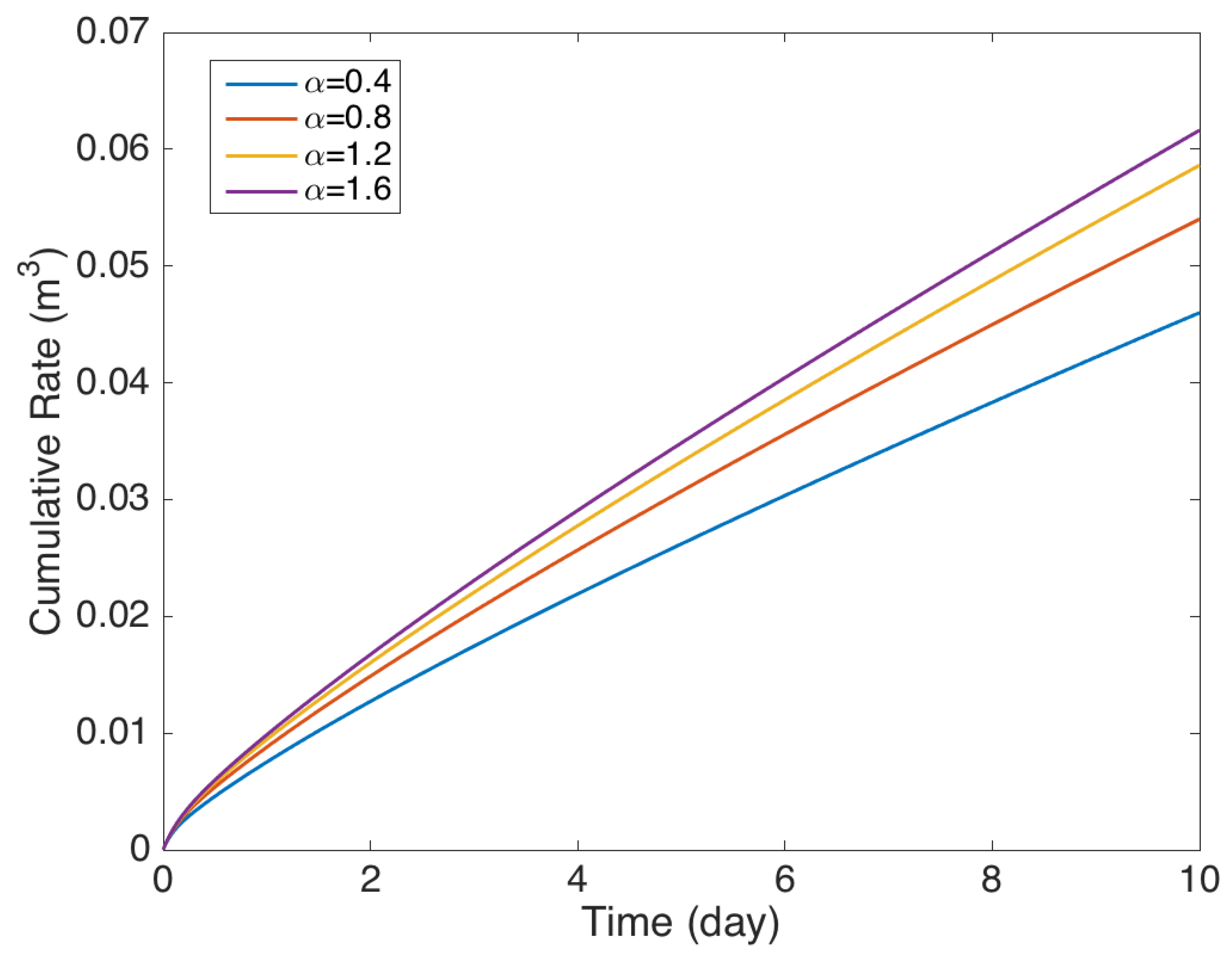
Figure 7 shows the production rate after 10 days of production for various values of the tangential momentum accommodation coefficient, $\alpha$. From this figure, one may observe that, as $\alpha$ increases, the production rate increases. Figure 8 illustrates the cumulative production after 10 days of production for various values of the tangential momentum accommodation coefficient, $\alpha$. It can be seen from this figure that, as $\alpha$ increases, the cumulative production increases.

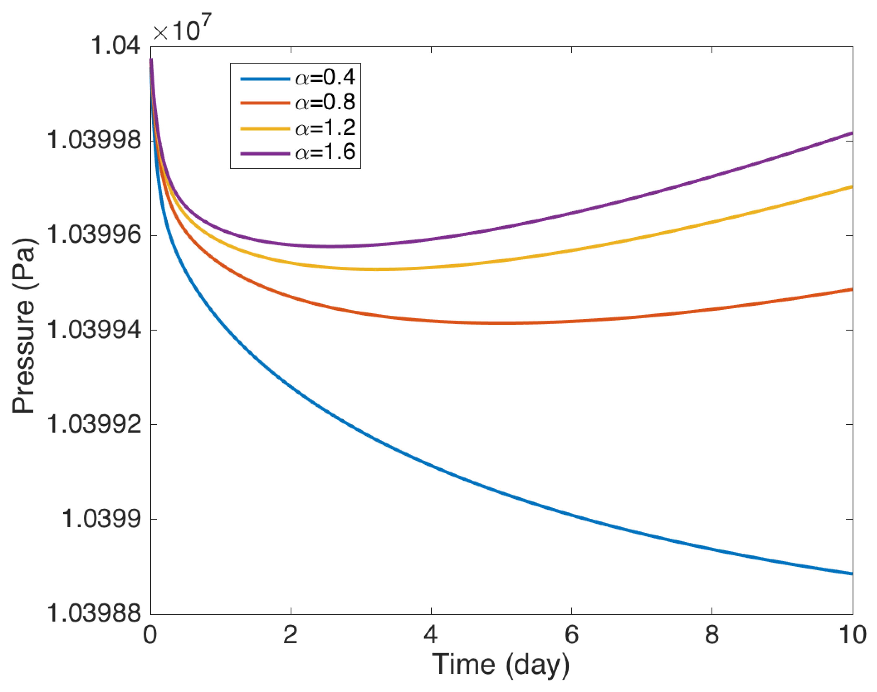
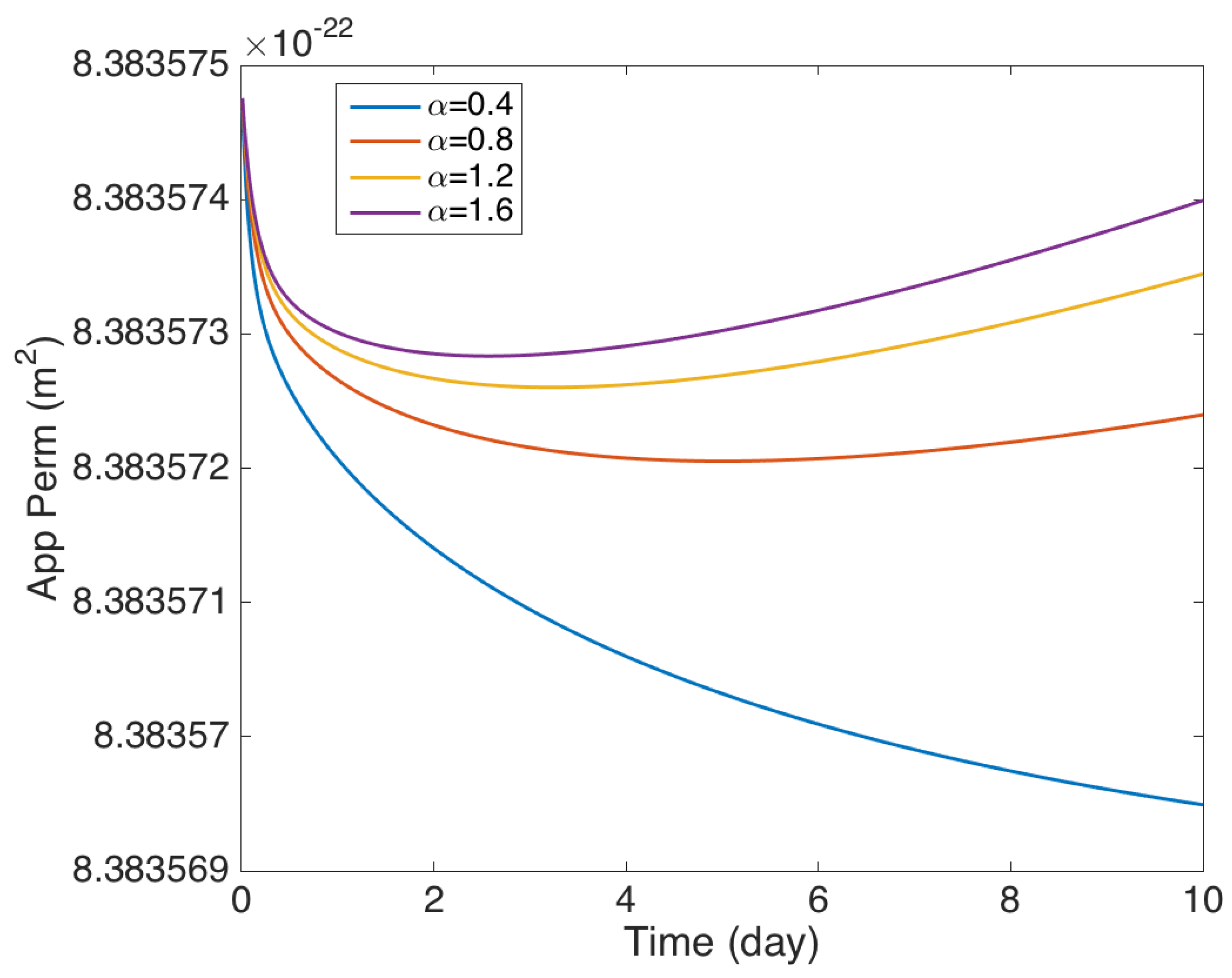
The average pressure and the average apparent permeability after 10 days for various values of the parameter $\alpha$ are plotted, respectively, in Figure 9 and Figure 10 . It is clear from these two figures that as $\alpha$ increases the pressure and the apparent permeability increase.

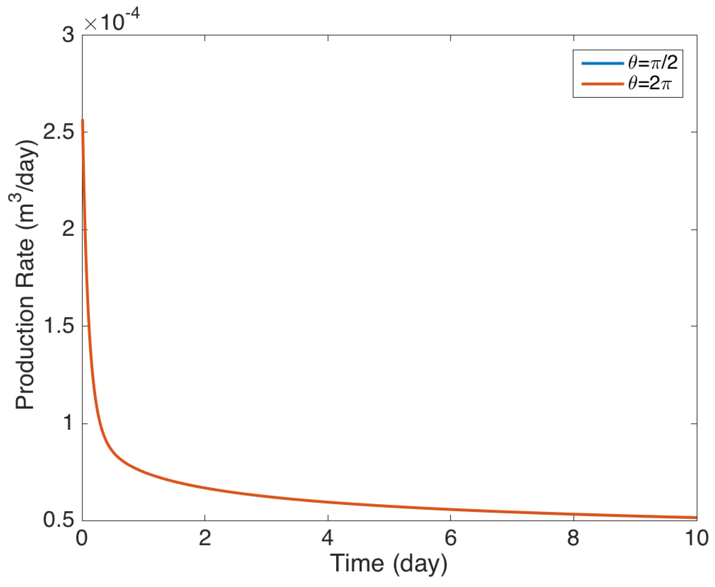
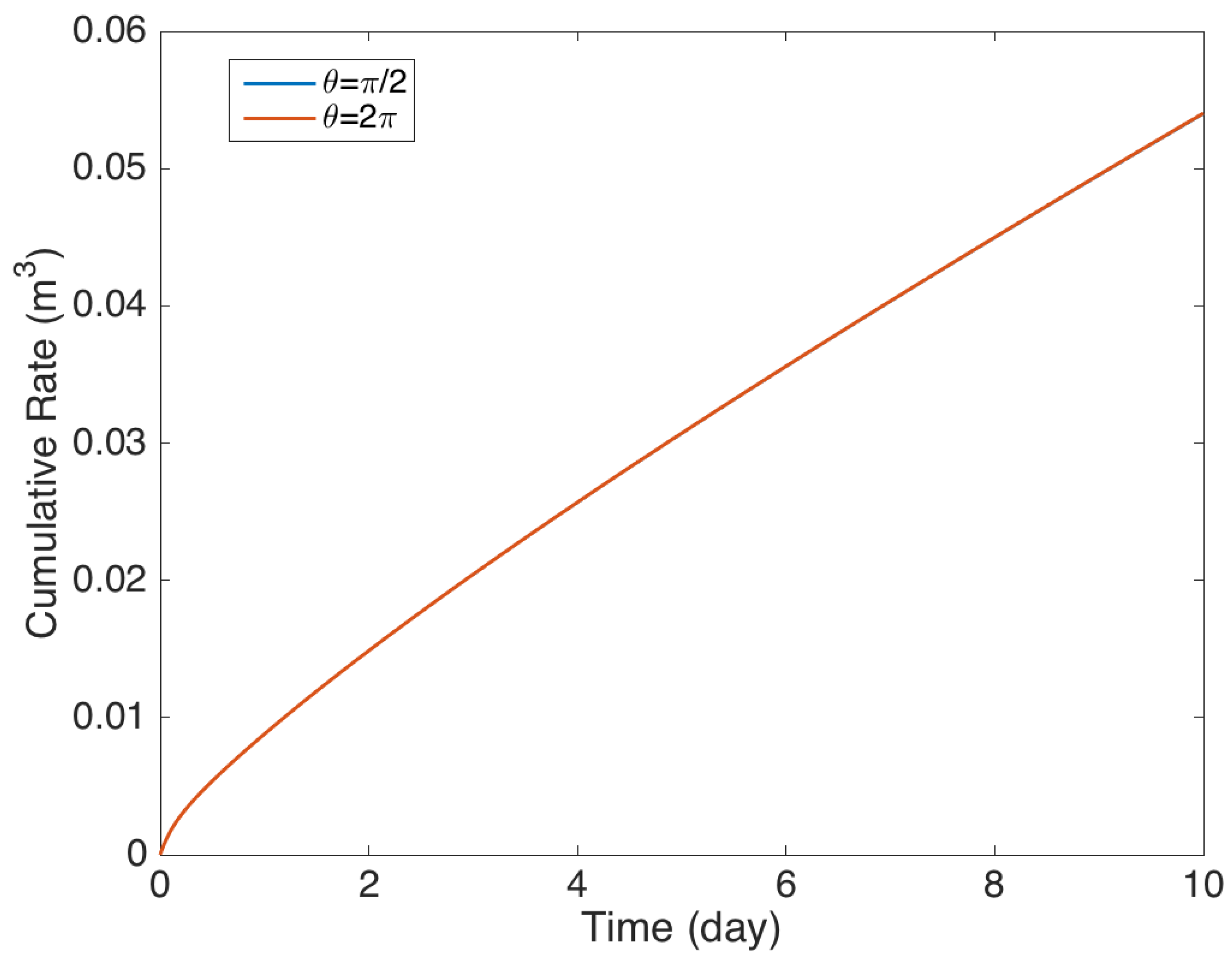
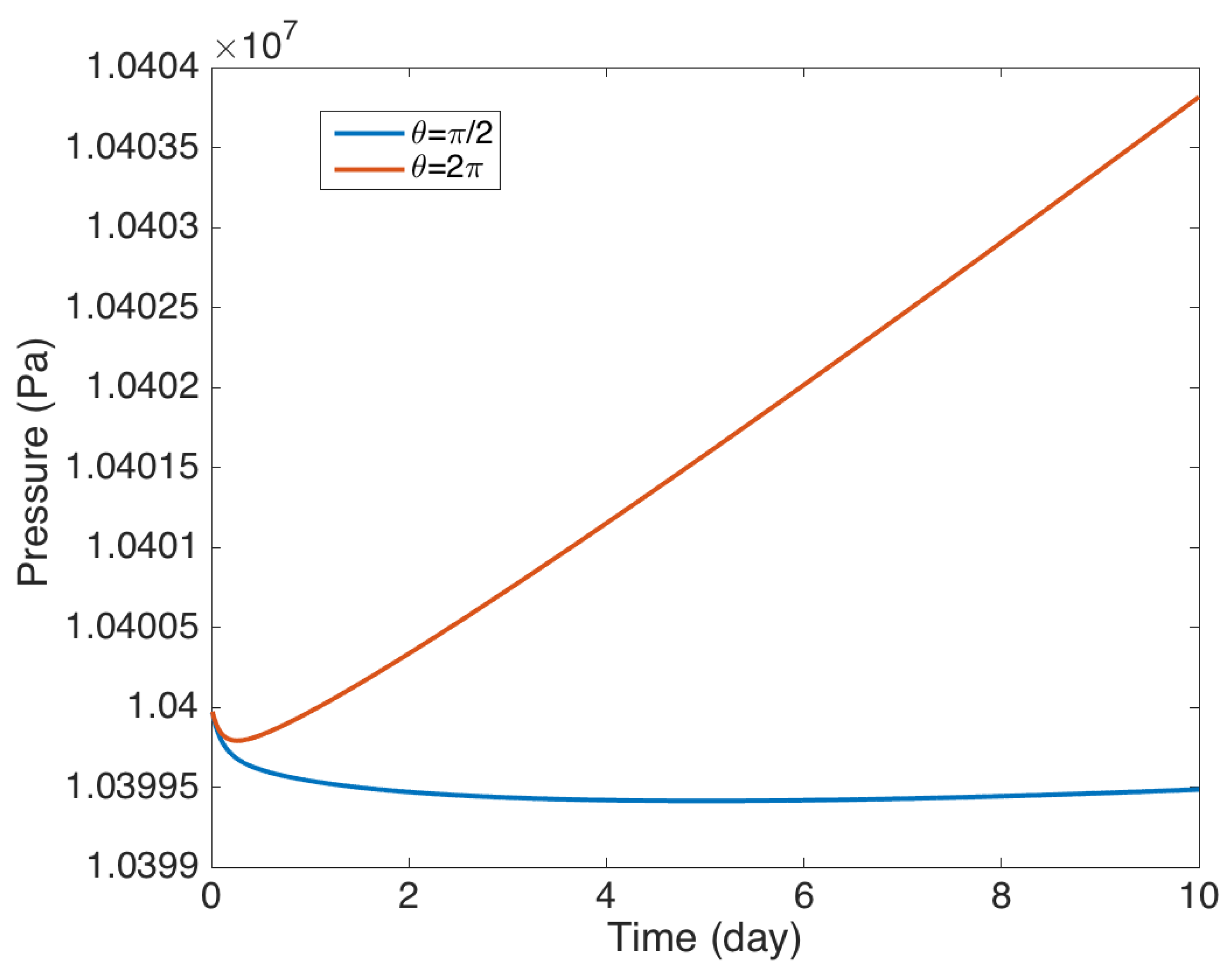
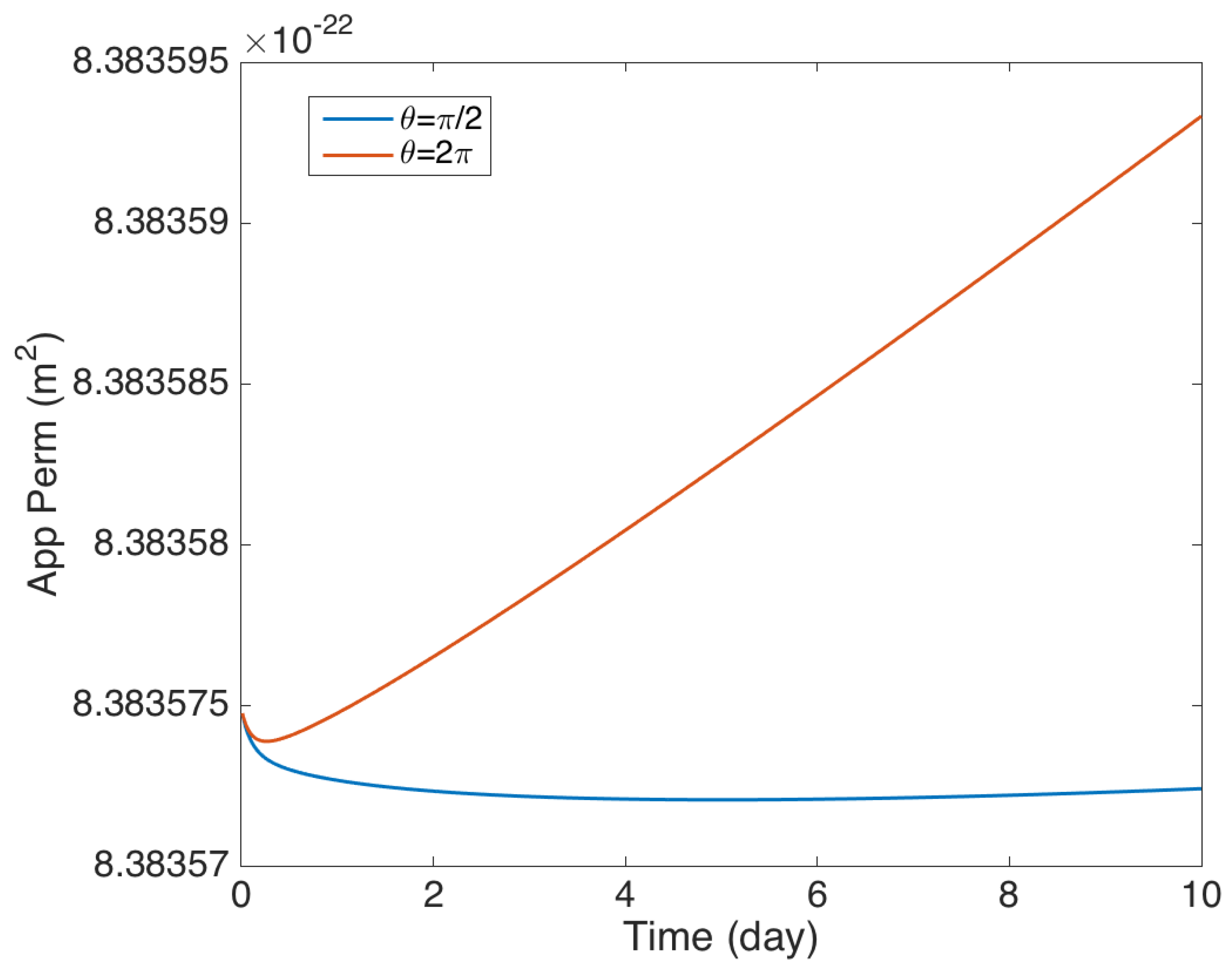
The parameter $\theta$ appears in the equation of the source of the production well, such that at $\theta =2\pi$, the production well is located in the center of the field, while, at $\theta =\frac{\pi }{2}$, the production well is located in the corner of the field. Figure 11 shows the effect of the parameter $\theta$ on the production rate after 10 days of production for $\theta =\frac{\pi }{2}$ and $\theta =2\pi$. It can be seen from this figure that when the production well is in the center, the production rate is higher. The effect of the parameter $\theta$ on the cumulative production after 10 days of production is plotted in Figure 12. This figure indicates that if the production well is located in the center, the cumulative production will be higher.

The average pressure profiles after 10 days for various values of $\theta$ are plotted in Figure 13. This figure indicates that the pressure has higher values when the production well is located in the center of the field. On the other hand, Figure 14 presents the average apparent permeability after 10 days for various values of $\theta$. It can be seen in this figure that the apparent permeability have higher values when the well is located in the center of the reservoir.

6. Conclusions

In the current paper, a mathematical model has been developed to represent the transport of the natural gas in a low permeability reservoir. The developed transport model is a single-equation contains the apparent permeability model to describe the slippage effect, and, the Langmuir isotherm model to describe the gas adsorption on the pore surface. Moreover, the Peng-Robinson equation of state has been employed to describe the thermodynamics deviation factor. On the other hand, as the MFEM is a locally conservative method, it has been used to solve the gas transport equation by splitting it into two equations, one for the pressure and the other for the velocity with two different finite element spaces. The MFEM approximates the two variables, namely, pressure and velocity, simultaneously. Additionally, a semi-implicit scheme and the backward Euler discretization have been employed for the time discretization, and the thermodynamics calculations are performed explicitly. Important compatibility conditions have been derived to guarantee the stability of the MFE algorithm, which depends on the properties of the partial differential equations. The stability analysis of the MFE algorithm has been proved in a theorem and three supported lemmas. Moreover, the stability conditions of the MFEM are verified and estimated numerically. Selected numerical experiments are performed for various values of physical parameters, the reservoir size, and the production time. Results are represented in graphs such as cumulative rate and variations in pressures and apparent permeability. One of the findings is that the apparent permeability decreases gradually as it goes away from the production well, while the opposite is true for the pressure. Variation in the apparent permeability is based on Klinkenberg effect, in which the apparent permeability depends on $1/p$. Moreover, a numerical discussion about selecting the appropriate parameters has been provided. It has been found that, as $\alpha$ increases, the production rate and the cumulative production increase. In addition, when the production well is located in the center of the field the production rate will be higher than when the production well is located in the corner. Finally, it is worth to conclude that the slippage factor b has a significant effect on the flow.

References

- Klinkenberg, L.J. The permeability of porous media to liquids and gases. In Drilling and Production Practice, American Petroleum Institute; American Petroleum Institute: Washington, DC, USA, 1941. [Google Scholar]
- McPhee, C.A.; Arthur, K.G. Klinkenberg permeability measurements: Problems and practical solutions. In Advances in Core Evaluation II: Reservoir Appraisal: Reviewed Proceedings; Edinburg Petroleum Services Ltd.: Edinburg, UK, 1991; pp. 371–392. [Google Scholar]
- Tanikawa, W.; Shimamoto, T. Comparison of Klinkenberg-corrected gas permeability and water permeability in sedimentary rocks. Int. J. Rock Mech. Min. Sci. 2009, 46, 229–238. [Google Scholar] [CrossRef]
- Wu, Y.; Pruess, K.; Persoff, P. Gas flow in porous media with Klinkenberg effects. Trans. Porous Media 1998, 32, 117–137. [Google Scholar] [CrossRef]
- Pazos, F.A.; Bhaya, A.; Compan, A.L.M. Calculation of Klinkenberg permeability, slip factor and turbulence factor of core plugs via nonlinear regression. J. Pet. Sci. Eng. 2009, 67, 159–167. [Google Scholar] [CrossRef]
- Esmaili, S.; Mohaghegh, S.D. Full field reservoir modeling of shale assets using advanced data-driven analytics. Geosci. Front. 2016, 7, 11–20. [Google Scholar] [CrossRef]
- Javadpour, F.; Fisher, D.; Unsworth, M. Nanoscale gas flow in shale gas sediments. J. Can. Pet. Technol. 2007, 46. [Google Scholar] [CrossRef]
- Javadpour, F. Nanopores and apparent permeability of gas flow in mudrocks (shales and siltstone). J. Can. Pet. Technol. 2009, 48, 16–21. [Google Scholar] [CrossRef]
- Cui, X.; Bustin, A.M.M.; Bustin, R.M. Measurements of gas permeability and diffusivity of tight reservoir rocks: different approaches and their applications. Geofluids 2009, 9, 208–223. [Google Scholar] [CrossRef]
- Shabro, V.; Torres-Verdin, C.; Javadpour, F. Numerical simulation of shale-gas production: From pore-scale modeling of slip-flow, Knudsen diffusion, and Langmuir desorption to reservoir modeling of compressible fluid. In Proceedings of the North American Unconventional Gas Conference and Exhibition, The Woodlands, TX, USA, 14–16 June 2011. [Google Scholar]
- Civan, F.; Rai, C.S.; Sondergeld, C.H. Shale-gas permeability and diffusivity inferred by improved formulation of relevant retention and transport mechanisms. Trans. Porous Media 2011, 86, 925–944. [Google Scholar] [CrossRef]
- Freeman, C.; Moridis, G.; Michael, G. Measurement, modeling, and diagnostics of flowing gas composition changes in shale gas well. In Proceedings of the Latin America and Caribbean Petroleum Engineering Conference, Mexico City, Mexico, 16–18 April 2012. [Google Scholar]
- Singh, H.; Cai, J. Screening improved recovery methods in tight-oil formations by injecting and producing through fractures. Int. J. Heat Mass Transf. 2018, 116, 977–993. [Google Scholar] [CrossRef]
- Ge, X.; Fan, Y.; Cao, Y.; Li, J.; Cai, J.; Liu, J.; Wei, S. Investigation of organic related pores in unconventional reservoir and its quantitative evaluation. Energy Fuels 2016, 30, 4699–4709. [Google Scholar] [CrossRef]
- Qi, Y.; Ju, Y.; Jia, T.; Zhu, H.; Cai, J. Nanoporous structure and gas occurrence of organic-rich shales. J. Nanosci. Nanotechnol. 2017, 17, 6942–6950. [Google Scholar] [CrossRef]
- Salama, A.; El-Amin, M.F.; Kumar, K.; Sun, S. Flow and transport in tight and shale formations. Geofluids 2017, 2017, 4251209. [Google Scholar] [CrossRef]
- El-Amin, M.F.; Amir, S.; Salama, A.; Urozayev, D.; Sun, S. Comparative study of shale-gas production using single- and dual-continuum approaches. J. Pet. Sci. Eng. 2017, 157, 894–905. [Google Scholar] [CrossRef]
- El-Amin, M.F. Analytical solution of the apparent-permeability gas-transport equation in porous media. Eur. Phys. J. 2017, 132, 129–135. [Google Scholar] [CrossRef]
- El-Amin, M.F.; Radwan, A.; Sun, S. Analytical solution for fractional derivative gas-flow equation in porous media. Res. Phys. 2017, 7, 2432–2438. [Google Scholar] [CrossRef]
- Raviart, P.A.; Thomas, J.M. A mixed finite element method for 2nd order elliptic problems, Mathematical aspects of finite element methods. Lect. Notes Math. 1977, 606, 292–315. [Google Scholar]
- Brezzi, F.; Douglas, J.; Marini, L.D. Two families of mixed finite elements for second order elliptic problems. Numer. Math. 1985, 47, 217–235. [Google Scholar] [CrossRef]
- Brezzi, F.; Fortin, V. Mixed and Hybrid Finite Element Methods; Springer: Berlin, Germany, 1991. [Google Scholar]
- Nakshatrala, K.B.; Turner, D.Z.; Hjelmstad, K.D.; Masud, A. A stabilized mixed finite element formulation for Darcy flow based on a multiscale decomposition of the solution. Comp. Meth. App. Mech. Eng. 2006, 195, 4036–4049. [Google Scholar] [CrossRef]
- El-Amin, M.F.; Kou, J.; Sun, S.; Salama, A. Adaptive time-splitting scheme for two-phase flow in heterogeneous porous media. Adv. Geo-Energy Res. 2017, 1, 182–189. [Google Scholar]
- Kou, J.; Sun, S. Unconditionally stable methods for simulating multi-component two-phase interface models with Peng-Robinson equation of state and various boundary conditions. J. Comput. Appl. Math. 2016, 291, 158–182. [Google Scholar] [CrossRef]
- Brown, G.P.; Dinardo, A.; Cheng, G.K.; Sherwood, T.K. The flow of gases in pipes at low pressures. J. Appl. Phys. 1946, 17, 802–813. [Google Scholar] [CrossRef]
- Roy, S.; Raju, R. Modeling gas flow through microchannels and nanopores. J. Appl. Phys. 2003, 93, 4870–4879. [Google Scholar] [CrossRef]
Figure 1.
Numerical verification for the theoretical results in Lemma 1.
Figure 2.
Numerical verification for the theoretical results in Lemma 2.
Figure 3.
The production rate for various values of the coefficient b.
Figure 4.
The cumulative production for various values of the coefficient b.
Figure 5.
The average pressure profiles for various values of the coefficient b.
Figure 6.
The average apparent permeability for various values of the coefficient b.
Figure 7.
The production rate for various values of .
Figure 8.
The cumulative production for various values of .
Figure 9.
The average pressure for various values of the parameter .
Figure 10.
The average apparent permeability for various values of the parameter .
Figure 11.
The production rate for various values of the parameter .
Figure 12.
The cumulative production for various values of the parameter .
Figure 13.
Figure 14.