An Analytical Flow Model for Heterogeneous Multi-Fractured Systems in Shale Gas Reservoirs

Abstract

The use of multiple hydraulically fractured horizontal wells has been proven to be an efficient and effective way to enable shale gas production. Meanwhile, analytical models represent a rapid evaluation method that has been developed to investigate the pressure-transient behaviors in shale gas reservoirs. Furthermore, fractal-anomalous diffusion, which describes a sub-diffusion process by a non-linear relationship with time and cannot be represented by Darcy’s law, has been noticed in heterogeneous porous media. In order to describe the pressure-transient behaviors in shale gas reservoirs more accurately, an improved analytical model based on the fractal-anomalous diffusion is established. Various diffusions in the shale matrix, pressure-dependent permeability, fractal geometry features, and anomalous diffusion in the stimulated reservoir volume region are considered. Type curves of pressure and pressure derivatives are plotted, and the effects of anomalous diffusion and mass fractal dimension are investigated in a sensitivity analysis. The impact of anomalous diffusion is recognized as two opposite aspects in the early linear flow regime and after that period, when it changes from 1 to 0.75. The smaller mass fractal dimension, which changes from 2 to 1.8, results in more pressure and a drop in the pressure derivative.

1. Introduction

The development of shale gas in North America has achieved large-scale commercial success [1,2,3], which has set off a shale gas revolution worldwide. As a key technology in shale gas exploration and development, well testing plays an irreplaceable role. The characteristics of shale gas reservoirs can be obtained through the transient pressure analysis of multiple fractured horizontal wells (MFHWs) in shale gas reservoirs.

In order to describe the random and complex fractures, some works [4,5] have investigated discrete fracture networks through numerical simulation approaches. Tang et al. [4] established a three-dimensional numerical model based on the construction of spatial discretization by the finite volume method. Wang [5] proposed a unified model for shale gas reservoirs based on discrete fracture networks to investigate shale gas production by rate transient analysis. However, this requires numerical simulation, and the process is time-consuming and occupies a large amount of computing resources.

Fortunately, the analytical approach is a convenient and rapid method for the evaluation of dynamic characteristics of the shale gas reservoir, which takes less time and needs less reservoir data compared with numerical simulation approaches. Thus, the analytical approach has been used in more applications in recent years.

Two types of analytical model are used to analyze transient pressure behaviors. One type is the detailed analytical model, which is based on the source function and superposition principle [6,7,8]. This characterizes the stimulated reservoir volume (SRV) region in a shale gas reservoir as a circular or rectangular zone and extends the one-region model to a dual-region composite model. Similarly, the shortcomings of the detailed analytical model also cause a large increase in the amount of calculation required. In order to describe the SRV region more concisely and conveniently, the other type, which is linear models, such as the tri-linear flow model [9] and the five-region flow model [10], was developed. The five-region flow model was established based on the tri-linear flow model and takes into account not only the stimulated region, but also the nearby unstimulated region. These two models represent a rapid way to capture key characteristics in shale gas reservoirs.

Based on these two analytical models (the detailed analytical model and linear model), other improved models were developed, e.g., models considering the effects of fractures in the SRV region [11], non-equal spacing fractures [12], fracture networks in the shale matrix [13,14], the non-Darcy high-speed flow inside the hydraulic fracture [15], the shale matrix diffusion and dual porosity model [16], a transient flow approach [17], and non-Darcy flow with a threshold pressure gradient in tight gas reservoirs [18]. Recently, Zeng et al. [19], Zeng [20], and Zeng et al. [21] proposed a seven-region flow model, which takes into account the spatial heterogeneity and typical seepage features, such as ad-desorption and diffusion in shale gas reservoirs. Unfortunately, all of the models described above only consider the linear flow in all regions, and thereby neglect the fractal features and sub-diffusive flow in the SRV region.

In order to capture the features of fractal geometry and sub-diffusive flow in highly heterogeneous porous media, an analytical flow model that considers anomalous diffusion and other significant features to describe the flow characteristics in the SRV region has been proposed [22,23,24,25,26].

Chen and Raghavan [22] utilized fractional derivatives to characterize the process of anomalous diffusion in the complex fractures and took into account the continuous-time random walk in hydraulically fractured reservoirs with single porosity. Subsequently, Ren and Guo [23] presented a dual porosity and anomalous diffusion model for shale gas reservoirs. Unfortunately, they did not consider the heterogeneity of multi-fractured systems by applying a three-region or five-region model. Later, Albinali and Ozkan [24] proposed a tri-linear anomalous diffusion and dual-porosity model that uses fractional calculus to account for non-uniform velocity in porous media. However, the fractal geometry features of the induced fractures in the SRV region are not considered in the model. Wang et al. [25] considered the fractal characteristics in the complex system by coupling fractal relations to account for the heterogeneity in the SRV region. Fan and Ettehadtavakkol [26] applied micro-seismic data to verify the fractal flow model and proposed a semi-analytical model for rate transient analysis in shale gas reservoirs.

All the models described above do not fully consider the various diffusion of shale gas in the shale matrix, the dual porosity in the SRV region, or the stress sensitivity of permeability and fractal-anomalous diffusion in complex fractures.

Table 1. Feature comparisons of analytical models for multiple fractured horizontal wells (MFHWs). SRV: stimulated reservoir volume.

Serial Number	Features	Models
		Stalgorova and Mattar [10]	Albinali and Ozkan [24]	Wang et al. [25]	Fan and Ettehadtavakkol [26]	Present Model
1	Fractal permeability in SRV	-	-	Fractal	Tortuosity-dependent	Fractal
2	Dual porous media in SRV	Cubic geometry	Spherical geometry	Cubic geometry	Slab geometry	Spherical geometry
3	Diffusion in fractures	Normal	Anomalous	Normal	Normal	Anomalous
4	Pressure-dependence of permeability	-	-	-	-	Exponential
5	Slip flow in shale matrix	-	-	-	Klinkenberg	Klinkenberg
6	Diffusion in shale matrix	-	-	-	Knudsen	Composite
7	Ad-desorption	-	-	-	Langmuir	Langmuir
8	Flow types	Five regions	Three regions	Five regions	Three regions	Five regions

demonstrates the differences by comparing previous analytical flow models with the present model. Previous models only considered homogeneous properties and simple transport mechanisms in shale gas reservoirs.

Based on the above, this work proposes a new analytical model based on fractal-anomalous diffusion. Firstly, the present model is coupled with anomalous diffusion and other significant features, such as ad-desorption, slip flow, surface flow, pressure-dependent permeability, and fractal geology. Using the Laplace transformation method and Duhamel’s theorem [27], the analytical solution of the present model is obtained. Then, the flow regimes are identified, and the effects of relevant parameters are analyzed.

Therefore, the present model can effectively describe the complex fracture networks in the SRV region and more accurately account for the various transport mechanisms of MFHWs in shale gas reservoirs. Due to the lack of well-testing data in shale gas reservoirs, the present model has only been applied to one case, but more cases will be studied in the future.

2. Physical Model

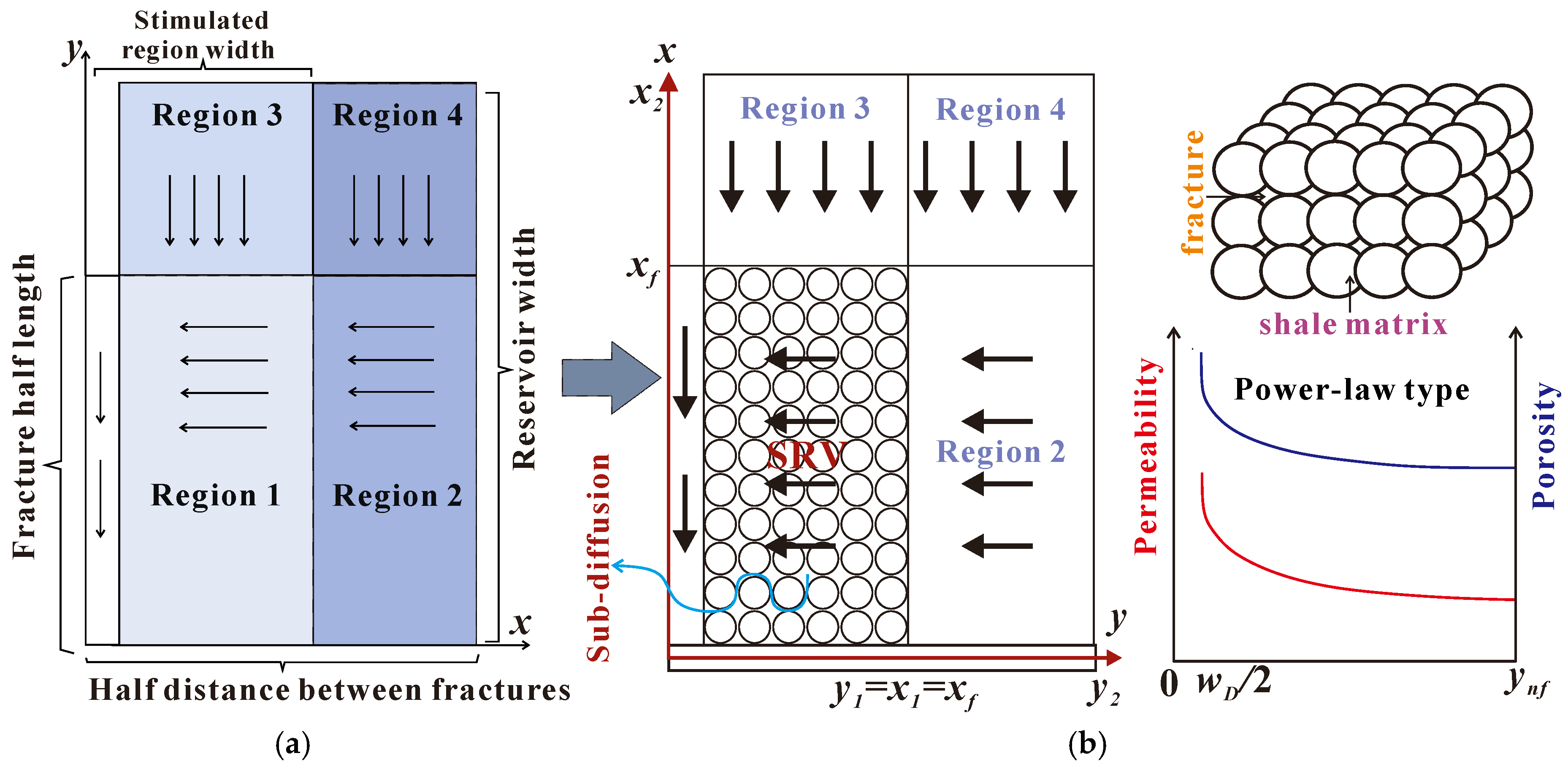
Figure 1 is a schematic of the typical five-region flow model and the improved five-region flow model (new model) in a shale gas reservoir. Higher fractal permeability, dual-porosity, and anomalous diffusion in the SRV region are taken into account around each fracture. The other three regions occupy the remaining space between adjacent fractures. One-quarter of each hydraulic fracture is taken into account due to the assumption of symmetry in the reservoir.

As shown in Figure 1, the reservoir between two adjacent fractures is subdivided into five regions in the improved five-region flow model. There is vertical linear flow from region 4 to region 2 and from region 3 to region 1 (SRV). Similarly, horizontal linear flow exists from region 2 to region 1 and from region 1 to each hydraulic fracture. Compared with the typical five-region flow model, ad-desorption and various diffusion in the shale matrix, dual-porosity (shown as spherical matrix in Figure 1), the fractal geometry (shown as a power-law type in Figure 1) and anomalous diffusion (sub-diffusion) in the SRV region, and stress-sensitive permeability in each region are considered in this work. The main assumptions of this new model are as follows:

(1)

A hydraulically fractured horizontal well is at the center of a closed shale gas reservoir;

(2)

Each hydraulic fracture is perpendicular to the horizontal well, spaced uniformly along the horizontal wellbore, and has the same length;

(3)

Fluid flow in each region is a one-dimensional single-phase flow;

(4)

Desorption in shale matrix yields to the Langmuir isotherm adsorption law;

(5)

The continuity of flux and pressure at interfaces is used to couple the adjacent regions.

3. Mathematical Model

3.1. Mechanisms and Properties

3.1.1. Adsorption/Desorption and Apparent Permeability

Shale gas adsorption in the shale matrix typically yields to the Langmuir isotherm adsorption law, and pseudo-pressure can be written as follows [28,29]:

$$V_E=V_L\frac{P}{P_L+P}$$

(1)

where V_E is defined as the adsorption equilibrium concentration (sm³/m³), the Langmuir adsorption concentration is represented by V_L (sm³/m³), the Langmuir pressure is represented by $P_L$ (MPa), and P means the pressure in the reservoir (MPa).

$${\sigma }_m=1+\frac{{\rho }_{gsc}{V}_L{p}_L}{c_g{\rho }_m{\varphi }_m{\left(p_L+p\right)}^2}$$

(2)

where ${\sigma }_m$ is the adsorption factor.

$$m\left(p\right)=2\underset{p_0}{\overset{p}{{\displaystyle \int }}}\frac{p}{\mu {\rm Z}}dp$$

(3)

where m(p) is the pseudo-pressure (MPa²/(mPa·s)), the gas viscosity is represented by μ (mPa·s), and the real gas deviation factor is represented by z.

The main transport mechanisms in the shale matrix are surface diffusion, Knudsen diffusion, and slip flow. Based on the results of previous research, the expression of total equivalent permeability (apparent permeability) is as follows [30]:

$$k_{ma}=k_e+k_d+k_s={\beta }_t{k}_{ins}$$

(4)

where k_ma is defined as an apparent permeability which is related to surface diffusion, Knudsen diffusion, and slip flow (m²); k_e is the equivalent slip rate of slip flow (m²); the Knudsen diffusion equivalent permeability is represented by k_d (m²); the surface diffusion equivalent permeability is represented by k_s (m²); and ${\beta }_t$ is the matrix comprehensive diffusion factor that considers the slip flow, Knudsen, and surface diffusion.

3.1.2. Fractal Permeability and Porosity in Induced Fractures

The distribution of induced fractures is extremely complex and irregular, and therefore, it is not accurate enough to describe the porosity of induced fractures in Euclidean geometry. Fractal geometry has been verified as an effective method to describe the complex pore structure of fibrous porous media [31,32,33,34]. Based on fractal geometry, fractal permeability and fractal porosity in induced fractures comply with a power-law type as follows [35,36,37,38]:

$$K_f\left(r\right)=K_{fr}{\left(\frac{r}{L_{ref}}\right)}^{d_f-d_e-\theta }$$

(5)

where K_fr is the permeability at the reference length, $L_{ref}$ is the reference length; the mass fractal dimension of the inducec fractures is represented by $d_f$, the Euclidean dimension is represented by $d_e$, the radial coordinate value at any point is represented by r, and the tortuosity index is represented by θ.

$${\varnothing }_f\left(r\right)={\varnothing }_{fr}{\left(\frac{r}{L_{ref}}\right)}^{d_f-d_e}$$

(6)

where $\varnothing$_fr is the porosity at the reference length.

3.1.3. Anomalous Diffusion in Induced Fractures

In induced fractures, the disorder, non-local, and memory features should be considered in the SRV region. This complex transport process is anomalous diffusion, which is described by fractional calculus. The modified Darcy flow velocity is given by the following form [22]:

$$\upsilon \left(r,t\right)=-\frac{k_{\alpha }}{\mu }\frac{{\partial }_{1-\propto }}{\partial t}\nabla p\left(r,t\right).$$

(7)

The fractional derivative $\frac{{\partial }^{\propto }f\left(t\right)}{\partial t^{\propto }}$ is defined as follows [39]:

$$\frac{{\partial }^{\propto }f\left(t\right)}{\partial t^{\propto }}=\frac{1}{\Gamma \left(1-\alpha \right)}{{\displaystyle \int }}_0^t{\left(t-t^{\prime }\right)}^{-\alpha }\frac{\partial f\left(t^{\prime }\right)}{\partial t^{\prime }}d{t}^{\prime }$$

(8)

where the Gamma function is represented by $\Gamma \left(x\right)$. The Laplace transform of the fractional derivative $\frac{{\partial }^{\propto }f\left(t\right)}{\partial t^{\propto }}$ is

$${{\displaystyle \int }}_0^{\infty }{e}^{-st}\frac{{\partial }^{\propto }f\left(t\right)}{\partial t^{\propto }}dt=s^{\alpha }f\left(s\right)-s^{\alpha -1}f\left(0\right).$$

(9)

when $\alpha =1$, Equation (7) is reduced to the classical Darcy’s law as follows [23]:

$$\upsilon \left(r,t\right)=-\frac{k_{\alpha }}{\mu }\nabla p\left(r,t\right).$$

(10)

3.1.4. Pressure-Dependent Permeability

The permeability in hydraulically fracturing shale gas reservoirs is sensitive to pore pressure, according to previous experiments [3,40]. Given the relationship with pore pressure, fractal permeability is introduced by permeability modulus as follows:

$$k=k_i{e}^{-\gamma \left(m_i-m\right)}$$

(11)

where k_i is the permeability under the initial pseudo-pressure ($m_i$), the corresponding pseudo-pressure in the reservoir is represented by $m$, and $\gamma$ is the stress sensitivity factor.

3.2. Governing Flow Equations and Solutions

In order to obtain the final solution, the governing diffusivity equations for each region are written with the relevant initial and boundary conditions. Definitions of all dimensionless terms are given in Appendix A.

3.2.1. Unstimulated Regions (Region 4 + Region 3 + Region 2)

Starting with the fourth region, the diffusivity equation that considers the ad-desorption and various diffusion can be written in a dimensionless form:

$$e^{-{\gamma }_D^{*}{m}_{4D}}[\frac{{\partial }^2{m}_{4D}}{\partial x_D^2}-{\gamma }_D^{*}{(\frac{\partial m_{4D}}{\partial x_D^2})}^2]=\frac{{\sigma }_m}{{\beta }_t{\eta }_{4D}}\frac{\partial m_{4D}}{\partial t_D}$$

(12)

where ${\gamma }_D^{*}$ is the dimensionless stress-sensitive factor.

The perturbation inversion proposed by Pedrosa Jr. [41] is applied to pseudo-pressure, as presented in Equation (13).

$$m_D=-\frac{1}{{\gamma }_D^{*}}ln\left(1-{\gamma }_D^{*}{\phi }_D\left(r_D,t_D\right)\right)$$

(13)

Additionally, a zero-order approximation is performed to linearize the diffusivity equation. Then, the diffusion Equation (12) can be approximately written in a Laplace form, as follows:

$$\frac{{\partial }^2{\overline{\phi }}_{4D}}{\partial x_D^2}=\frac{{\sigma }_{m}s}{{\beta }_t{\eta }_{4D}}{\overline{\phi }}_{4D}.$$

(14)

The outer boundary condition (no-flow) is

$$\frac{\partial {\overline{\phi }}_{4D}}{\partial x_D}{|}_{x_D=x_{eD}}=0.$$

(15)

The inner boundary condition (pressure continuity) is

$${\overline{\phi }}_{4D}{|}_{x_D=x_{nfD}=1}={\overline{\phi }}_{2D}{|}_{x_D=x_{nfD}=1}.$$

(16)

Therefore, the general form of the solution in the fourth region can be given as follows:

$${\overline{\phi }}_{4D}={\overline{\phi }}_{2D}{|}_{x_D=x_{nfD}=1}\frac{cosh\left[\sqrt{f_4\left(s\right)}\left(x_D-x_{eD}\right)\right]}{cosh\left[\sqrt{f_4\left(s\right)}\left(x_{nfD}-x_{eD}\right)\right]}{|}_{x_{nfD}=1}$$

(17)

where

$$f_4\left(s\right)=\frac{{\sigma }_{m}s}{{\beta }_t{\eta }_{4D}}$$

(18)

and ${\eta }_{4D}$ is the dimensionless conductivity in region 4.

Region 3, which has low permeability, can only flow vertically to region 1. Similarly, a general form of the solution for the third region can be given as follows:

$${\overline{\phi }}_{3D}={\overline{\phi }}_{1D}{|}_{x_D=x_{nfD}=1}\frac{cosh\left[\sqrt{f_3\left(s\right)}\left(x_D-x_{eD}\right)\right]}{cosh\left[\sqrt{f_3\left(s\right)}\left(x_{nfD}-x_{eD}\right)\right]}{|}_{x_{nfD}=1}$$

(19)

where

$$f_3\left(s\right)=\frac{{\sigma }_{m}s}{{\beta }_t{\eta }_{3D}}.$$

(20)

Also, the governing equation of region 2 becomes

$$\frac{{\partial }^2{\overline{\phi }}_{2D}}{\partial y_D^2}=\frac{{\sigma }_{m}s}{{\beta }_t{\eta }_{2D}}{\overline{\phi }}_{2D}-\frac{k_{4a}}{k_{2a}{x}_{nfD}}\frac{\partial {\overline{\phi }}_{4D}}{\partial {\mathrm{x}}_D}{|}_{{\mathrm{x}}_D=x_{nfD}=1}.$$

(21)

The outer boundary condition (no-flow) is

$$\frac{\partial {\overline{\phi }}_{2D}}{\partial y_D}{|}_{y=y_{eD}}=0.$$

(22)

The inner boundary condition (pressure continuity) is

$${\overline{\phi }}_{2D}{|}_{y_D=y_{nfD}}={\overline{\phi }}_{nfD}{|}_{y_D=y_{nfD}}.$$

(23)

Therefore, the solution for region 2 becomes

$${\overline{\phi }}_{2D}={\overline{\phi }}_{nfD}{|}_{y_D=y_{nfD}}\frac{cosh\left[\sqrt{f_2\left(s\right)}\left(y_D-y_{eD}\right)\right]}{cosh\left[\sqrt{f_2\left(s\right)}\left(y_{nfD}-y_{eD}\right)\right]}$$

(24)

where

$$f_2\left(s\right)=\frac{{\sigma }_{m}s}{{\beta }_t{\eta }_{2D}}-\frac{k_{4a}}{k_{2a}{x}_{nfD}}\sqrt{f_4\left(s\right)}tanh\left[\sqrt{f_4\left(s\right)}\left(x_{nfD}-x_{eD}\right)\right]{|}_{x_{nfD}=1}.$$

(25)

3.2.2. Region 1 (SRV)

Region 1 represents the SRV region in which the transient inter-porosity flow from the matrix to fracture subsystem is applied. Moreover, the anomalous diffusion, fractal permeability, and porosity in induced fractures are also considered.

- Matrix subsystem:

Similarly, the pressure solution in the matrix subsystem of region 1 can be obtained:

$${\overline{\phi }}_{1mD}=\frac{sinh\left(\sqrt{u_{1m}\left(s\right)}{r}_{mD}\right)}{r_{mD}sinh\left(\sqrt{u_{1m}\left(s\right)}\right)}{\overline{\phi }}_{nfD}$$

(26)

where

$$u_{1m}\left(s\right)=\frac{15\left(1-{\omega }_1\right){\sigma }_{m}s}{{\beta }_t{\lambda }_1{\eta }_{1D}}.$$

(27)

- Induced fractures subsystem:

The diffusivity equation of the complex fractures networks can be derived in the following dimensionless form. More detailed derivations are given in Appendix B.

$$\frac{{\partial }^2{\overline{\phi }}_{nfD}}{\partial y_D^2}+\frac{d_f-\theta -2}{y_D}\frac{\partial {\overline{\phi }}_{nfD}}{\partial y_D}=f_1\left(s\right)y_D{}^{\theta }{\overline{\phi }}_{nfD}$$

(28)

where

$$f_1\left(s\right)=\frac{{\omega }_1}{{\eta }_{1D}}{s}^{\alpha }+\left\{\frac{{\beta }_t{\lambda }_1}{5}[\sqrt{u_{1m}(s)}coth(\sqrt{u_{1m}(s)}-1)]-{\left(\frac{{\eta }_{nf}}{x_f^2}\right)}^{\alpha -1}\frac{k_{3a}}{k_{nf}}\sqrt{f_3\left(s\right)}tanh[\sqrt{f_3\left(s\right)}\left(x_{nfD}-x_{eD}\right)]\right\}{s}^{\alpha -1}$$

(29)

The outer boundary condition (flow continuity) is

$$k_{2a}\frac{\partial {\overline{\phi }}_{2fD}}{\partial y_D}{|}_{y_D=y_{nfD}=}{\left(s\frac{{\eta }_{nf}}{x_f^2}\right)}^{1-\alpha }{k}_{nf}{y}_D{}^{d_f-\theta -2}\frac{\partial {\overline{\phi }}_{nfD}}{\partial y_D}{|}_{y_D=y_{nfD}}.$$

(30)

The inner boundary condition (pressure continuity) is

$${\overline{\phi }}_{nfD}{|}_{y_D=w_D/2}={\overline{\phi }}_{FD}{|}_{y_D=w_D/2}.$$

(31)

Therefore, the general form of the pressure solution in the SRV is

$${\overline{\phi }}_{nfD}=y_D{}^a\left\{A{I}_n\left[\alpha y_D{}^{\frac{1}{\alpha }}\sqrt{f_1\left(s\right)}\right]+B{K}_n\left[\alpha y_D{}^{\frac{1}{\alpha }}\sqrt{f_1\left(s\right)}\right]\right\}$$

(32)

where

$$\{\begin{array}{c}a=\frac{1-b}{2},b=d_f-\theta -2,n=\frac{1-b}{2+\theta },\alpha =\frac{2}{2+\theta },c=\alpha \sqrt{f_1\left(s\right)}\\ A=\frac{h_{22}{\overline{\phi }}_{FD}{|}_{y_D=w_D/2}}{h_{11}{h}_{22}-h_{12}{h}_{21}},B=\frac{-h_{21}{\overline{\phi }}_{FD}{|}_{y_D=w_D/2}}{h_{11}{h}_{22}-h_{12}{h}_{21}}\\ h_{11}={\left(\frac{w_D}{2}\right)}^a{I}_n[c{\left(\frac{w_D}{2}\right)}^{\frac{1}{\alpha }}]\\ h_{12}={\left(\frac{w_D}{2}\right)}^a{K}_n[c{\left(\frac{w_D}{2}\right)}^{\frac{1}{\alpha }}]\\ h_{21}=g{\left(y_{nfD}\right)}^a\sqrt{f_2\left(s\right)}tanh\left[\left(y_{nfD}-y_{eD}\right)\sqrt{f_2\left(s\right)}\right]I_n\left[c{\left(y_{nfD}\right)}^{\frac{1}{\alpha }}\right]-\frac{c}{\alpha }{\left(y_{nfD}\right)}^{a+\frac{1}{\alpha }-1}{I}_{n-1}[c{\left(y_{nfD}\right)}^{\frac{1}{\alpha }}]\\ h_{22}=g{\left(y_{nfD}\right)}^a\sqrt{f_2\left(s\right)}tanh\left[\left(y_{nfD}-y_{eD}\right)\sqrt{f_2\left(s\right)}\right]K_n\left[c{\left(y_{nfD}\right)}^{\frac{1}{\alpha }}\right]+\frac{c}{\alpha }{\left(y_{nfD}\right)}^{a+\frac{1}{\alpha }-1}{K}_{n-1}[c{\left(y_{nfD}\right)}^{\frac{1}{\alpha }}]\end{array}$$

(33)

3.2.3. Hydraulic Fracture Region

Considering that the stress sensitivity of permeability and flow exchange is directly related to the quality dimension, the diffusivity equation in hydraulic fractures becomes

$$e^{-{\gamma }_D^{*}{m}_{FD}}[\frac{{\partial }^2{m}_{FD}}{\partial x_D^2}-{\gamma }_D^{*}{\left(\frac{\partial m_{FD}}{\partial x_D^2}\right)}^2]=\frac{1}{{\eta }_{FD}}\frac{\partial m_{FD}}{\partial t_D}-\frac{2}{F_{CD}}{(\frac{w_D}{2})}^{-\theta }{\left(s\frac{{\eta }_{nf}}{x_f^2}\right)}^{1-\alpha }\frac{\partial m_{nfD}}{\partial y_D}{|}_{y_D=\frac{w_D}{2}}$$

(34)

where

$$F_{CD}=\frac{k_F{w}_D}{k_{nf}}.$$

(35)

The perturbation inversion [41] and zero order approximation in the Laplace form are applied, and the diffusivity equation then becomes

$$\frac{{\partial }^2{\overline{\phi }}_{FD}}{\partial x_D^2}=\frac{s}{{\eta }_{FD}}{\overline{\phi }}_{FD}-\frac{2}{F_{CD}}{(\frac{w_D}{2})}^{-\theta }{\left(s\frac{{\eta }_{nf}}{x_f^2}\right)}^{1-\alpha }\frac{\partial {\overline{\phi }}_{nfD}}{\partial y_D}{|}_{y_D=\frac{w_D}{2}}.$$

(36)

Equation (35) can be written as follows:

$$\frac{{\partial }^2{\overline{\phi }}_{FD}}{\partial x_D^2}=F\left(s\right){\overline{\phi }}_{FD}$$

(37)

where

$$\{\begin{array}{c}F\left(s\right)=\frac{s}{{\eta }_{FD}}-\frac{2}{F_{CD}}{\left(\frac{w_D}{2}\right)}^{-\theta }{\left(s\frac{{\eta }_{nf}}{x_f^2}\right)}^{1-\alpha }\frac{\partial {\overline{\phi }}_{nfD}}{\partial y_D}{|}_{y_D=\frac{w_D}{2}}\\ \frac{\partial {\overline{\phi }}_{nfD}}{\partial y_D}{|}_{y_D=\frac{w_D}{2}}=\frac{c}{\alpha }{(\frac{w_D}{2})}^{a+\frac{1}{\alpha }-1}\left\{A{I}_{n-1}\left[c{\left(\frac{w_D}{2}\right)}^{\frac{1}{\alpha }}\right]-B{K}_{n-1}\left[c{\left(\frac{w_D}{2}\right)}^{\frac{1}{\alpha }}\right]\right\}\end{array}.$$

(38)

Boundary condition 1 is

$$\frac{\partial {\overline{\phi }}_{FD}}{\partial x_D}{|}_{x_D=1}=0_{.}$$

(39)

Boundary condition 2 is

$$\frac{\partial {\overline{\phi }}_{FD}}{\partial x_D}{|}_{x_D=0}=-\frac{\pi }{F_{CD}s}.$$

(40)

The pressure solution for the hydraulic fracture region is

$${\overline{\phi }}_{FD}=\frac{\pi }{F_{CD}s}\frac{1}{\sqrt{F\left(s\right)}}\frac{cosh\left[\sqrt{F\left(s\right)}\left(x_D-x_{nfD}\right)\right]}{sinh\left[\sqrt{F\left(s\right)}{x}_{nfD}\right]}{|}_{x_{nfD}=1}.$$

(41)

Thus, the pressure solution at the wellbore can be given as follows:

$${\overline{\phi }}_{wD}={\overline{\phi }}_{FD}\left(0\right)=\frac{\pi }{F_{CD}s\sqrt{F\left(s\right)}tanh\left[x_{nfD}\sqrt{F\left(s\right)}\right]}{|}_{x_{nfD}=1}.$$

(42)

However, by applying the superposition principle and Duhamel’s principle [27], the final solution for wellbore pressure considering convergence and storage is written as follows:

$${\overline{\phi }}_{wD}\left(s_c,c_D\right)=\frac{s{\overline{\phi }}_{wD}+s_c}{s\left[1+c_{D}s\left(s{\overline{\phi }}_{wD}+s_c\right)\right]}.$$

(43)

Then, the perturbation inversion [41] and Stehfest numerical inversion [42] are applied. Finally, the pressure solution at the downhole can be written with the real-time data as

$$m_{wD}=-\frac{ln\left[1-{\gamma }_D^{*}\right]L^{-1}\left({\overline{\phi }}_{wD}\right)}{{\gamma }_D^{*}}.$$

(44)

4. Discussion and Analysis

4.1. Flow Regimes

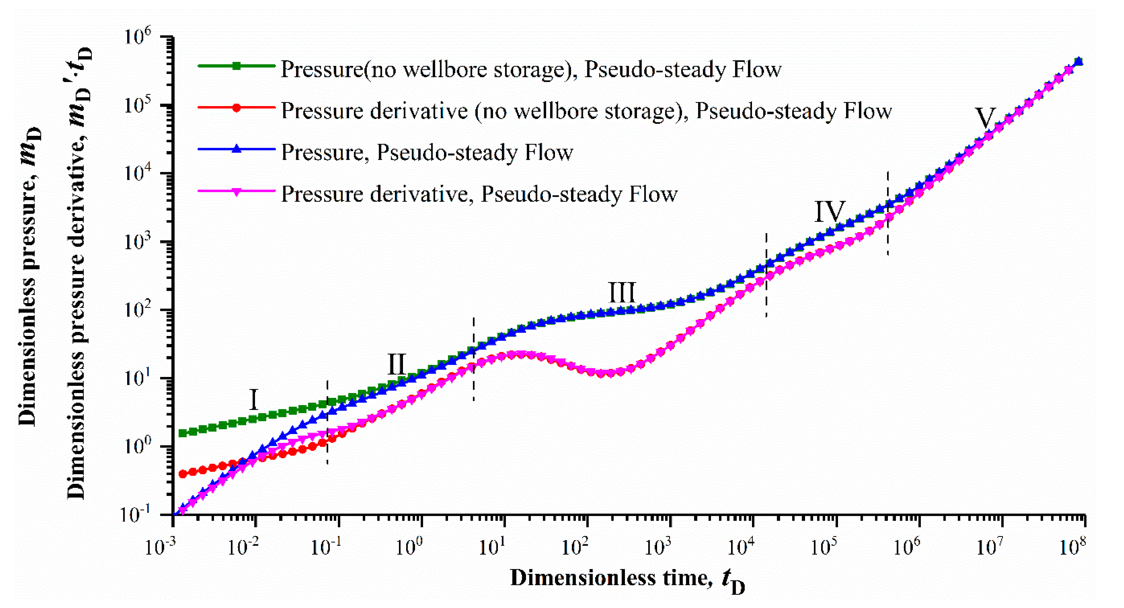
In order to obtain the main flow regimes of the improved five-region flow model, the type curves of the pressure-transient response were plotted by employing pseudo-steady inter-porosity flow in the SRV region.

The related parameters are listed in Table 1. Figure 2 shows the pressure-transient response of MFHWs in shale gas reservoirs. There are five flow stages on the type curves: (1) bilinear flow in each hydraulic fracture and in the SRV region (region 1), where the pressure derivative curve’s slope is 1/4 (α = 1, and d_f = 2); (2) first linear flow in the SRV region, where the pressure derivative curve shows a straight line with a slope of 1/2 (α = 1, and d_f = 2); (3) inter-porosity and fractal-anomalous diffusion in the SRV region; (4) second linear flow from the USRV to SRV region, where the pseudo-pressure derivative curve presents a straight line with a slope of 1/2 (α = 1, and d_f = 2); and (5) pseudo-steady flow (boundary control flow), where the pseudo-pressure and pseudo-pressure derivative curves are all represented by straight lines with a unit slope.

4.2. Sensitivity Analysis

In the corresponding sensitivity analysis, firstly, one relevant parameter was changed while keeping the other parameters at their original values. Then, all the relevant parameters were changed at the same time. Model parameters were given values in the simulation by referring to relevant literature [6,12,16,17,23,25,26], and they are listed in

Table 2. Model parameters.

Parameter Name	Parameter Value
Dimensionless half fracture length, xfD	1
Dimensionless fracture conductivity, FCD	2
Inter-porosity flow coefficient, λ	λ = 0.2
Storage capacity coefficient, ω	ω = 0.2
Dimensionless distance in x direction, xnfD/xeD	xnfD = 1, xeD = 50
Dimensionless distance in y direction, ynfD/yeD	ynfD = 1, yeD = 50
Ratio of permeability, ki/kj	k3a/knf = 0.0005, k2a/knf = 0.1, k4a/k2a = 0.02
Absorption factor, ${\sigma }_m$	5
Diffusion factor (apparent permeability coefficient), βt	1.1
Dimensionless stress sensitivity factor, ${\gamma }_D^{*}$	0.00009
Anomalous diffusion exponent, α	0.85
Tortuosity index, θ	0.35
Mass fractal dimension, df	1.9
Number of fractures, n	10

.

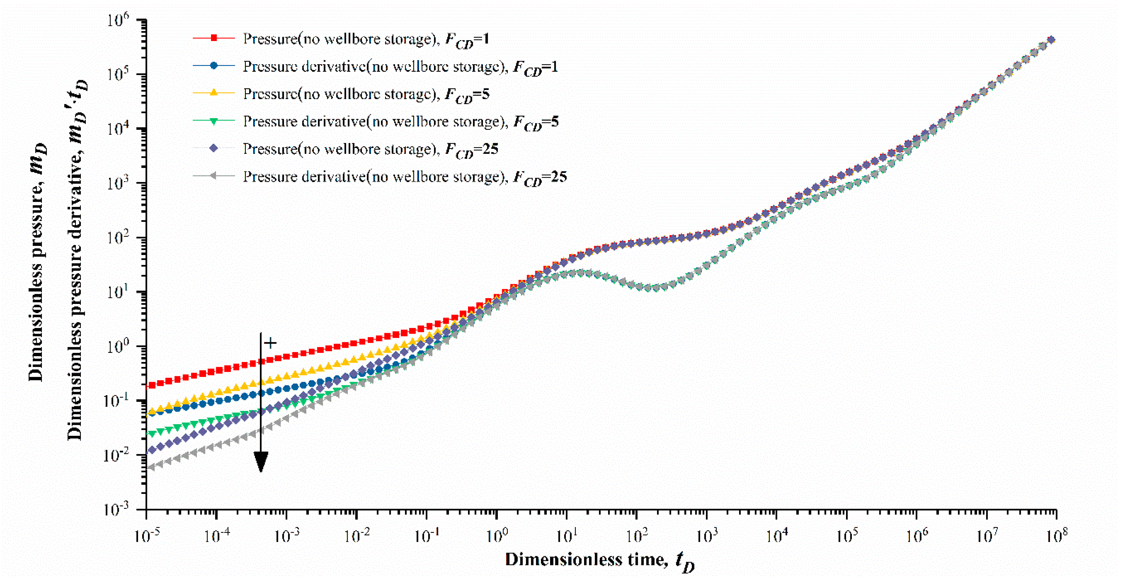
Figure 3 shows that the fracture conductivity mainly affects the early flow stages. The greater the fracture conductivity is, the smaller the gas flow resistance is, and the smaller pressure consumption is with the same production. It is not difficult to see that the fracture conductivity mainly influences the pressure and pressure derivative curves in the bilinear flow and first linear flow stages. With an increase in the fracture conductivity, the duration of the bilinear flow stage decreases and the duration of the first linear flow stage increases. As seen in Figure 3, when F_CD = 25, only the first linear flow regime can be observed.

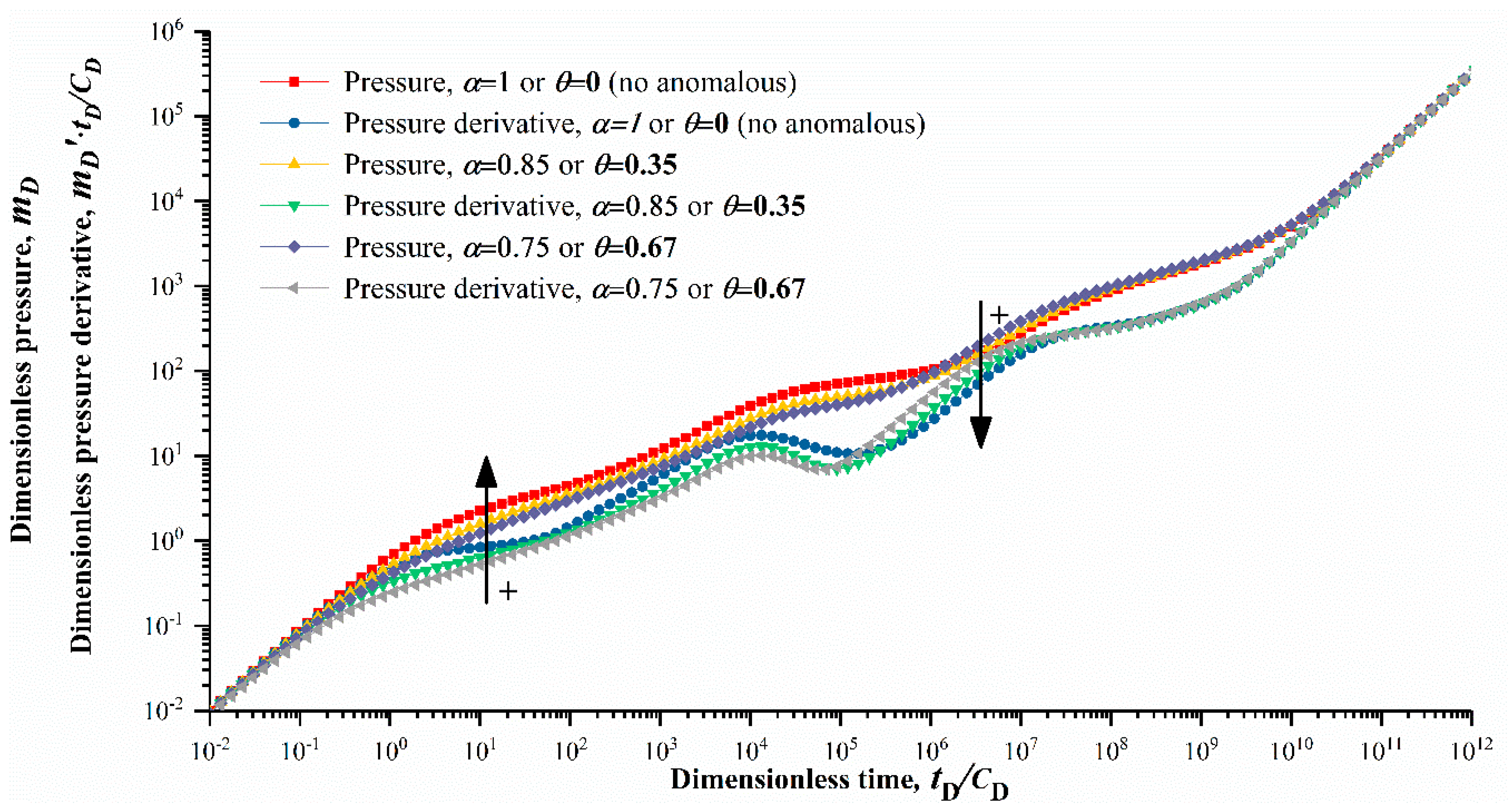
Figure 4 demonstrates the type curves of the pressure and pressure derivative for MFHWs in a shale gas reservoir with various anomalous diffusion exponent (α) and tortuosity index (θ) values. As can be seen, one intersection point exists between the anomalous diffusion and classical diffusion pressure derivative curves. At the early bilinear and linear flow stages, the pressure and pressure derivative for α < 1 or θ > 0 (anomalous diffusion) are smaller than those for α = 1 or θ = 0 (classical diffusion). When the value of α increases (θ decreases), the pressure and its derivative will also increase. The reason for this is that anomalous diffusion delays the performance of pressure derivative behaviors. However, after the inter-porosity flow stage, with different α values, the difference will be more obvious, and the trend is the opposite. In other words, a decrease in α (θ increasing) causes the pressure and its derivative to increase over time. This accounts for the characteristic of sub-diffusion (slower flow) when α < 1 or θ > 0 (anomalous diffusion).

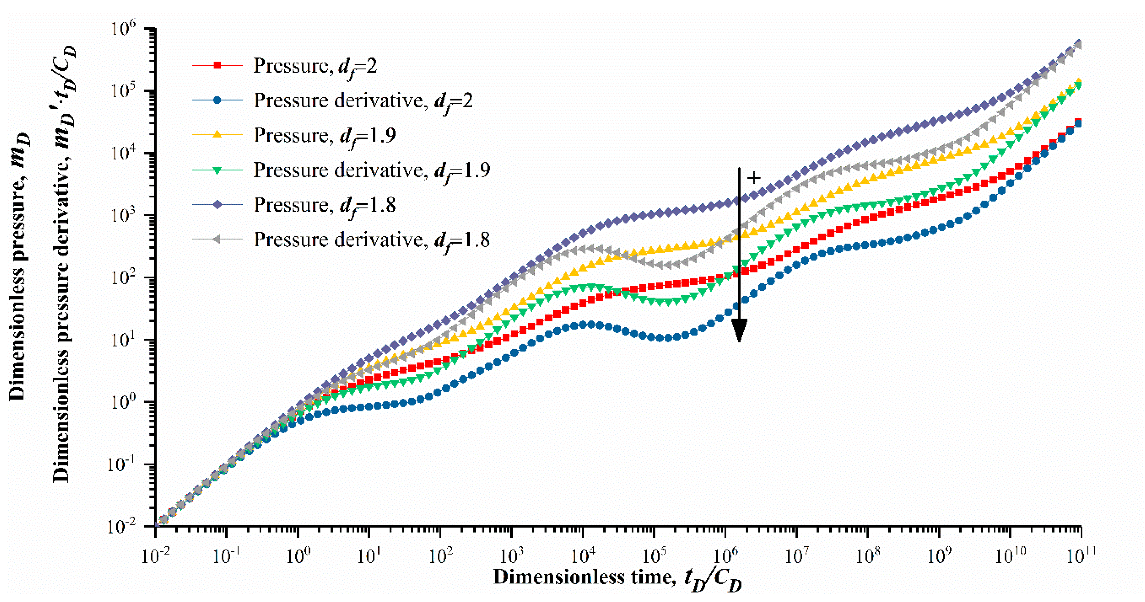
Figure 5 shows that the mass fractal dimension of induced fractures (Hausdorff index) has a significant effect on the pressure behavior at almost all the stages, except for the wellbore storage stage. Overall, the smaller the mass fractal dimension is, the larger the gas flow resistance is and the greater the pressure consumption is with the same production. As can be seen, the locations of the type curves are higher with a smaller d_f. The reason for this is that a smaller d_f value represents more resistance in the complex induced fractures.

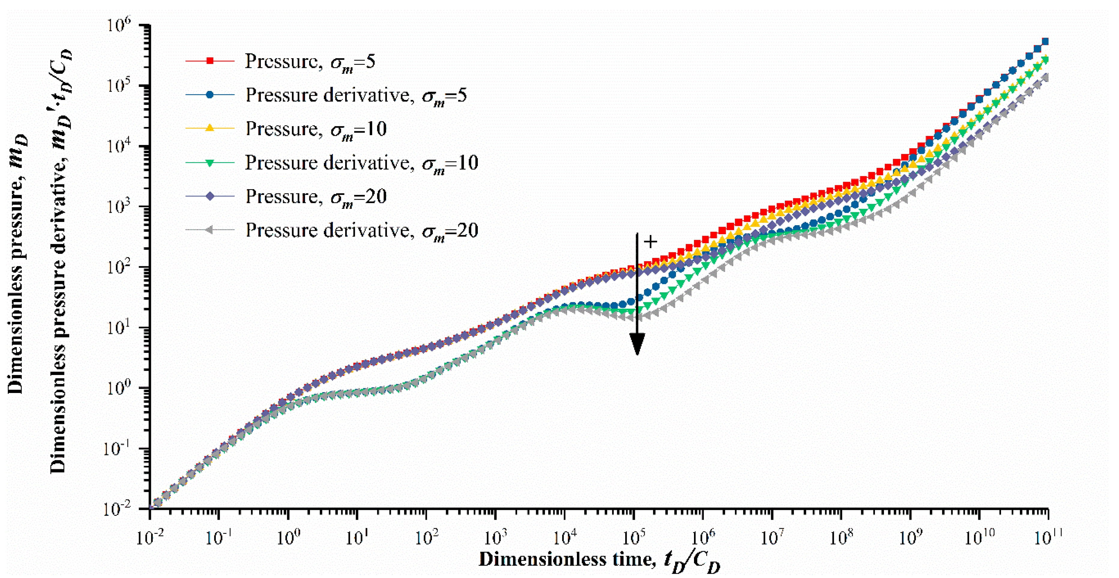
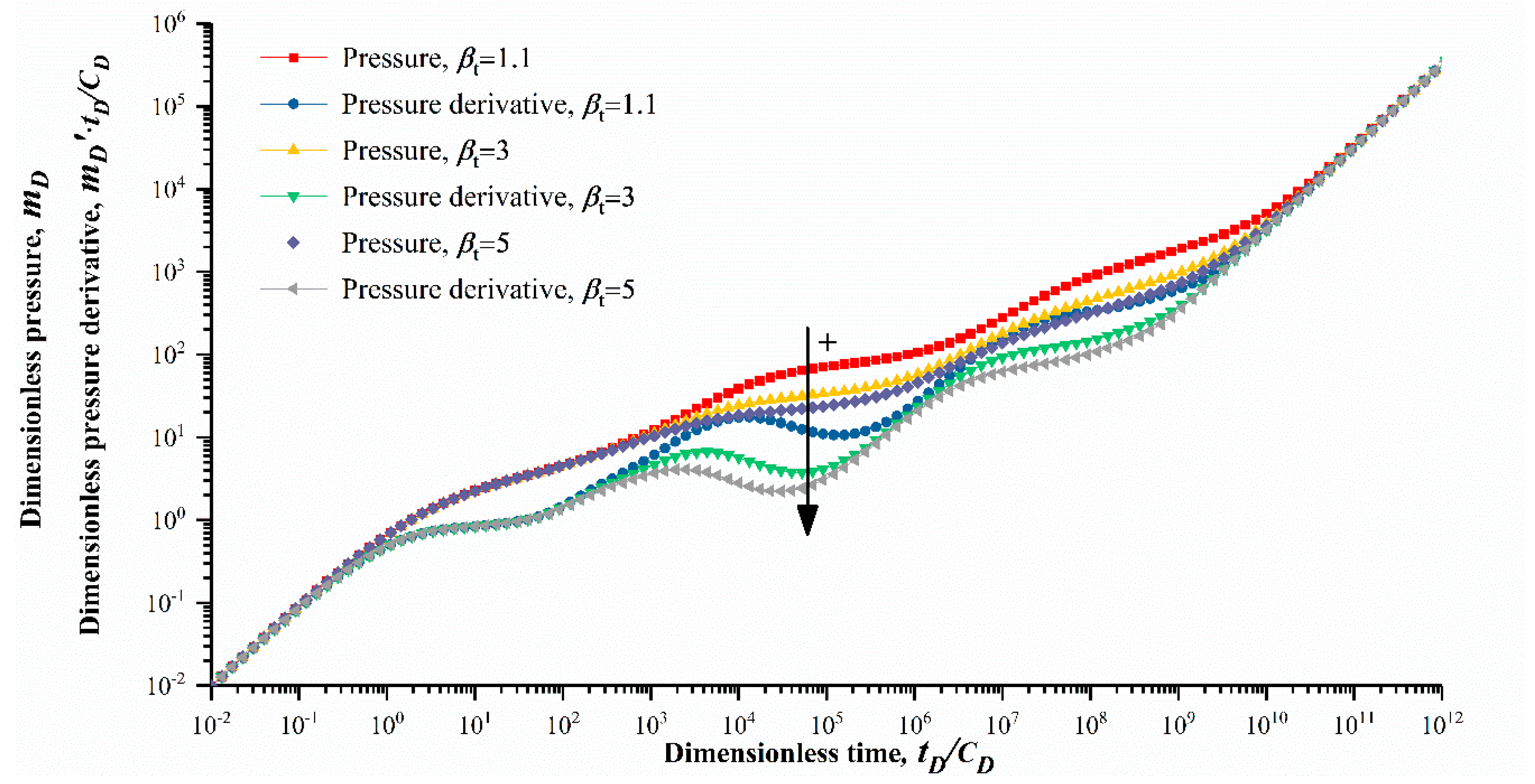
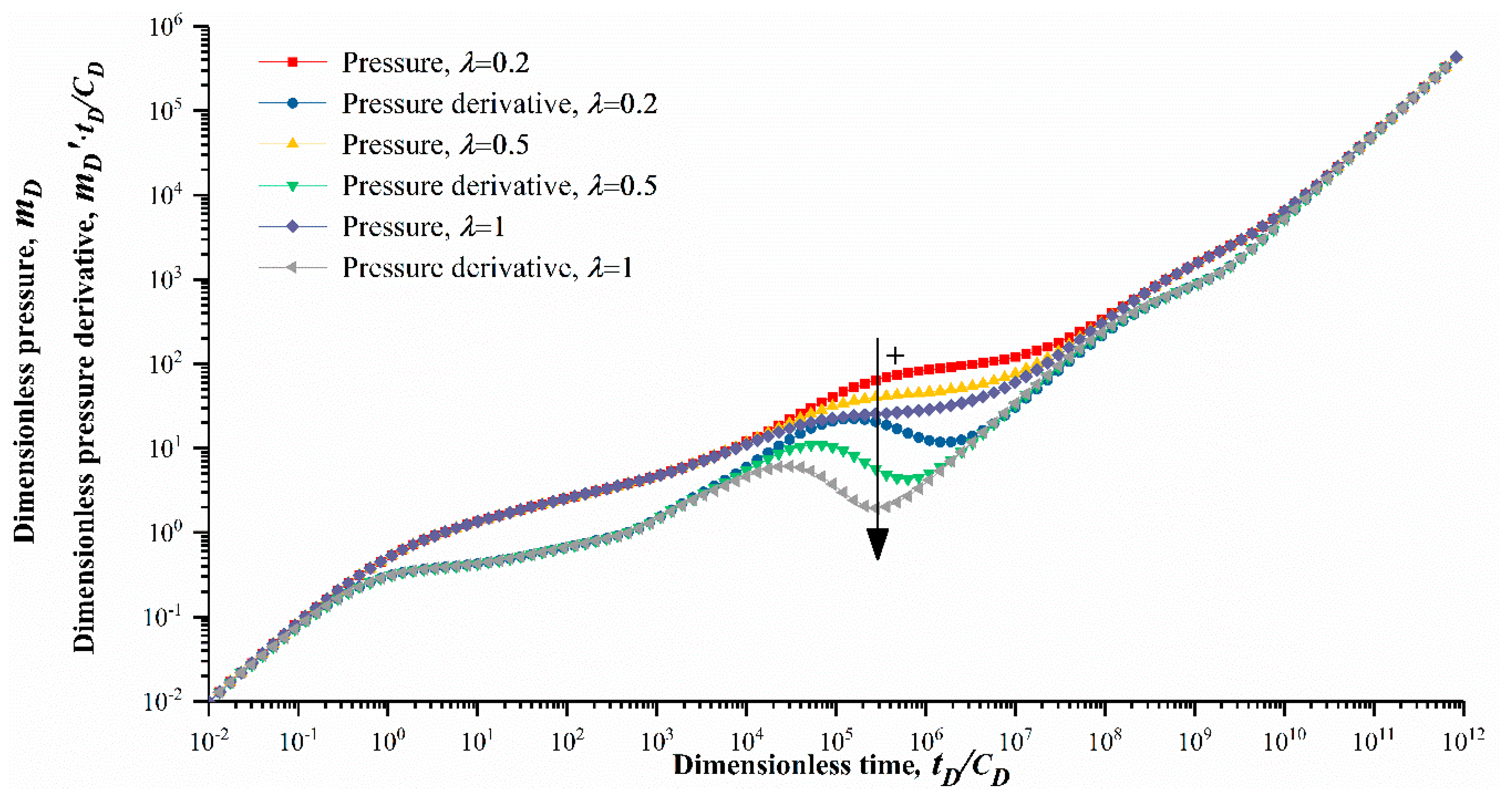
Figure 6, Figure 7 and Figure 8 demonstrate the influences of the adsorption factor, apparent permeability coefficient, and inter-porosity flow coefficient on the type curves of MFHWs. As shown in Figure 6, the adsorption factor mainly influences the position of the type curves at the inter-porosity flow stage. A larger adsorption factor represents a stronger adsorption and production capacity and therefore makes the “concave” appear wider and deeper on the type curves. Figure 7 shows the effect of the apparent permeability coefficient on the transient pressure response. The apparent permeability has a similar effect to that of the inter-porosity coefficient in Figure 8. The total seepage and diffusion ability of the shale matrix is represented by the apparent permeability coefficient. The smaller the apparent permeability coefficient or inter-porosity coefficient is, the later the “depression” appears on the type curves.

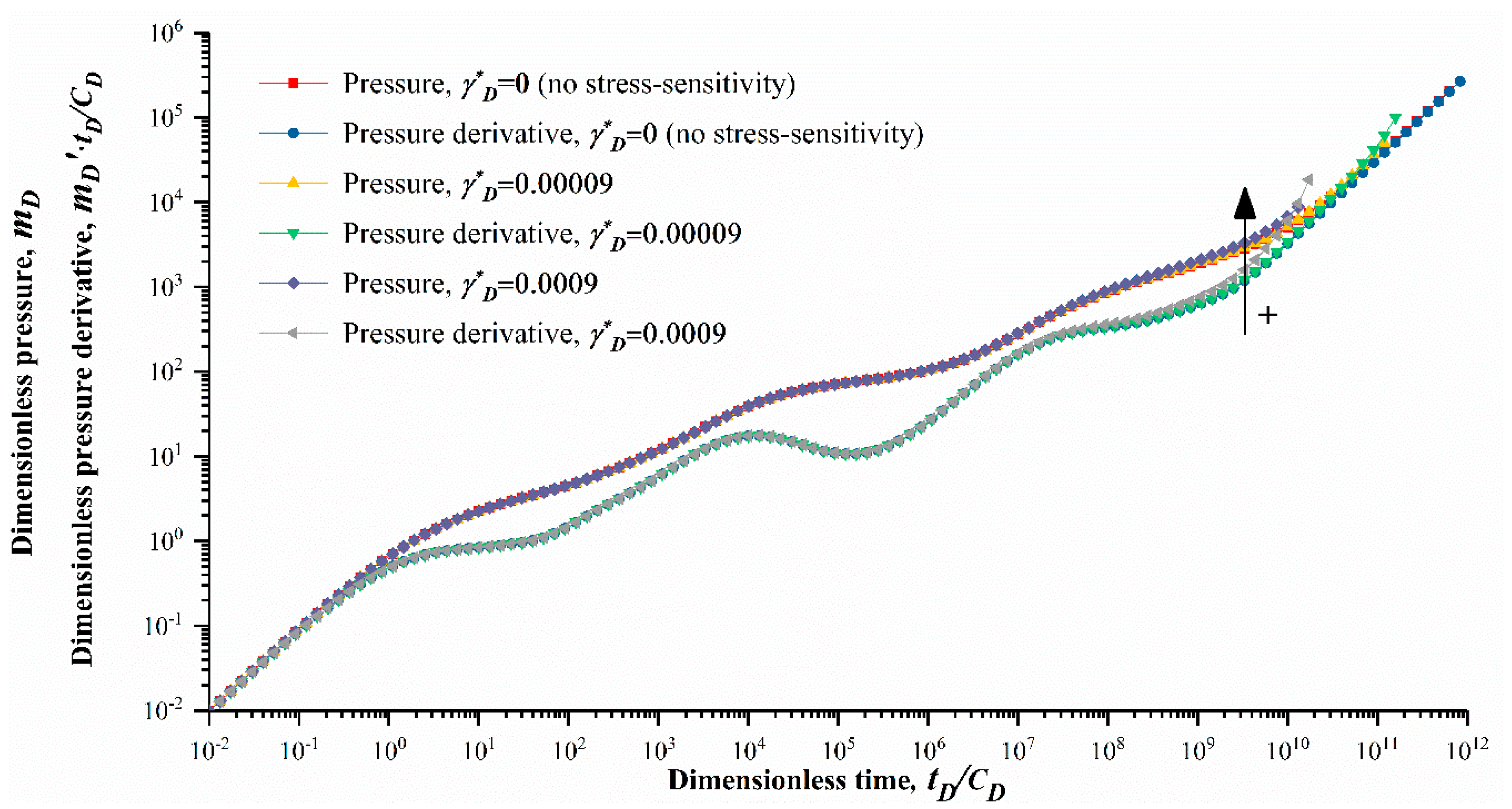
Figure 9 shows the impact of the stress sensitivity factor on the pressure-transient response of MFHWs. It can be seen that stress sensitivity affects the whole flow stage, and it has a greater impact in the late time period. The reason for this is that the pressure drop becomes greater in the late time period. The greater the stress sensitivity is, the higher the positions of the pressure and pressure derivative curves are. This depicts the weaker seepage capacity.

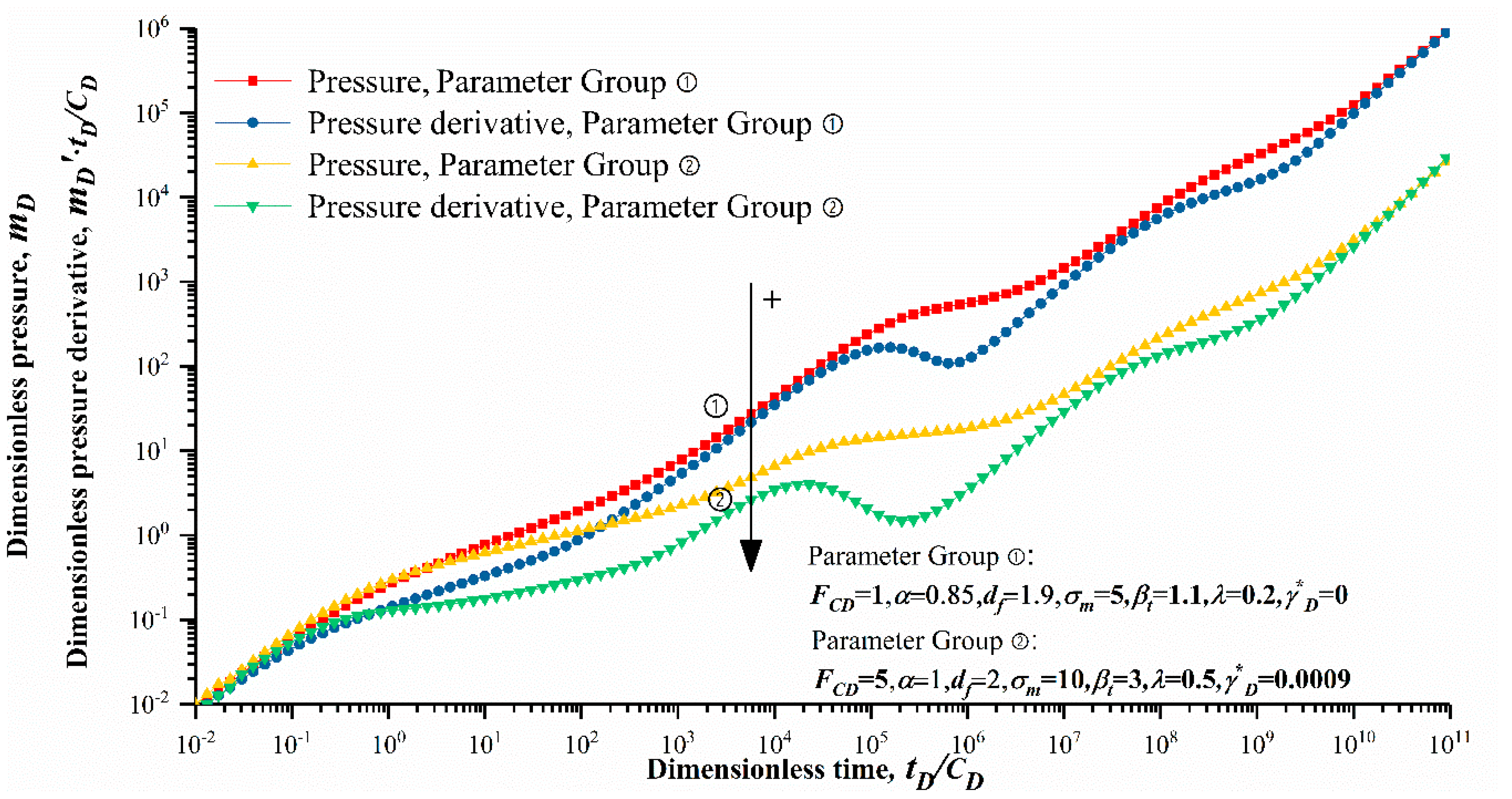
As shown in Figure 10, when all the factors are changed at the same time from a smaller parameter group ① to a larger parameter group ②, the positions of type curves for parameter group ② are obviously lower than the positions of type curves for parameter group ①. This indicates that when all the factors become larger, the final pressure drop becomes smaller. The reason for this is that most factors with greater values, such as $F_{\mathrm{CD}}$, $\alpha$, $d_f$ ${\sigma }_m$, ${\beta }_t$, and $\lambda ,$ can have positive effects by making the pressure consumption smaller, and only ${\gamma }_D^{*}$ has the opposite influence on pressure and pressure derivatives.

5. Case Study

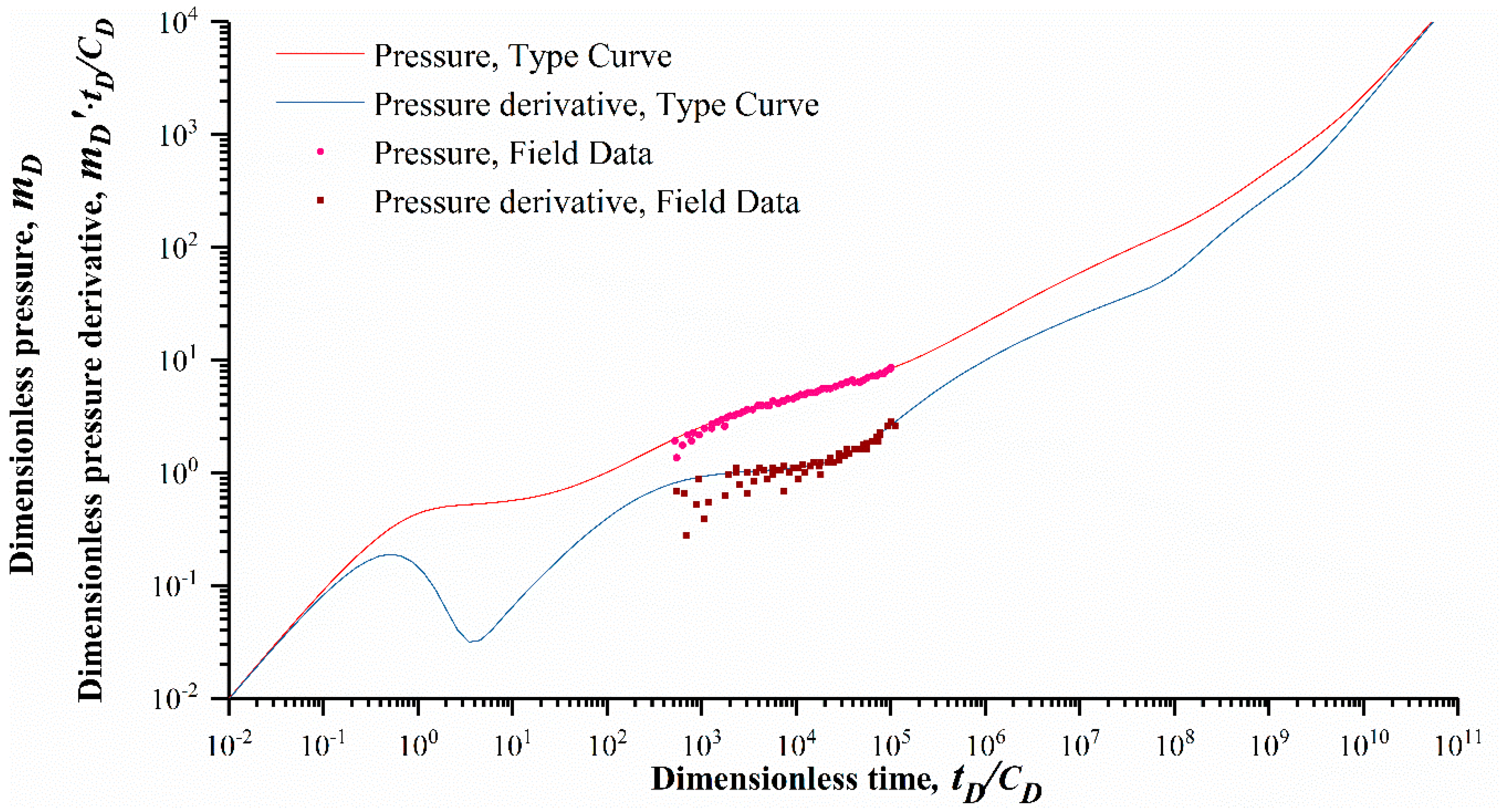
This section shows an application of the presented model in a fractured horizontal well (A1) of an actual shale gas field in the Sichuan basin, which has 12 fractures evenly distributed along its horizontal wellbore. The depth of well A1 is 880 m and the thickness of the shale layer is 76 m. The production was 2400 cubic meters per day for 16 h, and then it was shut down for 73 h during the pressure build-up test. For more details, refer to the related literature [16]. After transferring the build-up testing data to dimensionless forms, the actual log-log curves were plotted.

As shown in Figure 11, the improved five-region flow model proposed in this work was applied to match the build-up testing data and was able to perfectly match the real testing data by adjusting the relevant parameters. The results of the interpretation are listed in

Table 3. Interpretation results for the build-up test of well A1.

Parameter	Parameter Value
Half fracture length, xf	35 m
Inter-porosity flow coefficient, λ	λ = 0.1
Storage capacity coefficient, ω	ω = 0.05
Permeability of hydraulic fracture, kF	4000 mD
Fracture permeability in SRV, knf	0.0002 mD
Matrix permeability in regions, kim	k1m= k2m= k3m= k4m= 0.000005 mD
Absorption factor, ${\sigma }_m$	4
Diffusion factor(Apparent permeability coefficient), βt	1.5
Dimensionless stress-sensitive factor, ${\gamma }_{\mathrm{D}}^{*}$	0.00008
Anomalous diffusion exponent, α	0.7
Tortuosity index, θ	0.86
Hausdorff index, df	1.85

. The results reveal that hydraulic fracturing greatly increases the permeability of the fractured zone and produces complex induced fractures with fractal features.

6. Conclusions

In order to describe the flow retardation in complex fractures in a way that considers the SRV region with anomalous diffusion and fractal features, an improved five-region model was established in this work by introducing the time-fractional flux law. Based on the present model, type curves of pressure and pressure derivative without wellbore storage were plotted and five flow stages were identified: bilinear flow, first linear flow, inter-porosity and fractal-anomalous flow, second linear flow, and boundary control flow. The sensitivity analysis revealed that fractal-anomalous diffusion has a significant impact on pressure-transient behaviors. When the anomalous diffusion exponent decreased from 1 to 0.75, which indicates Darcy flow changing to anomalous diffusion, the pseudo-pressure had less depletion at the early linear flow stages, but this subsequently became greater. When the Hausdorff index changed from 2 to 1.8, greater pressure consumption was needed to achieve the same production. Additionally, stress sensitivity, absorption, and Knudsen diffusion showed non-negligible influences on the pressure-transient response. These effects cannot be ignored. Therefore, the typical five-region flow model which does not take the fractal-anomalous diffusion into account cannot be applied for heterogeneous multi-fractured systems. The present model can be used to provide a more accurate and appropriate interpretation of well-testing data to guide exploration and development.

References

- Taherdangkoo, R.; Tatomir, A.; Taylor, R.; Sauter, M. Numerical investigations of upward migration of fracking fluid along a fault zone during and after stimulation. Energy Procedia 2017, 125, 126–135. [Google Scholar] [CrossRef]
- Tatomir, A.; McDermott, C.; Bensabat, J.; Class, H.; Edlmann, K.; Taherdangkoo, R.; Sauter, M. Conceptual model development using a generic Features, Events, and Processes (FEP) database for assessing the potential impact of hydraulic fracturing on groundwater aquifers. Adv. Geosci. 2018, 45, 185–192. [Google Scholar] [CrossRef]
- Wang, J.; Jia, A.; Wei, Y.; Qi, Y. Approximate semi-analytical modeling of transient behavior of horizontal well intercepted by multiple pressure-dependent conductivity fractures in pressure-sensitive reservoir. J. Pet. Sci. Eng. 2017, 153, 157–177. [Google Scholar] [CrossRef]
- Tang, C.; Chen, X.; Du, Z.; Yue, P.; Wei, J. Numerical Simulation Study on Seepage Theory of a Multi-Section Fractured Horizontal Well in Shale Gas Reservoirs Based on Multi-Scale Flow Mechanisms. Energies 2018, 11, 2329. [Google Scholar] [CrossRef]
- Wang, H. Discrete fracture networks modeling of shale gas production and revisit rate transient analysis in heterogeneous fractured reservoirs. J. Pet. Sci. Eng. 2018, 169, 796–812. [Google Scholar] [CrossRef]
- Zhang, Q.; Su, Y.; Wang, W.; Sheng, G. A new semi-analytical model for simulating the effectively stimulated volume of fractured wells in tight reservoirs. J. Nat. Gas Sci. Eng. 2015, 27, 1834–1845. [Google Scholar] [CrossRef]
- Chen, P.; Jiang, S.; Chen, Y.; Zhang, K. Pressure response and production performance of volumetric fracturing horizontal well in shale gas reservoir based on boundary element method. Eng. Anal. Boundary Elem. 2018, 87, 66–77. [Google Scholar] [CrossRef]
- Wang, M.; Fan, Z.; Xing, G.; Zhao, W.; Song, H.; Su, P. Rate Decline Analysis for Modeling Volume Fractured Well Production in Naturally Fractured Reservoirs. Energies 2018, 11, 43. [Google Scholar] [CrossRef]
- Brown, M.; Ozkan, E.; Raghavan, R.; Kazemi, H. Practical solutions for pressure-transient responses of fractured horizontal wells in unconventional shale reservoirs. SPE Reserv. Eval. Eng. 2011, 14, 663–676. [Google Scholar] [CrossRef]
- Stalgorova, K.; Mattar, L. Analytical model for unconventional multifractured composite systems. SPE Reserv. Eval. Eng 2013, 16, 246–256. [Google Scholar] [CrossRef]
- Zhao, Y.-L.; Zhang, L.-H.; Luo, J.-X.; Zhang, B.-N. Performance of fractured horizontal well with stimulated reservoir volume in unconventional gas reservoir. J. Hydrol. 2014, 512, 447–456. [Google Scholar] [CrossRef]
- Deng, Q.; Nie, R.-S.; Jia, Y.-L.; Huang, X.-Y.; Li, J.-M.; Li, H.-K. A new analytical model for non-uniformly distributed multi-fractured system in shale gas reservoirs. J. Nat. Gas Sci. Eng. 2015, 27, 719–737. [Google Scholar] [CrossRef]
- Chen, D.; Pan, Z.; Ye, Z. Dependence of gas shale fracture permeability on effective stress and reservoir pressure: Model match and insights. Fuel 2015, 139, 383–392. [Google Scholar] [CrossRef]
- Guo, J.; Zhang, L.; Zhu, Q. A quadruple-porosity model for transient production analysis of multiple-fractured horizontal wells in shale gas reservoirs. Environ. Earth Sci. 2015, 73, 5917–5931. [Google Scholar] [CrossRef]
- Zhang, J.; Huang, S.; Cheng, L.; Xu, W.; Liu, H.; Yang, Y.; Xue, Y. Effect of flow mechanism with multi-nonlinearity on production of shale gas. J. Nat. Gas Sci. Eng. 2015, 24, 291–301. [Google Scholar] [CrossRef]
- Zhang, L.; Gao, J.; Hu, S.; Guo, J.; Liu, Q. Five-region flow model for MFHWs in dual porous shale gas reservoirs. J. Nat. Gas Sci. Eng. 2016, 33, 1316–1323. [Google Scholar] [CrossRef]
- Al-Rbeawi, S. Analysis of pressure behaviors and flow regimes of naturally and hydraulically fractured unconventional gas reservoirs using multi-linear flow regimes approach. J. Nat. Gas Sci. Eng. 2017, 45, 637–658. [Google Scholar] [CrossRef]
- Yuan, B.; Su, Y.; Moghanloo, R.G.; Rui, Z.; Wang, W.; Shang, Y. A new analytical multi-linear solution for gas flow toward fractured horizontal wells with different fracture intensity. J. Nat. Gas Sci. Eng. 2015, 23, 227–238. [Google Scholar] [CrossRef]
- Zeng, Y.; Wang, Q.; Ning, Z.; Sun, H. A Mathematical Pressure Transient Analysis Model for Multiple Fractured Horizontal Wells in Shale Gas Reservoirs. Geofluids 2018, 2018. [Google Scholar] [CrossRef]
- Zeng, J. Analytical Modeling of Multi-Fractured Horizontal Wells in Heterogeneous Unconventional Reservoirs. Master’s Thesis, University of Regina, Regina, Saskatchewan, 2017. [Google Scholar]
- Zeng, J.; Wang, X.; Guo, J.; Zeng, F. Composite linear flow model for multi-fractured horizontal wells in heterogeneous shale reservoir. J. Nat. Gas Sci. Eng. 2017, 38, 527–548. [Google Scholar] [CrossRef]
- Chen, C.; Raghavan, R. Transient flow in a linear reservoir for space–time fractional diffusion. J. Pet. Sci. Eng. 2015, 128, 194–202. [Google Scholar] [CrossRef]
- Ren, J.; Guo, P. Anomalous diffusion performance of multiple fractured horizontal wells in shale gas reservoirs. J. Nat. Gas Sci. Eng. 2015, 26, 642–651. [Google Scholar] [CrossRef]
- Albinali, A.; Ozkan, E. Analytical Modeling of Flow in Highly Disordered, Fractured Nano-Porous Reservoirs. In Proceedings of the SPE Western Regional Meeting, Anchorage, AK, USA, 23–26 May 2016. [Google Scholar]
- Wang, W.; Su, Y.; Sheng, G.; Cossio, M.; Shang, Y. A mathematical model considering complex fractures and fractal flow for pressure transient analysis of fractured horizontal wells in unconventional reservoirs. J. Nat. Gas Sci. Eng. 2015, 23, 139–147. [Google Scholar] [CrossRef]
- Fan, D.; Ettehadtavakkol, A. Semi-analytical modeling of shale gas flow through fractal induced fracture networks with microseismic data. Fuel 2017, 193, 444–459. [Google Scholar] [CrossRef]
- Raghavan, R.S.; Chen, C.-C.; Agarwal, B. An analysis of horizontal wells intercepted by multiple fractures. SPE J. 1997, 2, 235–245. [Google Scholar] [CrossRef]
- Al-Hussainy, R.; Ramey, H., Jr.; Crawford, P. The flow of real gases through porous media. J. Pet. Technol. 1966, 18, 624–636. [Google Scholar] [CrossRef]
- King, G.R.; Ertekin, T. Comparative evaluation of vertical and horizontal drainage wells for the degasification of coal seams. SPE Reserv. Eng. 1988, 3, 720–734. [Google Scholar] [CrossRef]
- Zhang, L.; Shan, B.; Zhao, Y.; Tang, H. Comprehensive Seepage Simulation of Fluid Flow in Multi-scaled Shale Gas Reservoirs. Transp. Porous Media 2017, 121, 263–288. [Google Scholar] [CrossRef]
- Cai, J.; Yu, B. Prediction of maximum pore size of porous media based on fractal geometry. Fractals 2010, 18, 417–423. [Google Scholar] [CrossRef]
- Cai, J.; Luo, L.; Ye, R.; Zeng, X.; Hu, X. Recent advances on fractal modeling of permeability for fibrous porous media. Fractals 2015, 23, 1540006. [Google Scholar] [CrossRef]
- Sheng, M.; Li, G.; Tian, S.; Huang, Z.; Chen, L. A fractal permeability model for shale matrix with multi-scale porous structure. Fractals 2016, 24, 1650002. [Google Scholar] [CrossRef]
- Cai, J.; Wei, W.; Hu, X.; Liu, R.; Wang, J. Fractal characterization of dynamic fracture network extension in porous media. Fractals 2017, 25, 1750023. [Google Scholar] [CrossRef]
- Chang, J.; Yortsos, Y.C. Pressure transient analysis of fractal reservoirs. SPE Form. Eval. 1990, 5, 31–38. [Google Scholar] [CrossRef]
- Acuna, J.; Ershaghi, I.; Yortsos, Y. Practical application of fractal pressure transient analysis of naturally fractured reservoirs. SPE Form. Eval. 1995, 10, 173–179. [Google Scholar] [CrossRef]
- Acuna, J.A.; Yortsos, Y.C. Application of fractal geometry to the study of networks of fractures and their pressure transient. Water Resour. Res. 1995, 31, 527–540. [Google Scholar] [CrossRef]
- Ozcan, O.; Sarak, H.; Ozkan, E.; Raghavan, R.S. A trilinear flow model for a fractured horizontal well in a fractal unconventional reservoir. In Proceedings of the SPE Annual Technical Conference and Exhibition, Amsterdam, The Netherlands, 27–29 October 2014. [Google Scholar]
- Caputo, M. Linear models of dissipation whose Q is almost frequency independent—II. Geophys. J. Int. 1967, 13, 529–539. [Google Scholar] [CrossRef]
- Molina, O.M.; Zeidouni, M. Analytical Model for Multifractured Systems in Liquid-Rich Shales with Pressure-Dependent Properties. Transp. Porous Media 2017, 119, 1–23. [Google Scholar] [CrossRef]
- Pedrosa, O.A., Jr. Pressure transient response in stress-sensitive formations. In Proceedings of the SPE California Regional Meeting, Oakland, CA, USA, 2–4 April 1986. [Google Scholar]
- Davies, B.; Martin, B. Numerical inversion of the Laplace transform: A survey and comparison of methods. J. Comput. Phys. 1979, 33, 1–32. [Google Scholar] [CrossRef]
Figure 1.
Schematic of physical models for hydraulically fractured horizontal wells. (a) The typical five-region flow model proposed by Stalgorova and Mattar [10]. (b) The improved five-region flow model (new model). Fracture half-length: ; width of the hydraulic fracture: ; distance from the hydraulic fracture to stimulated reservoir volume (SRV): ; no flow bound: .
Figure 2.
Transient pressure type curves of multiple fractured horizontal wells (MFHWs) in a shale gas reservoir.
Figure 3.
Effect of fracture conductivity on type curves.
Figure 4.
Effect of the anomalous diffusion exponent on type curves.
Figure 5.
Effect of mass fractal dimension on type curves.
Figure 6.
Effect of the adsorption factor on type curves.
Figure 7.
Effect of the apparent permeability coefficient on type curves.
Figure 8.
Effect of the inter-porosity flow coefficient on type curves.
Figure 9.
Effect of the stress sensitivity factor on type curves.
Figure 10.
Effect of characteristic factors on type curves (FCD, α, df, , βt, λ, and ).
Figure 11.
Type curve matching for well A1.