1. Introduction
Cites are responsible for more than 60% of the energy demand and about 70% of the CO
emissions worldwide [
1], more than half of the world’s population lives in cities [
2]. Therefore, buildings and their energy demand are one of the keys to an efficient reduction of emissions. To reach the ambitious goal of the European Union to reduce 80% of CO
emissions by 2050 compared to 1990 [
3], a range of measures and scenarios need to be analyzed and evaluated to identify suitable strategies.
In a first step, the current heat demand of the city under investigation is needed. There are different approaches and methods to simulate this demand, as described by Reinhart and Davila [
4], Frayssinet et al. [
5] or Li et al. [
6]. However, all the methods and studies reviewed there focus on the energy demand only, not on the energy generation. Allegrini et al. [
7] describe several tools and methods that can simulate district-scale energy systems, some of them also calculate the energy demand. Most of the studies and methods described focus on one or several related energy generation components which are modeled in great detail. Allegrini et al. state that tools are needed which run on simplified yet validated models to achieve faster results to support decision makers in early design stages on an urban level. 3D models of the buildings and cities under investigation can help to deliver more detailed information as the base for demand and supply simulations [
8,
9,
10].
The World Energy Outlook 2018 by the International Energy Agency [
11] states that electrical heating as well as heating systems supplied by gas continue to play a significant role in the future. In general, district heating systems are considered an important part of the transition to renewable energy generation, as they allow to use different (renewable) energy sources as inputs and facilitate storage [
12]. Two of the most promising renewable energy systems for urban areas at the moment are co-generation plants operated with renewable gas and HP operated with renewable electricity [
13,
14]. CHP are often used in district heating networks as they provide heat very efficiently and thus offer a significant contribution to the reduction of CO
-emissions [
15,
16]. Large HP in district heating networks have advantages over individual installations in buildings, as the heat can be stored in large storages as well as in the network itself. By this, surplus renewable energy can be used whenever it is available. With the development and implementation of 4th generation low-temperature district heating networks, the integration of HPs becomes a viable alternative. For the efficient use of this kind of heating network, the buildings need to be refurbished and use a heating system that can operate on low supply temperatures. In Sweden, about 10% of the heat needed in district heating networks is supplied by large HP [
17,
18]. Also, in Denmark, the goal is to be less dependent on fossil fuels by integrating HP in district heating networks [
19]. The city of Copenhagen wants to supply their district heating network in a CO
neutral way by 2025 [
20].
Another important step for reducing emissions is to use the solar irradiance to produce electricity with photovoltaic (PV) systems. There are several studies that show methods on how to analyze the PV potential in urban areas [
21,
22]. Most of the studies investigating the PV potential are based on the 3D geometry of the buildings and their roofs [
23,
24,
25,
26] since knowing the exact roof shape and orientation helps to calculate more accurate values for the PV potential energy yield.
In this study, calculation models for district heating systems with either CHP units or large HP are developed. Subsequently, heat demand, PV potential, and both energy generation systems are assessed and compared for a small town in Southern Germany. For this modeling task, the urban modeling tool SimStadt [
27] is used to analyze several hundred buildings in parallel.
2. Methodology
For the development of different energy system scenarios, the heat demand of the case study town needs to be calculated first. Additionally, the local PV potential needs to be determined to assess the possible local electricity production. Then, energy generation models need to be developed to dimension and compare systems to meet the heat demand calculated beforehand. In this section, first the simulation environment SimStadt is explained and how it calculates heat demand and PV potential. Then, the development of two models for energy generation systems is shown in detail.
2.1. Simulation Environment
The analyses in this paper are made with the simulation platform SimStadt, using an internal connection to the simulation engine INSEL 8.2 [
28]. Both SimStadt and INSEL are under development at the University of Applied Sciences Stuttgart.
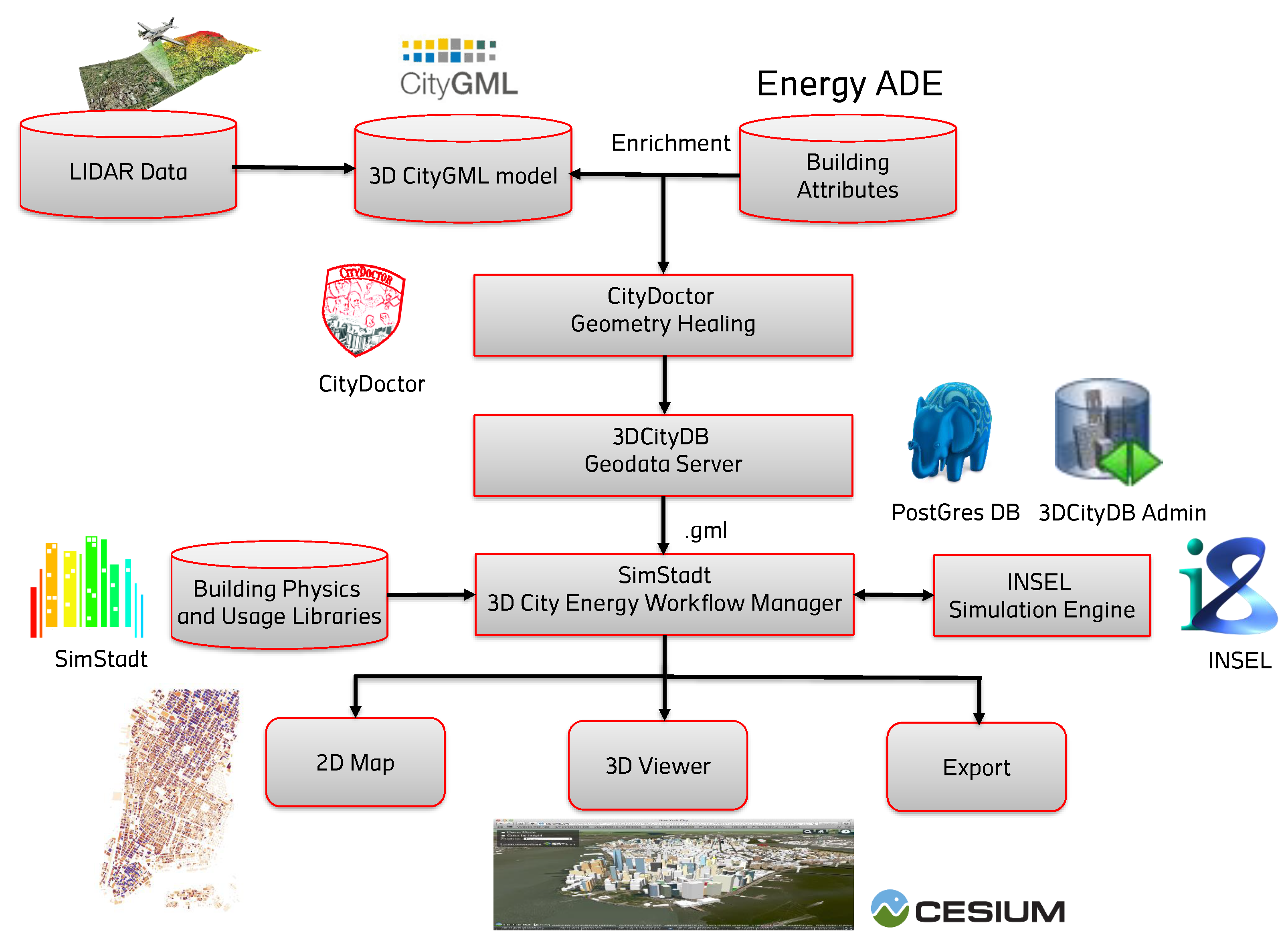
Figure 1 shows the simulation environment graphically.
The upper part of
Figure 1 describes the generation of 3D CityGML models from LIDAR data [
29] and the possible enrichment of the models with building attributes e.g., from municipal sources or the EnergyADE [
30]. The CityGML format can depict existing environments such as buildings, roads, and landscape. Building models can be available in five different level of details (LOD); LOD0 as only a planar shape, LOD1 where the building is represented as a cube with an average building height and a flat roof, LOD2 which has more detailed information about building heights and roof shapes, LOD3 introduces windows and LOD4 has a detailed interior design and information about wall thicknesses (see
Figure 2).
The CityGML model is then quality checked by the tool CityDoctor, which is under development at the University of Applied Sciences. This tool checks the 3D CityGML model and can repair possible geometrical errors, e.g., open polygons which prevent the buildings from being recognized properly are closed. The model can then be stored in the 3D CityDB geodata server or directly used for simulation in SimStadt.
SimStadt has a graphical user interface (GUI) and consists of different work flow steps that use information given in the CityGML model, building physics, and usage library and from weather databases. The geometry of every individual building from the CityGML file is used and linked to the different libraries in the SimStadt platform.
The building physics library is based on the typology developed by the German Institute IWU (Institut Wohnen und Umwelt) [
32], which classifies buildings according to their type and year of construction. For each building type and period, there is a typical building with its respective wall, roof, and window properties. These properties are applied to the actual building geometry and SimStadt then calculates individual u-values for each building. Additional to the properties of existing buildings, different refurbishment scenarios are available in the building physics library.
The usage library is based on several German norms and standards, focusing on heating set point temperatures, occupancy schedules and internal gains that are different according to the usage (residential, office, retail, etc.) of each building.
INSEL is the simulation engine behind SimStadt and can be purchased from doppelintegral [
28]. INSEL is a block diagram simulation system for programming applications for renewable energy technologies. It has some ready-made simulation models included, but it is also possible to design own model extensions or entirely new models.
The results from the SimStadt simulations can be visualized in 2D maps, on a 3D globe [
33] or the building-specific results can be exported in a .csv-file.
SimStadt is still in a beta status and therefore not publicly available; however there are several studies and publications where the calculation method of SimStadt is described and the tool was used to calculate the heat demand or PV potential of different case studies [
27,
34,
35,
36,
37,
38,
39,
40].
2.2. Heat Demand Analysis
SimStadt calculates the heat demand of a town or city quarter as a monthly energy balance according to the German standard DIN 18599 [
41]. It uses the information in the building physics and usage libraries to determine the heat transmissions through the building envelope for each building according to their building type and age.
For the dimensioning and calculation of the generation systems that are the focus of this paper, however, more time-resolved values are needed. Therefore, the monthly values are transferred into hourly values, depending on the hourly outside temperature and the desired room temperature of 20 °C. This process is described in the German standard VDI 4710 [
42]. The heating period in Germany commonly is from October to April; in summer months, the heating system is shut down entirely, so the heat demand (excluding domestic hot water demand) is zero. Additionally, there is a nightly shutdown from 0 to 6 am, where the minimum temperature is 15 °C. Nightly shutdown is a common practice to reduce the heat load and is included in several German norms, e.g., in the DIN V 18599 which also describes the monthly energy balance calculation.
2.3. Photovoltaic Electricity Generation
The PV potential can also be simulated with SimStadt and the same CityGML file from the heat demand analysis is used as input data in combination with the irradiance data of the location. In the first simulation steps, SimStadt is using the 3D CityGML Model to determine the inclination and azimuth for every roof area and calculates the solar irradiance on those surfaces. Different radiation models can be applied, in this case the Hay algorithm is used [
43]. It does not take shading of trees or other buildings into account. However, since the building density is quite low and the individual buildings are of similar height, this is an acceptable limitation and trade-off between accuracy and computation time.
The next step is the parametrization for the PV potential analysis. It consists of the building surface suitability and PV system parameters. Suitability settings include for example, the minimum surface area and the minimum annual irradiation on the roof, at which a roof is determined as suitable for a PV system installation (default: ≥20 m
/950 kWh/m
a). The PV system parameters include among others the ratio of the module area to the roof area (default: 30% for flat roofs to reduce shading, 40% for tilted roofs to account for roof windows, chimneys etc.); The module tilt was chosen as 20° for a south-facing installation on a flat roof in Germany, as this represents a good compromise of maximum irradiance, optimal row spacing (shading), self-cleaning and back-ventilation of the PV modules [
44]. The default module efficiency and performance ratio are 17% and 80%, respectively. Based on those parameters the yearly energy yield for every suitable roof area is calculated.
With the current SimStadt version, only the annual and monthly cumulated PV energy yield can be simulated. Therefore, with the help of the simulation engine INSEL 8.2, an hourly PV load profile was generated in this study using the same weather data and PV system parameters as in SimStadt. Then, the roof areas of the area under investigation are divided into four roof types (tilted roof orientations (east/south/west) and flat roofs). The average inclination and azimuth of every roof type is calculated, as well as the share of the surface area of every roof type. The PV load profile in INSEL considers the same roof type shares with their average inclination and azimuth. The annual PV yield from SimStadt can then be split per hour via the load profile from INSEL.
3. Extension of the Simulation Environment and Addition of New Functionalities
The simulation environment described above has been developed over several years and different projects at the University of Applied Sciences Stuttgart and was adapted in some ways for the analyses in this study. The focus of this paper is the methodology for the addition of energy generation systems to the simulation environment. Add the end of this section, the current simulation sequence is explained in detail. First, the added functionalities themselves are described.
3.1. Heat Pump Generation
The whole HP system is developed in the INSEL simulation environment. A simplified representation of the model is shown in
Figure 3.
Depending on the type of HP used, the air, water, or ground temperature of the heat source is needed as an input in an hourly resolution. Also needed is specific HP data such as coefficient of performance (COP) and power characteristics dependent on the heat source temperature and supply temperature of the heating network, which are usually provided by the manufacturer. The HP is modeled by a polynomial fit to this manufacturer data as a function of source and sink temperature. Finally, the monthly heat demand that is calculated in SimStadt and then transferred to hourly values is needed as an input. The months of the heating season can be adjusted in the model to control the operation time of the HP. Also, the needed supply temperature of the heating network can be varied depending on the system configuration.
Different key performance indicators (KPI) are analyzed as outputs of the model. The most important results are the information about the HP performance such as hourly or annual COP and heat generation. Data on the storage usage, hourly fill level, overflow or deficit of storage are also given as outputs. Additionally, values for heat losses (both for the distribution and storage losses) as well as the actual heat demand including those losses are provided for every time step.
3.2. District Heating Network and Central Storage
Additional to the HP, a large central storage is included in the system model to reduce the operating hours of the HP. The storage is sized to supply the average total heat load for three hours. This amount of time is chosen because of the utility blocking time, where the utility company is allowed to stop providing electricity to the HP for two hours in a row for a maximum of three times a day. The additional hour provides extra reserves in case of multiple blocks in a short period of time.
The heat demand is directly met from the storage. If the storage level is lower than 20% of its full capacity, the HP switches on to both meet the current demand and fill up the storage. As soon as the storage level reaches 80% of its full capacity, the HP switches off. With this control, it is ensured that the generation system does not switch on and off all the time, especially in spring and fall months when the demand can be met by the storage alone for a few hours in a row. Storage losses are included and calculated for a steel tank with 10 cm insulation.
Distribution heat losses are dependent on the length of the piping and the supply temperature and are therefore calculated in the model according to these two parameters. The losses are calculated with a simple steady-state model, using double piping with 5 cm insulation. The resulting losses are validated with other sources [
45,
46].
3.3. Co-Generation
The co-generation system is modeled very similarly to the HP simulation model shown in
Figure 3. Most of the parameters remain unchanged (e.g., the storage size and losses, distribution losses, and supply temperature, heating season, and the hourly heat demand). In this model the co-generation unit is operated in a heat-controlled mode and the electricity is seen as the by-product. As input for the CHP unit, the technical information from the manufacturer such as efficiency and nominal power are needed.
For the dimensioning of the co-generation unit, the annual load duration curve of the bulidings under investigation is analyzed. The choice of CHP operating hours is based on current economic feed-in conditions in Germany, where co-generation units should have at least 4000 full load hours to be able to operate cost efficiently. This corresponds to a rated output of the CHP unit to cover 20 to 25% of the maximum heat load [
47]. With this typical marked-based design, a coverage of about 50–75% of the annual heat demand of a district heating network is usually achieved [
48]. The rest of the demand that cannot be met by the CHP is provided by gas boilers. This mode of operation is very efficient to meet the peak demand [
49], since gas boilers can easily and often switch on and off without negative effects on their efficiency.
3.4. Current and Future Calculation Sequence
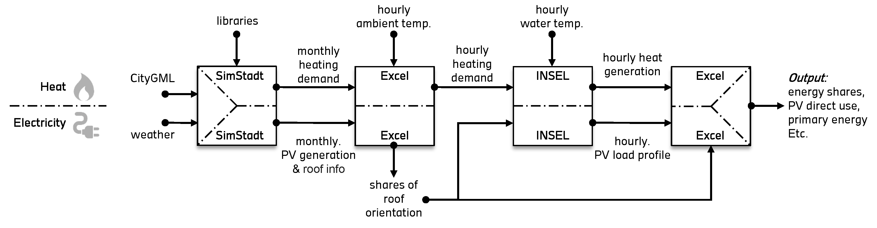
So far, the new functionalities are not yet added to the SimStadt platform itself and therefore, different tools need to be used to calculate each step. The calculation sequence needed in this study is shown in
Figure 4.
In the first part, different libraries, a weather data set specific to the location and the CityGML file of the area under investigation are needed as inputs in SimStadt. There, the monthly heat demand and PV generation as well as the information about the roof orientation, is given as outputs. This sequence is described in
Section 2.2 and
Section 2.3.
At present Microsoft Excel (or any other spreadsheet tool) is still needed as an interface between the SimStadt simulation results and the INSEL models simulating the hourly energy supply systems to transfer monthly values to hourly values, as described in
Section 2.2.
The hourly PV energy yield must be determined from the monthly values and the hourly profile, which is calculated in INSEL with the shares of the roof orientation, as described in
Section 2.3.
The results of the INSEL energy generation calculation then need to be exported to Microsoft Excel again for aggregating, analyzing, and visualizing the data output at the end. In the future, this whole process will be integrated as one work flow sequence into SimStadt.
4. Application to Case Study
The proposed methodology is applied to a small town in Southern Germany in the administrative district of Ludwigsburg, which belongs to the metropolitan area of Stuttgart. Since 2015, the district council of Ludwigsburg decided on a climate protection concept to determine the possibilities for reducing CO
emissions, to acquire subsidies and financial support based on a catalogue of measures, and decided on the overall goal to make the district climate-neutral by 2050 [
50].
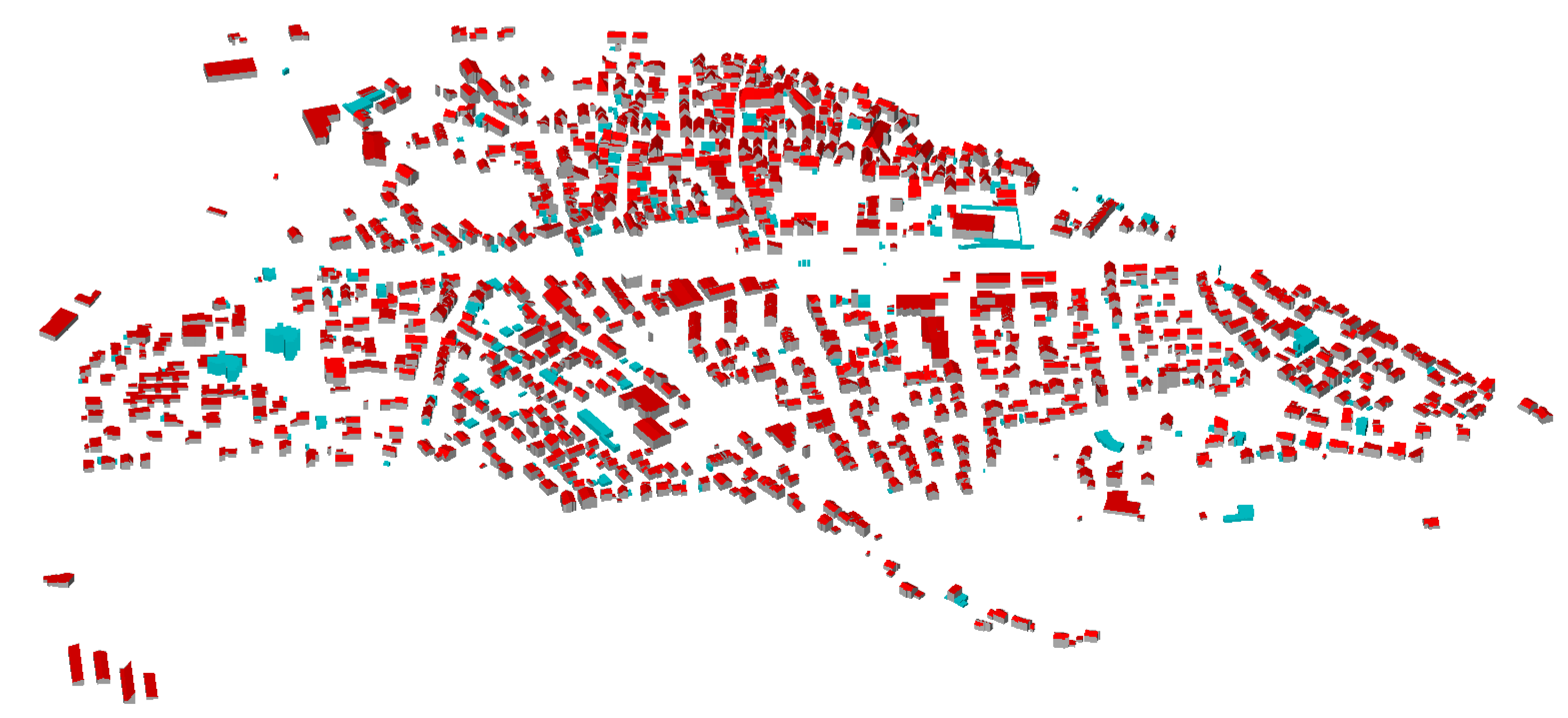
The town Walheim in the district of Ludwigsburg that is used as a case study in this analysis has around 3200 inhabitants. Next to Walheim flows the river Neckar, which is the second biggest river in the state of Baden-Württemberg. 1610 buildings are contained in the 3D CityGML model that is used for the simulations (see
Figure 5). This leads to a moderate size of the CityGML file and consequently short computation times.
All these factors are very good prerequisites that make Walheim an ideal case study for the application of this methodology.
Most of the buildings are in LOD2, but some of the buildings are represented only in LOD1 (blue in
Figure 2), so their actual roof shape is not known. 46% of the buildings are garages or sheds that are not heated. The remaining 872 buildings with a total footprint area of 109,919 m
are mainly residential buildings (89%), the rest are either used for industry, offices or retail.
For this study, all buildings are assumed to be refurbished according to the current German Energy Saving Ordinance EnEV 2016 [
51]. This assumption is needed to be able to simulate low-temperature district heating for all buildings in the town. Of course, this kind of large-scale refurbishment cannot be expected to take place in just a few years but it fits together nicely with the goals of the district of Ludwigsburg of becoming climate-neutral by 2050. Additionally, there are special programs and incentives from the KfW (Kreditanstalt für Wiederaufbau-German Reconstruction Loan Corporation) to promote building and city quarter refurbishments.
In a first step, the monthly heat demand of every building in the town of Walheim is calculated with SimStadt.
Table 1 shows the cumulated heat demand for all buildings of Walheim for every month.
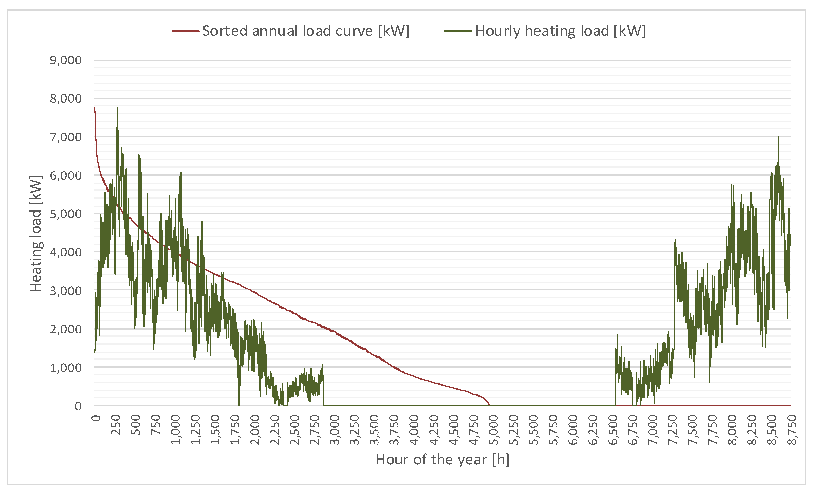
Then, the monthly values are transferred into hourly values as described in
Section 2.2. The hourly demand of each building is cumulated for each time step and ordered in a sorted annual heat load curve according to the value of the heat demand of each time step (see
Figure 6). The total annual heat demand of Walheim amounts to approximately 12,500 MWh/a with a peak load of 7767 kW in January. The considered heating season is October until April. Domestic hot water is not included in this assessment.
In this scenario, as many photovoltaic (PV) modules as possible are put on all suitable roofs of all buildings in Walheim. The German Erneuerbare-Energien Gesetz (EEG, renewable energies law) [
52] says that PV systems smaller than 10 kW do not have to pay additional fees when they feed PV electricity to the grid. Therefore, most PV systems on residential buildings are smaller than that, even though there might be space left on the roofs to place additional PV modules. Renowned German scientist Volker Quaschning addresses this issue [
53] and demands that all usable roof spaces should be used for PV electricity generation.
The PV potential simulation is carried out as it is described in
Section 2.3. The buildings in the CityGML file that are only available in LOD1 are excluded from the PV potential analysis, since their roof shape is not known. Therefore, the orientation cannot be determined.
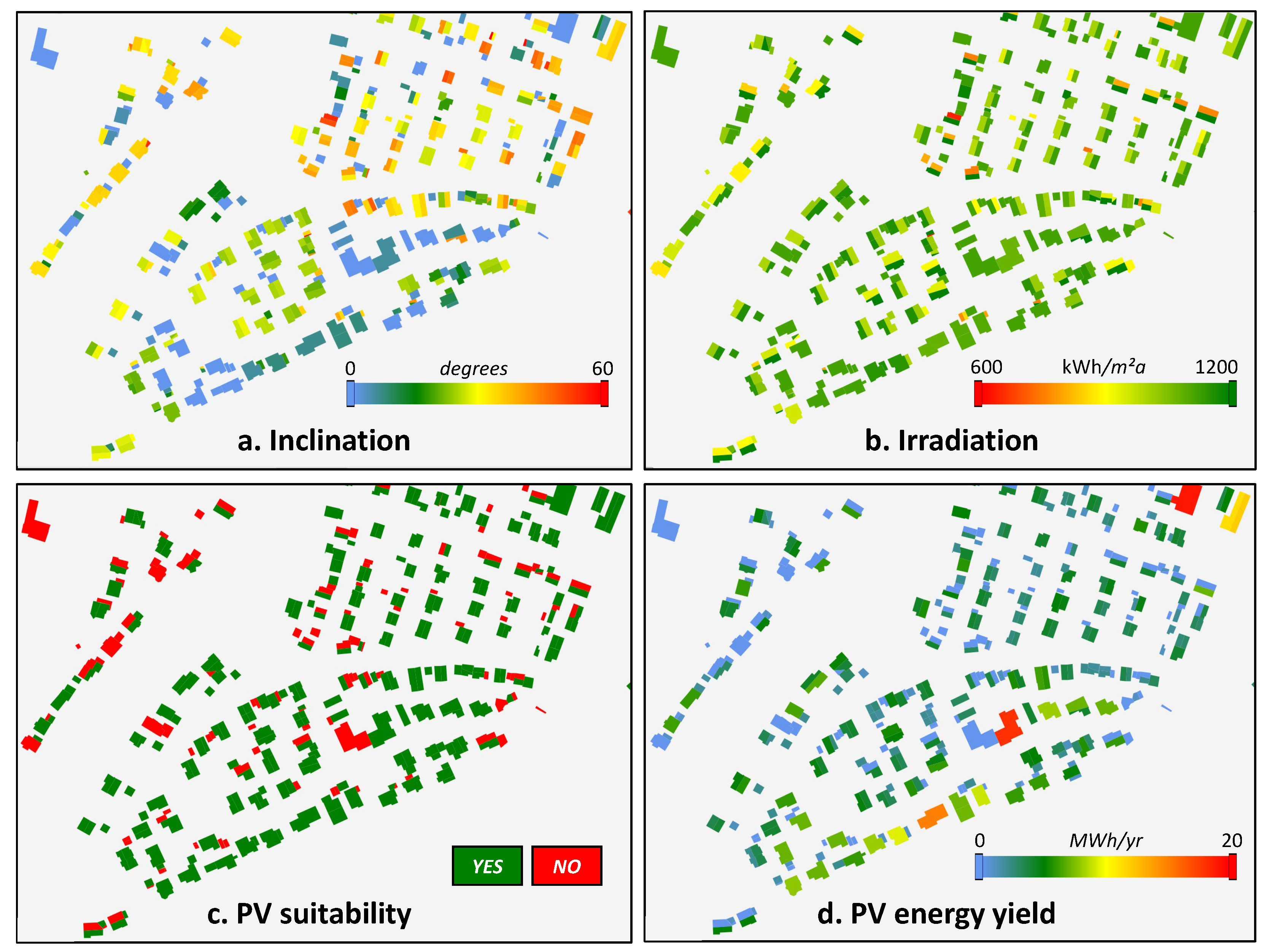
According to the SimStadt PV simulation this results in 1470 suitable roof areas for Walheim, with a total nominal power of 6417 kWp and an annual energy yield of 6043 MWh.
Figure 7 shows the simulation results of a part of Walheim for
(a) inclination of the roofs in [°]
(b) annual sum of global irradiation in [kWh/ma]
(c) the PV suitability of the roof according to the applied parameters and restrictions and
(d) the total annual PV energy yield of each roof in [MWh/a].
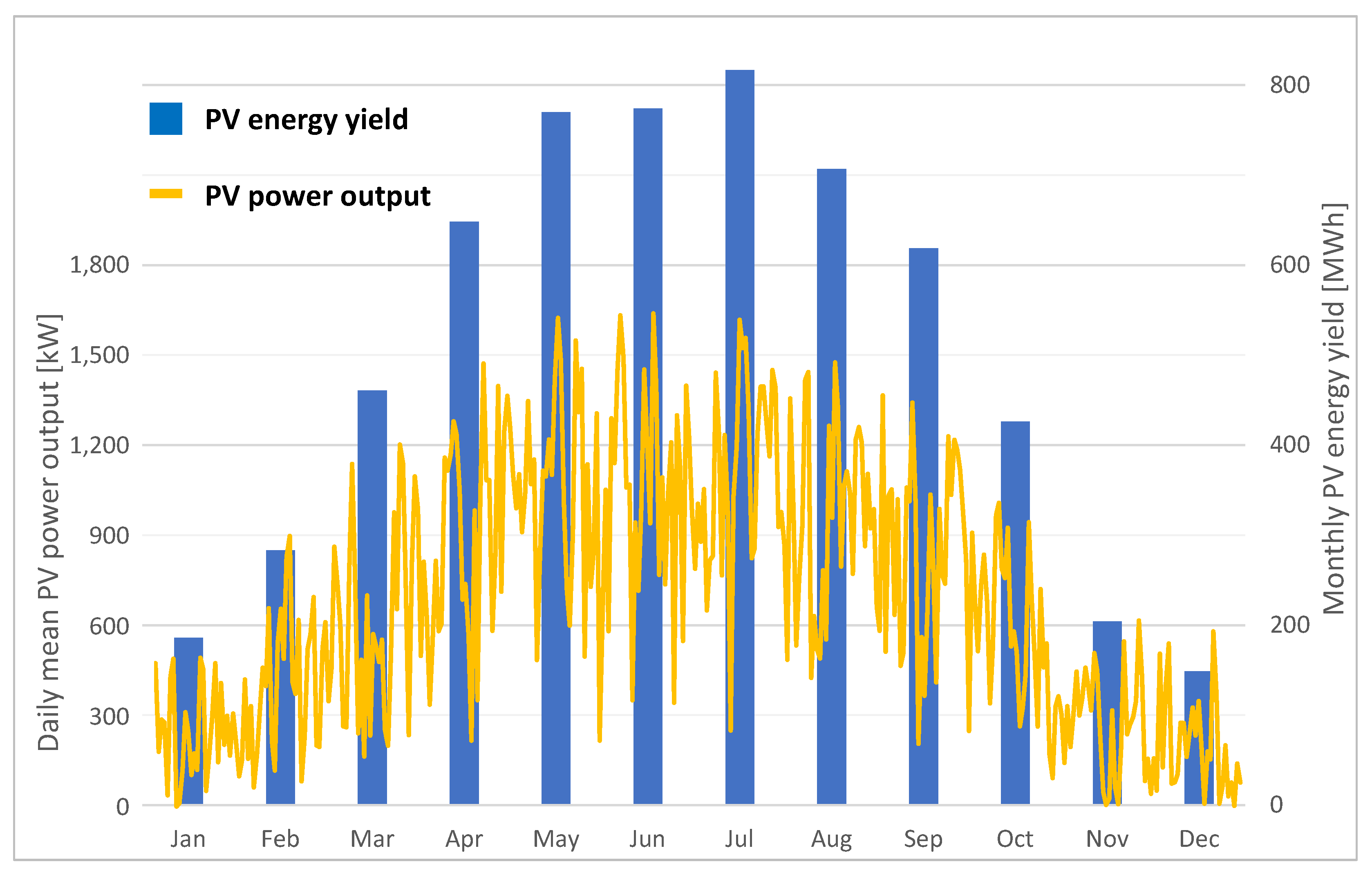
Figure 8 shows the PV power output and monthly energy yield over the course of one year. The monthly PV energy yield of all suitable roofs in Walheim combined is calculated in SimStadt (blue) and the daily mean PV power output in Walheim is shown in yellow, which is calculated with the specific PV load profile in INSEL.
The sorted annual heat load from
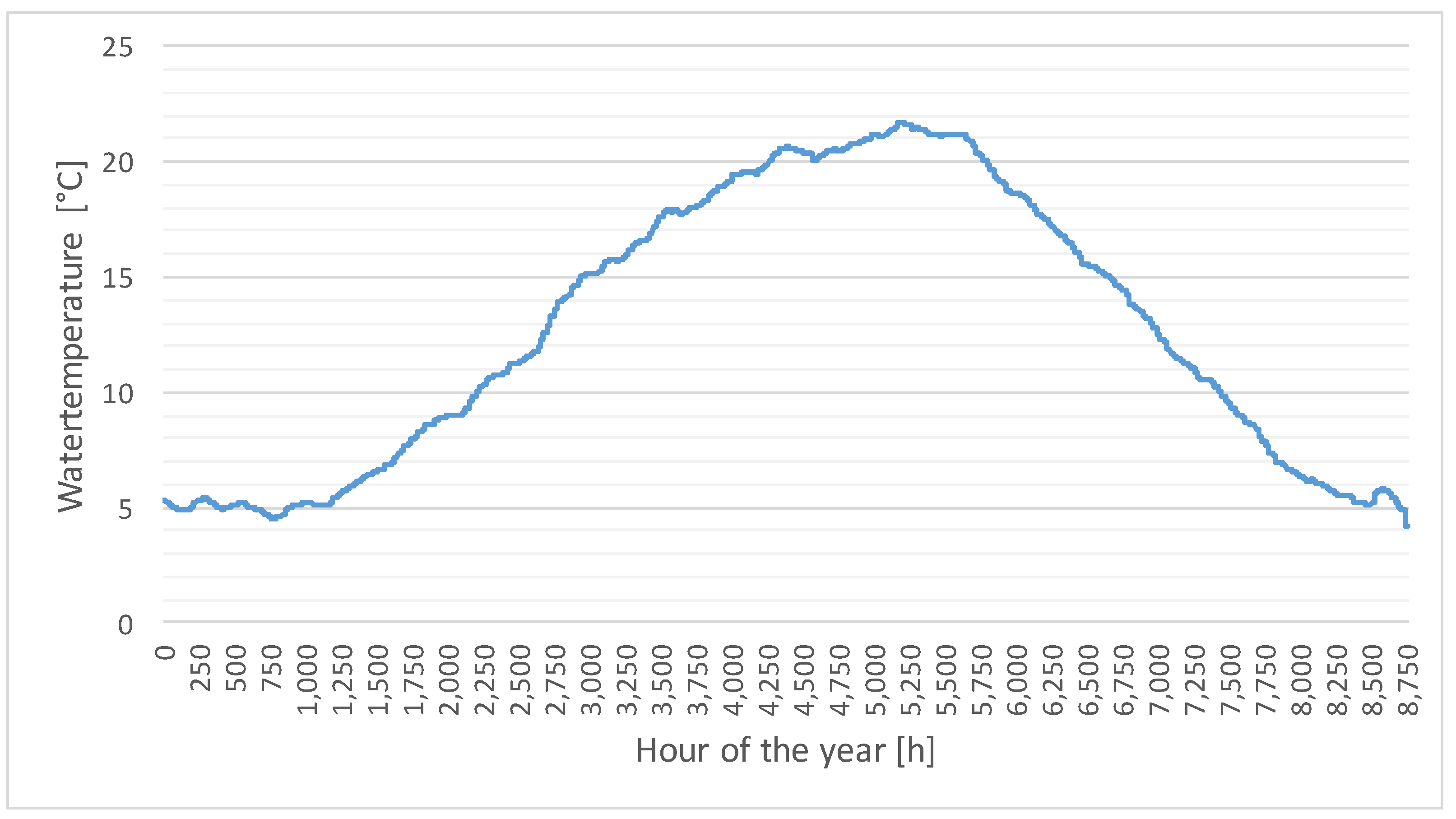
Figure 6 is used to choose the appropriate HP to match the demand of Walheim. Since the river Neckar flows directly next to the town, it serves as the heat source for the HP. The average daily water temperature between 1988 and 2014 at the measuring point in Besigheim, which is only a few hundred meters from the town of Walheim, varies between 4.21 °C in December and 21.71 °C in August (see
Figure 9).
Since the HP are the only source of heating energy for the network and are therefore in a monovalent operation mode, several large industry heat pumps need to be used in this case to supply the whole town of Walheim. After extensive market research, the IWWS 960 ER1a from Ochsner Energie Technik was selected. It is a water-water industry HP and has a nominal heat output of 966 kW. This size is ideal, since eight of the aforementioned HP can meet the peak load of 7767 kW.
Distribution heat losses are dependent on the length of the piping and are therefore calculated according to the total length of the network, which is assumed to be 12 km. Since the supply level of the heating network is only 45 °C, the mean heat losses of 106 kWh/h for the whole network are rather low with 7.5% on average. The temperature of the heating network can be chosen to be this low, because all the buildings connected to the network have been refurbished to a low-energy standard as well as low-temperature heating systems before.
The storage is set to supply the average annual load of the town of 1431 kW for three hours which leads to a size of 15 m in height and a diameter of 4 m of the insulated steel tank. Assuming a discharge temperature difference of 20 K (supply temperature to the network 45~°C, return temperature 25 °C), this results in 4314 kWh storage capacity. Storage losses of 0.851 kWh/h are included in the model.
Based on the dimensioning guidelines described in
Section 3.3, a co-generation unit within the range of 2000 kW nominal heat output is selected to supply the heat demand of the town of Walheim. The electricity generated by the CHP is assumed to be fed into the grid.
Since in this study both biogas (from fermentation of biomass or waste water sludge digestion) and gas from power to gas systems (P2G), where surplus electricity is used to produce gas from water with electrolysis are considered as fuel for the CHP, a unit of the manufacturer 2G was selected, which can be operated with both fuels with only a few technical changes (CHP Type: 2G avus 2000c). For natural gas and gas from P2G the nominal heat output of this CHP is 1977 kW with a thermal efficiency of 43.2% and the nominal electrical power output 2000 kW with an efficiency of 43.7%. In the case of biogas, the overall efficiency of the unit is 2.1% lower, which corresponds to 2009 kW/42.5% on the thermal side and 2000 kW/42.3% on the electrical side. The rest of the heat demand that cannot be met by the co-generation unit needs to be supplied by central gas boilers. To ensure the highest possible security of supply, two gas boilers with a nominal power of 4000 kW with an efficiency of 95% each are used. Thus, in the case of maintenance work on the CHP, the gas boilers can cover the entire heat load.
5. Results of Two Scenarios for Energy Generation Simulation
The overall results for the energy generation of both system simulations are compared in
Figure 10. The eight HP with a maximum heating power output of 8354 kW can generate 94% of the needed heating energy in only 1890 h. The HP system can store a large amount of heat and use this heat at other times to meet the demand. The heat that can be stored corresponds to the area between the gray and yellow lines in
Figure 10.
The CHP unit with a heating power output of constantly 2000 kW runs for 4012 h but only supplies 61% of the heat, the rest needs to be produced by the gas boilers. These shares correspond to 8024 MWh from the CHP unit and 5058 MWh or 39% from the gas boilers. The CHP system cannot store as much heat as the HP system because most of the produced heat is used directly. This is due to the lower nominal heat output of the CHP that produces less surplus heat compared to the eight HPs, even though the same storage size is used. This can be seen in
Figure 10 as the area between the blue and yellow lines.
Table 2 shows the KPI for the two systems. The heat demand is the same for both system designs, the heat losses slightly differ because the CHP system can store less heat in the storage and has therefore lower storage losses.
Electricity yield from PV is the same in both scenarios, in the CHP scenario, additional electricity is produced when the CHP is running. All electricity that is not directly used by either the HP or the P2G process is assumed to be fed to the grid. The remaining electricity needed for operation of either system is assumed to come from the grid.
The CHP unit can either be operated with biogas or with gas from power to gas systems (P2G) fed by an electrolysis process with an efficiency factor of 0.65 kWh/kWh [
55]. The electricity needed for the P2G process is assumed to be 100% renewable and all the PV electricity yield in this scenario is used for the P2G process. The overall electricity demand for the simulated CHP system using gas from P2G consequently is about 11 times as high as for the HP system. This balance improves of course if biogas from fermentation is used.
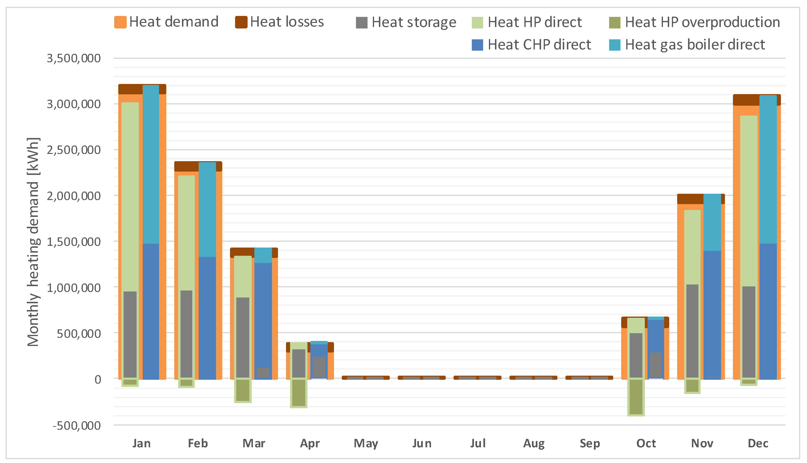
Figure 11 shows the monthly heat demand of Walheim (orange, in background) and how this demand is met by either the HP or CHP production and the storage (in front). On the left, the HP system plus storage is visualized in green, on the right in blue is the CHP and gas boilers plus storage. The CHP system always meets 100% of the demand, while the HP system has both under- and overproduction for most of the months. Overproduction for the HP occurs, when the storage tank is “full”, but the HP is still running for the remainder of the time step of one hour. This amount of energy is usable in reality, but leads to higher storage losses due to the temperature increase. This effect is due to the modeling time step of one hour. The storage (gray) is used in both systems, however the CHP unit can only produce significant surplus heat for storage in March, April, and October, when the monthly heat demand is considerately below 2000 MWh. In the summer months (May–September), the heating network is switched off, therefore only the storage losses remain.
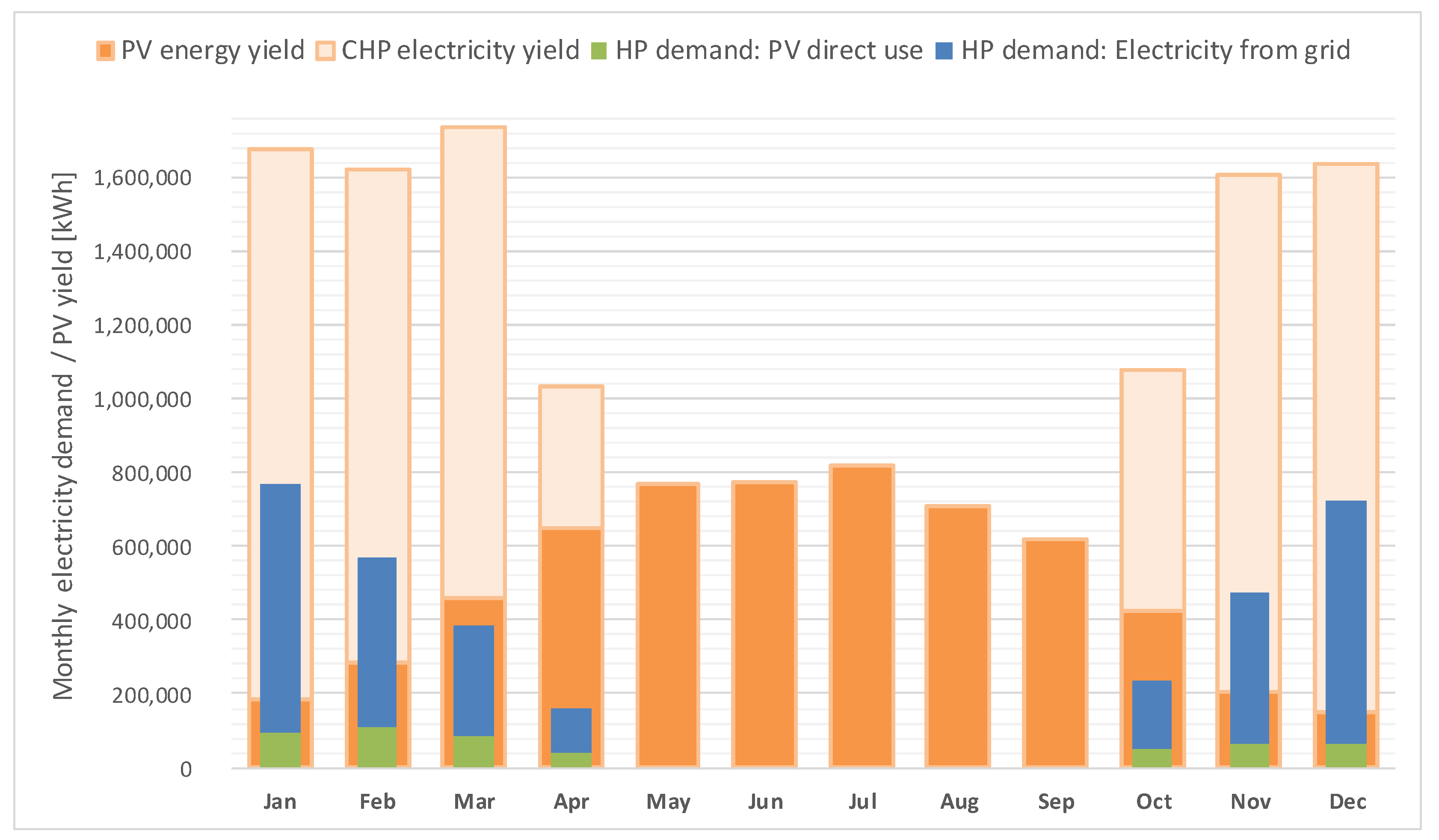
Both systems (HP and CHP scenario) generate the same amount of electricity with PV and the CHP system has additional electricity generation on top of the PV yield. The HP uses the PV electricity whenever possible. 15% of the HP electricity demand can thus be met by PV directly. Because of non-simultaneity, the rest of the electricity needed for the operation of the HP needs to come from the grid and 92% of the PV generated electricity is fed to the grid. This excludes the household electricity demand, which is the same in both scenarios and not taken into account here. Own-consumption of the PV electricity for household electricity demand is not assessed in this study.
The monthly comparison between the PV energy yield, the PV energy use by the HP and the remaining electricity needed from the grid for the operation of the HP can be seen in
Figure 12. It shows a mismatch of a high PV energy yield (orange) in the summer months and a high HP electricity demand (green plus blue) in the winter months. However, the annual electricity balance of HP demand and PV generation in the town of Walheim is positive (PV electricity yield is 82% higher than the HP electricity demand, see
Table 2).
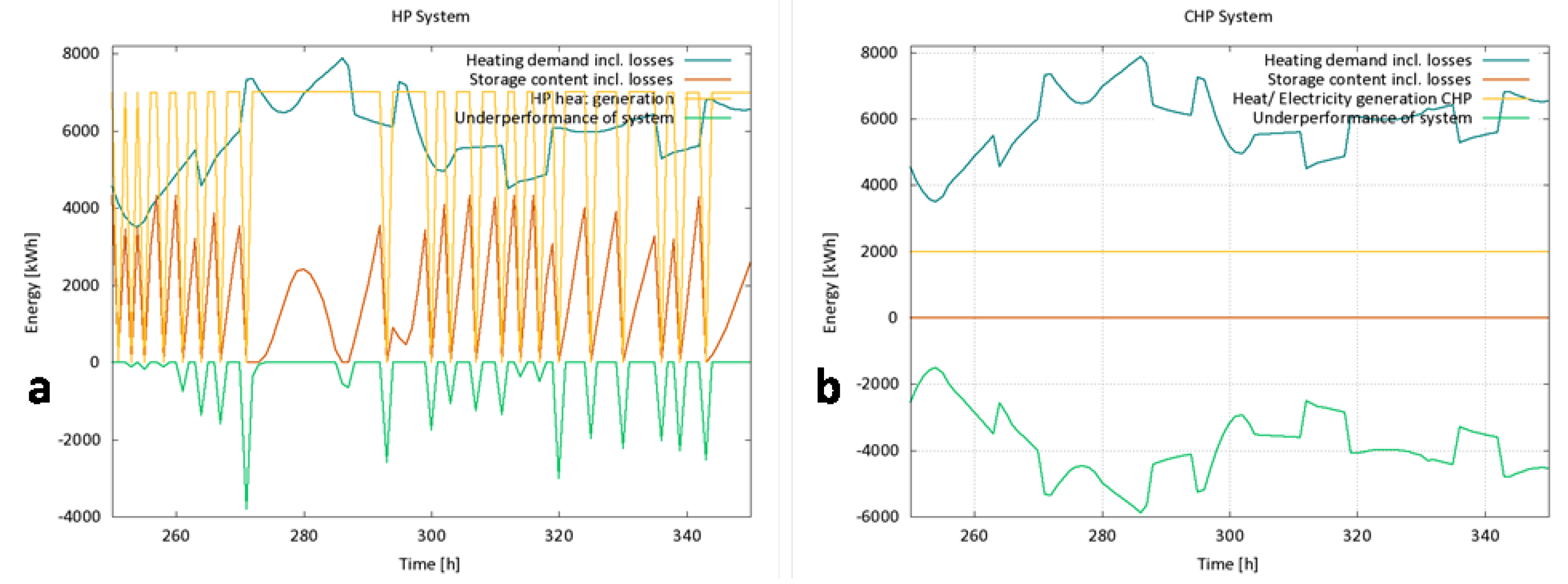
A period of 100 h in January is chosen to highlight the differences in heat generation and other KPIs for both systems (see
Figure 13). In this period, the heat demand reaches its peak with a load of 7767 kW. In
Figure 13 the modulation of the HP is clearly visible. The loads during hours 281 till 287 cannot be met by the HP directly. In most of those hours however, the demand can be met with heat from the storage, only for three hours the system does not produce enough heat. If the heat demand is lower than what the HP produces (e.g., in the first 10 h of the graph), the surplus heat fills the storage. This stored heat is then used to satisfy the heat demand when the HP turns off. However, when the HP is switched off and the demand is higher than the heat that is available in storage, there is a slight underperformance of the system. The deficit is only during one hour at a time and only once for two consecutive hours. The one-hour deficits are due to the model time step of one hour and do not have practical relevance, as the HP would switch on directly if the storage tank is below the threshold. This fact combined with the low-energy standard of the buildings and their surface heating system leads to the conclusion that this deficit is acceptable.
Figure 13b shows the same time period for the CHP system. The CHP unit runs constantly but can only provide part of the heat demand. This is due to the dimensioning of the CHP unit; the rest of the demand is provided by the gas boilers (not in the figure). The storage is empty since there is no surplus heat from the CHP available.
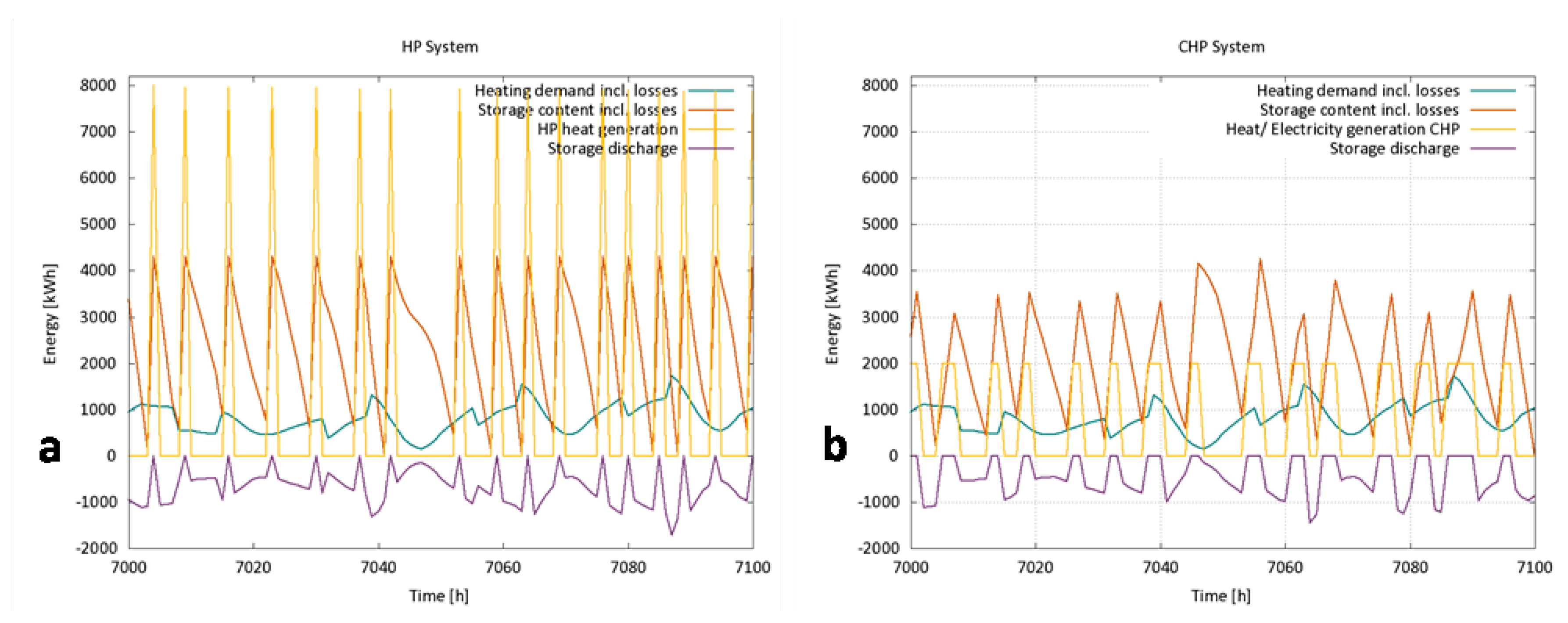
In
Figure 14, 100 h in mid-October are shown for both systems. In this period, the heat demand is lower than in
Figure 13, therefore the systems run differently.
Figure 11a shows that the HP system runs only one hour at a time, before switching off for four or more consecutive hours when the heat demand is met from the storage. Since the power of the CHP unit is lower than of the HP, less heat can be loaded into the storage in
Figure 14b compared to the HP system. Also, the CHP unit must run for more than one hour at a time and is switched off for only three to four consecutive hours.
6. Assessment of Primary Energy Demand
The primary energy demand is calculated by multiplying the final energy demand with a PEF that takes into account the effort and losses that occur during the whole value chain of the energy carrier.
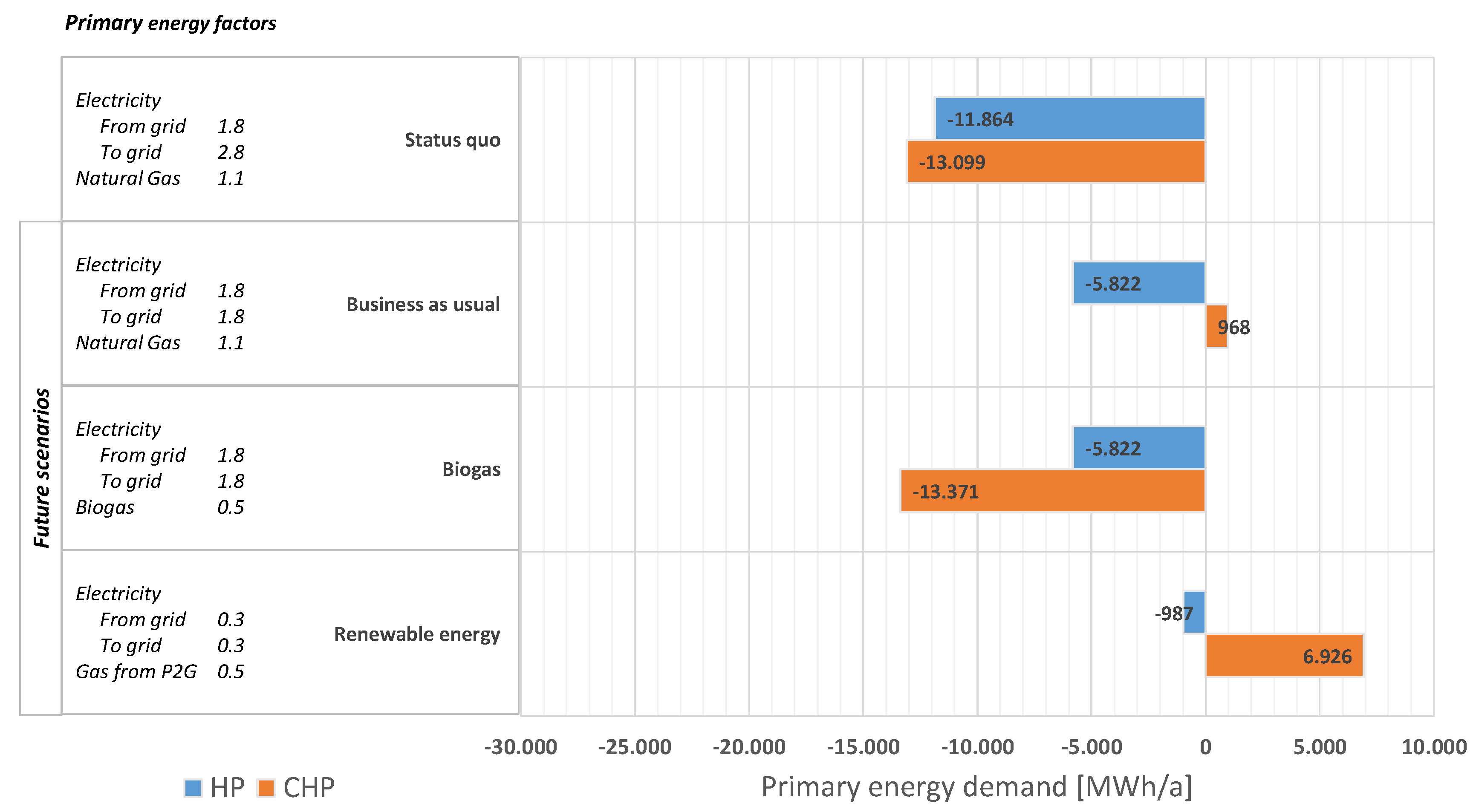
To demonstrate the influence of the energy carrier used as well as the influence of the current and future grid mix, different scenarios are calculated in
Figure 15. The electricity generated by the CHP unit can be assessed in different ways, depending e.g., on how the electricity in the grid is produced and what type of gas is used. If the CHP runs on natural gas and the electricity from the CHP and PV is fed into a grid with predominantly fossil and nuclear electricity generation, it replaces this kind of electricity with renewable or co-generated electricity. The current factor in Germany for this replacement is 2.8 [
56], which means that the electricity generated by the CHP and PV that is fed into this grid is valued 2.8 times higher than its actual amount of electricity (
Figure 15—status quo). Since the CHP units produce more electricity than the HP, the overall balance of the CHP is better. However, when the electricity mix of the grid changes in the future due to the integration of increasingly renewable electricity (
Figure 15—business as usual), this factor will have to change as well. Then, the surplus electricity would be worth less and the HP scenario wins against the CHP. If biogas is used in the CHP, the PEF for gas changes to 0.5. In this scenario (
Figure 15—biogas) the CHP has the better primary energy balance. According to a meta-study by the Ökoinstitut and Fraunhofer ISI [
57], the PEF for electricity in 2050 in Germany will be 0.3. Assuming an overall efficiency of 0.65 for the P2G process, this results in a PEF of 0.5 for gas from P2G (
Figure 15—renewable energy). In this case, the primary energy balance for the HP system is the better one, because the P2G process is subject to high energy losses and the electricity fed into the grid by the CHP is not able to replace any fossil fuels anymore.
In general, the use of PEF to compare different energy systems must be evaluated. With a growing share of renewable electricity that factor loses its validity and might have to be replaced by different indicators [
58].
7. Conclusions and Outlook
In this study, two renewable energy generation models are developed and applied to a small German town. The SimStadt simulation environment was extended to include the developed models for a central HP system with a district heating network and central storage as well as a CHP system with a district heating network and central storage. The investigated indicators include the heat demand and heat production as well as the electricity generation and electricity demand of the respective systems.
A HP scenario with PV has the main disadvantage that due to low winter irradiance, the fraction of PV electricity used directly by the HP is only 15%. The main share of PV electricity is produced in summer; the main share of heat demand however occurs in winter.
For the CHP energy generation, it is important to include the source of the gas used. If we assume renewable energy for all energy sources (renewable electricity for the HP system and either biogas or gas from P2G, produced from renewable electricity for the CHP system), a look at the total electricity needed for operation of the systems is essential.
To achieve a good match between demand and generation, it is important that energy generation from other renewable sources, such as wind, is investigated and further models and scenarios are created for the simulation environment. Additionally, different storage management schemes or storage types need to be investigated to maximize the usage of PV electricity by the HP.
In a next step, an economic analysis of the systems in question with their respective energy in- and outputs will be made. With this additional assessment, more KPIs for each system can be assessed and the systems can be compared on a broader level. At present, both HP and CHP system cannot regulate their heating power, so they are either running on full load or are switched off. Models that support partial load operation are under development right now and could provide a more detailed assessment and comparison of the two systems.
In conclusion, urban energy simulations are a very important instrument for analyzing demands and potentials and comparing different scenarios. Based on the simulation results, the overall energy efficiency can be improved, and emissions reduced. The outcome of these simulations can be used to advise city planners, building authorities or municipalities to help design a renewable and sustainable urban future.


