Historical Load Balance in Distribution Systems Using the Branch and Bound Algorithm

Abstract

One of the biggest problems with distribution systems correspond to the load unbalance created by power demand of customers. This becomes a difficult task to solve with conventional methods. Therefore, this paper uses integer linear programming and Branch and Bound algorithm to balance the loads in the three phases of the distribution system, employing stored data of power demand. Results show that the method helps to decrease the unbalance factor in more than 10%, by selecting the phase where a load should be connected. The solution may be used as a planning tool in distribution systems applied to installations with systems for measuring power consumption in different time intervals. Furthermore, in conjunction with communications and processing technologies, the solution could be useful to implement with a smart grid.

1. Introduction

Nowadays, modern distribution systems must support the continuous growing and variability of power demand, because of acquisition of new technologies and consumption habits of electrical appliances such as air conditioning systems, television sets, and washing machines. Although, a balanced distribution system is preferable with similar power in phases, these variable consumption behaviors lead to undesirable unbalance through the distribution system. Therefore, power balance helps to reduce technical losses and improve the use of resources such as capacitor banks and transformers load tap changers.

Distribution systems have more users than transmission systems, thus, measuring the consumption and performing load balancing become complex procedures [1]. Consequently, phase-load balancing methods for distribution systems employed in utility companies use nominal loads and diversity factors, assuming power consumption does not change considerably. Hence, electricity providers use theoretical information on regular operating conditions and contingencies.

According to Quintela et al. [2], load balancing in distribution systems is seldom employed as technical habit to improve regulation losses. However, there are different proposals to decrease losses in electrical systems using linear programming techniques. Franco et al. [3] used these tools to solve the problem of conductor size selection (CSS) in radial distribution systems. Baran and Wu [4] studied algorithms for reconfiguration in medium voltage (MV) systems, requiring three-phase switches. Olamaei et al. also studied feeder reconfiguration in distribution systems, using Particle Swarm Optimization (PSO) [5]. A different approach uses linear and non-linear programming techniques for reconfiguration in distribution systems [6].

On the other hand, load balance tries to obtain the same amount of current in each phase. To achieve this balance, the studies in references [7,8,9,10] employed additional components in the network, such as electric springs, a phase balancer, and reactive power compensating devices. A different approach, known as phase swapping, assigns loads to every phase in the system, in order to obtain a similar current in each phase. There are different algorithms proposed to achieve balance through phase swapping: One example tested two methods: Fuzzy Simulated Annealing (FSA) and Fuzzy Evolutionary Particle Swarm Optimization (FEPSO), to balance a real low voltage system from Argentina [11]. Zdraveski et al. [12] presented a dynamic, intelligent load balancing (DILB) algorithm for selecting the phase where each load should be connected. The paper suggests employing a rotary switch for load connection. A different study proposed a self-adaptive hybrid differential evolution (SaHDE) algorithm, tested in modified IEEE 34 and IEEE 123 node systems [13]. Another paper used genetic algorithms to achieve load balance through simulations of a real system from Iran [14]. Singh et al. investigated particle swarm optimization for load balance. Zhu, Chow, and Zhang employed mixed integer programming with Branch and Bound (B&B) algorithm [15]. However, all these studies compute balance for one specific time. For balancing in long-term conditions (that is, through different intervals), all algorithms must run continuously, possibly modifying load connections to each phase in every period considered for analysis.

Ballesteros and Souza [16] showed that research to decrease power losses in primary distribution systems is vast, but not as much in secondary systems. The authors tested five algorithms to balance secondary networks. All algorithms create different connection matrices showing what phase each load should be connected to, and the method chose the one with fewer switching operations to perform instant balancing. Another study used a modified Leapfrog algorithm, in order to maintain the position of the switches during different periods to achieve load balance. The study simulated 10 loads during 24 h and three different scenarios, reducing network unbalance [17]. A different study used Petri nets to encompass different algorithms as follows: Fuzzy inference to identify load unbalance and to perform load transfer between phases or feeders, Markov chains to forecast the load consumption, and switch selection based on an optimal choice algorithm [18].

This paper presents a load balancing procedure using optimization and linear programming techniques with B&B for one feeder, and a node or distribution transformer based upon customer power consumption during different periods. Hence, the algorithm may be used in Smart Grids with systems for measuring such data. The main contributions of this paper are:

• Unlike other works, this method employs historical data to achieve load balance by swapping each load to a phase that is fixed throughout the analysis time and no additional switching operations are required. This fact is important because switching is one cause of transient disturbances [19].
• Additionally, the method finds a way to establish the historical load balance by using an unbalance factor on each phase for every time. The unbalance factor of the system is the maximum value of unbalance in all three phases during the analysis time, allowing quantification of the improvement obtained with the proposed solution.
• Historical load configurations may create unfeasible balance problems; however, the proposed method uses different load percentages on each phase to minimize the chance of unfeasible solutions and finds the optimal solution using B&B, which may not be guaranteed with heuristic methods.

The paper is organized as follows: Section 2 defines the research problem. Section 3 presents the proposed solution for load balancing using B&B. Section 4 shows simulation results. Section 5 concludes the paper.

2. Problem Formulation

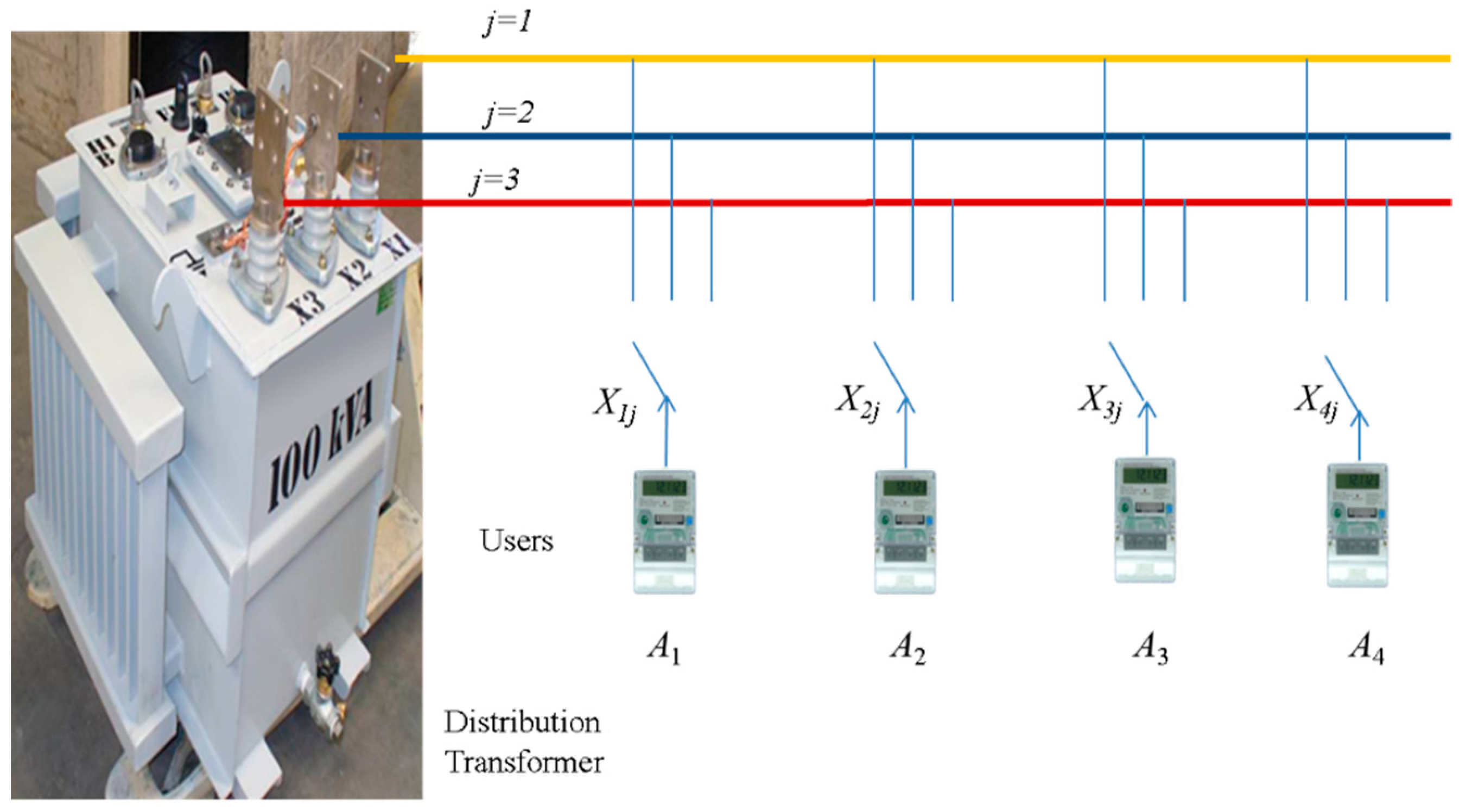
Customers in an electric distribution system connect to one or more phases of a node, such as a transformer. The method assumes only single-phase loads connected to the distribution node and every customer load has a specific value (demand), which depends only upon the customer profile. For example, Figure 1 shows four customers that may be connected to one of the j phases of the distribution node.

The total active power consumption B in a distribution node is the summation of all individual loads connected to the node. If every customer i has total active power A_i, the following equation shows total power consumption for n customers:

$$A_1+A_2+A_3+\cdots +A_n={\displaystyle \sum }_{i=1}^n{A}_i=B.$$

(1)

Additionally, total active power is the summation of the active power of each phase, B_j, as presented in Equation (2):

$$B_1+B_2+B_3={\displaystyle \sum }_{j=1}^3{B}_j=B.$$

(2)

The proposed solution includes switches for connecting each customer to one specific phase. X_ij is the switch state of load A_i in phase j. Therefore, Equation (3) shows the total active power on each phase:

$$\begin{array}{c}{A}_1{X}_{11}+A_2{X}_{21}+A_3{X}_{31}+\cdots +A_n{X}_{n1}=B_1,\\ A_1{X}_{12}+A_2{X}_{22}+A_3{X}_{32}+\cdots +A_n{X}_{n2}=B_2,\\ A_1{X}_{13}+A_2{X}_{23}+A_3{X}_{33}+\cdots +A_n{X}_{n3}=B_3,\end{array}$$

(3)

where A_i is the power load demand of each customer i, B_j is total active power per phase, index j ∈ {1, 2, 3} represents the phase and X_ij is the switch state of load A_i in phase j, represented with a binary variable:

$$X_{ij}\in \left\{0,1\right\},$$

(4)

where 1 indicates connection and 0 indicates disconnection of the specific load. Additionally, each switch connects one load exclusively to one phase, as presented in Equation (5):

$${\displaystyle \sum }_{j=1}^3{X}_{ij}=1.$$

(5)

Each phase feeds a portion of the total demand at every moment. Equations (6) and (7) present this situation for a three-phase distribution node:

$$\begin{array}{c}{B}_1={\lambda }_{1}B,\\ B_2={\lambda }_{2}B,\\ B_3={\lambda }_{3}B,\end{array}$$

(6)

$${\displaystyle \sum }_{j=1}^3{\lambda }_j=1,$$

(7)

where λ_j is the fraction of the total demand supplied by phase j. In a perfectly balanced node, λ₁ = λ₂ = λ₃ = 1/3 for each period. However, in practice the real values of λ_j are different for each time and phase.

Note the equations apply to only one interval. Long-term load balance requires performing the computation for different time intervals and obtaining the best switch configuration. Equation (8) shows the total power of phase 1 represented by B_k1 in each period k (for k = 1 to m periods); herein, A_ki represents the loads in the period k of customer i (for i = 1 to n customers) and X_kij is the connection of customer i to phase j in period k:

$$\begin{array}{cc}{A}_{11}{X}_{111}+A_{12}{X}_{121}+\cdots +A_{1n}{X}_{1n1}& =B_{11},\\ A_{21}{X}_{211}+A_{22}{X}_{221}+\cdots +A_{2n}{X}_{2n1}& =B_{21},\\ ⋮& \\ A_{m1}{X}_{m11}+A_{m2}{X}_{m21}+\cdots +A_{mn}{X}_{mn1}& =B_{m1}.\end{array}$$

(8)

In general, the power demanded to phase j in period k can be expressed as:

$$\begin{array}{cc}{\displaystyle \sum _{i=1}^n}{A}_{ki}{X}_{kij}=B_{kj},& j,k\in \mathbb{N}, 1\le j\le 3, 1\le k\le m.\end{array}$$

(9)

The general expression allows switching every load to every phase at every time interval, which is possible in smart grids. However, periodic switching produces transient disturbances that degrade the quality of the provided energy [19]. The goal of this paper is to develop a method capable of balancing the loads using the same connections during all the periods. Therefore, the connection vectors are restricted by Equation (10). Note that the load A_ki of customer i will be connected to (or disconnected from) phase j during all m periods.

$$X_{1ij}=X_{2ij}=\cdots =X_{mij}=X_{ij}.$$

(10)

The objective function to be maximized is the sum of the binary variables X_ij for all the n customers in phase j. The objective function is restricted by the power balance of each phase. The restrictions enforce the objective function to converge to a connection vector representing a fraction of the total demand as close as possible to the fraction defined in Equation (6).

The optimization problem for phase j can be expressed as:

$$\underset{{\overrightarrow{X}}_j}{\max }f\left({\overrightarrow{X}}_j\right)={\displaystyle \sum }_{i=1}^n{X}_{ij},$$

(11)

subject to:

$$\begin{array}{cc}{\displaystyle \sum _{i=1}^n}{A}_{ki}{X}_{ij}=B_{kj}\le {\lambda }_j{B}_k,& \forall k\in \mathbb{N},1\le k\le m,\end{array}$$

(12)

where:

• X_ij: Binary variable showing connection (1) or not (0) of load i to phase j during all periods.
• ${\overrightarrow{X}}_j$: Connection vector of phase j, defined as [X_1j, X_2j, …, X_nj]^T.
• A_ki: Active power from load (customer) i in time k.
• B_k: Available capacity in time k, namely the total power delivered to customers in that specific period.
• λ_j: Maximum percentage of the total power supplied by phase j during all periods.
• n: Number of loads in the system.
• m: Number of time periods.

Note that Equation (12) shows the situation in each phase, since λ_jB_k corresponds to the percentage of total power assigned to one phase. These equations fulfill the power boundaries for each phase in each given period and during the whole analysis time. Most related studies perform load balance in one given interval. On the other hand, the objective in this work is to obtain the better balance during the whole time of analysis. The proposed solution uses customer profiles in different periods to achieve the best load distribution possible in all available phases.

To determine an objective metric for load balance, the method employs the relation between the total active power in one period, B_k, and the power of each phase in that period B_kj. Equation (13) presents the unbalance factor of phase j for period k (UF_kj), to compute an error ratio for a three-phase system:

$$U{F}_{kj}=\left|\frac{1}{3}-\frac{B_{kj}}{B_k}\right|$$

(13)

Equation (13) assumes that 1/3 is the reference value for the ideal balance in a three-phase system, since the total load should be equally split between all three phases. According to Equation (13), the unbalance factor changes during each period k and each phase j. Thus, Equation (14) defines the unbalance factor of the system UF_s as the maximum unbalance factor of the distribution system, obtained as the maximum of all unbalance factor values UF_kj of all k periods and j phases. Note that UF_s shows the worst case of load balance for all phases and periods.

$$U{F}_s=\underset{k,j}{\max }U{F}_{kj}$$

(14)

3. Proposed Solution

Figure 2 shows a summary of the proposed method that will be explained in each of the following subsections.

The proposed method computes an initial value of UF_s for the unbalanced distribution system, to compare it to the final solution. The expected solution is the connection matrix including the position of all switches X_ij, where each load must be connected to a phase, and UF_s decreases compared to the unbalanced distribution system. Since the method computes the initial value of UF_s and this value depends upon the loads and periods, the method should run every time new loads are installed in the system.

3.1. Definition of λ_j

Using all demand values, the algorithm computes B and defines λ_j values to distribute the loads similarly in each phase. The process has different stages; the first stage defines λ₀, which is the sum of initial λ values for phases 1 and 2 (λ₁₀ and λ₂₀). Ideally, λ₀ should be 2/3 and λ₂₀ should be 1/3, because power in each phase should be one third of the total. However, λ values are not fixed because customer load values cannot be changed. Therefore, it is not likely that every phase has exactly one third of the total load. Hence, the method explores different λ values in subsequent stages.

3.2. Use Branch and Bound to Obtain X_ij

After defining λ_j, the method employs the B&B algorithm [20] to determine what phase each load should be connected to. The resulting solution shows the values of X_ij, known as the connection matrix. The algorithm can be described as a search of the optimum value over the feasible region by dividing (branching) the region into smaller areas, discarding unfeasible areas and repeating the process over the remaining areas. The algorithm stops when there are no more nodes in the search tree to be branched and all the nodes have been bounded. The solution of the problem is the current best solution at the moment the algorithm stops. If B&B terminates properly (it does not stop early), it ensures global optimality of the solution found. If B&B terminates properly without finding a solution, then the original problem itself is unfeasible [21]. Therefore, the proposed method has two different outcomes: The first one is that problem is unfeasible: No X_ij values can fulfill all restrictions with current λ values; and the second one is that B&B finds X_ij values that satisfy the restrictions and the solution may exhibit a better balance than the original configuration.

The two outcomes depend upon λ values. In the first case, it is mandatory to modify λ values, in order to find adequate solutions. The second case already presents a balanced system and the method computes a new UF_s to compare the balanced solution to the initial value. If the new UF_s in the solution is smaller than the initial UF_s, the solution becomes a candidate for load balance. Otherwise, a new calculation is required.

3.3. Modification of λ Values

After finding a candidate solution, the method increases the initial λ₂₀ value in steps of Δλ₂, up to a maximum established value (λ_2f). After this value, if the process finds no solutions, the algorithm increases λ₀ in Δλ₀ up to a maximum value (λ_0f) and λ₂ starts in λ₂₀ again. If the procedure finds a solution, it stores the connection matrix, computes UF_s and continues looking for a better solution by increasing λ₁ and λ₂ as previously described. This procedure decreases the possibility of finding unfeasible solutions.

The algorithm ends when all λ_j reach the maximum established values. The final solution includes X_ij values and the final UF_s that can be compared to the initial UF_s to determine balance improvement in the network.

Note all calculations depend upon load and period values, therefore, the solution may vary if historical data includes different analysis periods. However, the method always computes UF_s, the worst case of load balance for all phases and periods, finding a solution to improve this metric.

4. Results

4.1. Test Case

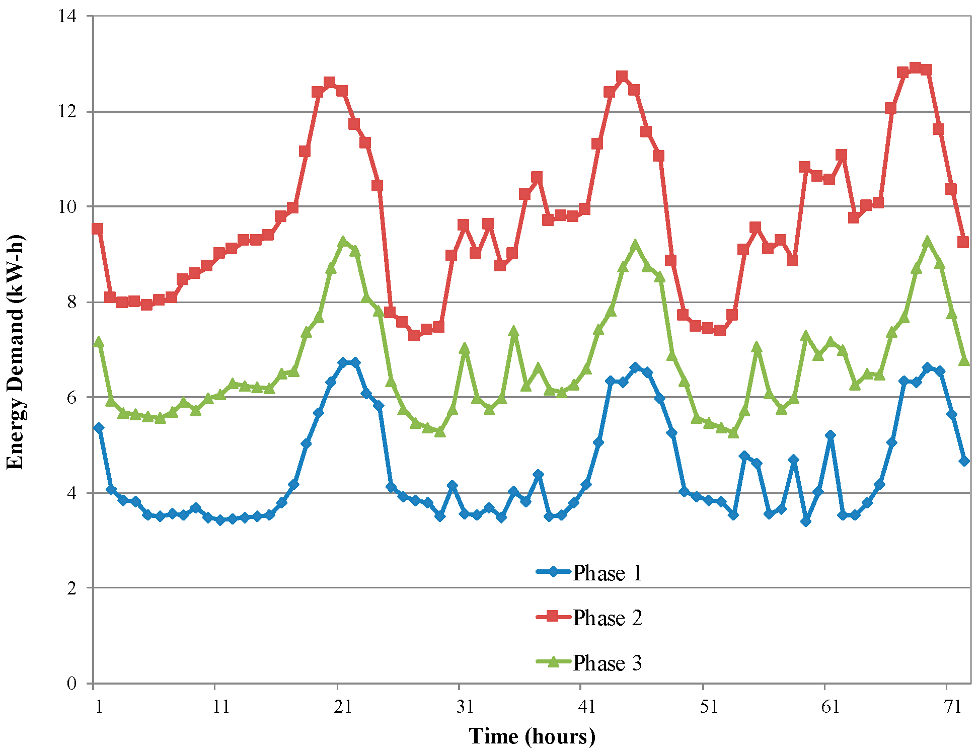
This section presents one application of the method to visualize the performance of the algorithm. The method was tested with data for hourly demands in 72 periods of time and 10 single-phase loads connected to a three-phase system, as in reference [19]. Thus,

Table 1. Connection matrix for the three-phase distribution system with 10 single-phase loads [19].

Phase	Load
	1	2	3	4	5	6	7	8	9	10
1	0	1	0	0	1	0	0	0	0	0
2	1	0	0	1	0	0	1	1	0	1
3	0	0	1	0	0	1	0	0	1	0

presents the initial connection matrix, where the number “1” means connection and the number “0” means disconnection.

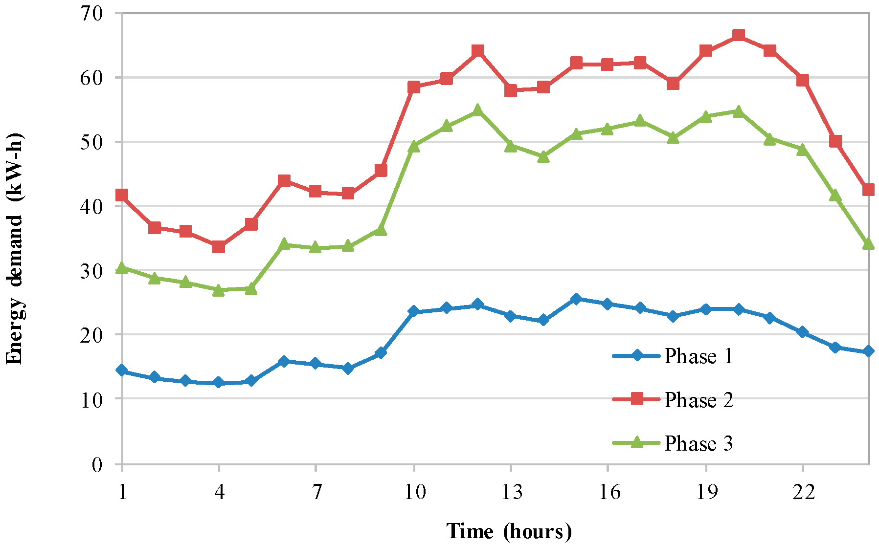
Figure 3 shows the behavior in time for the different phases for the example demands from reference [19]. The power demanded during the day is used to simulate the scenarios from the initial connection.

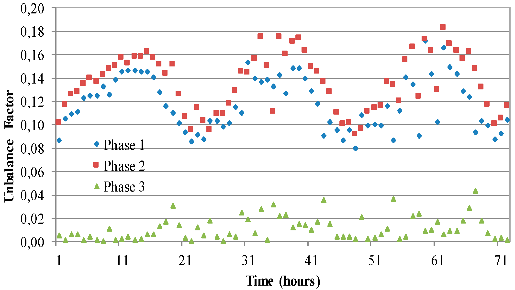
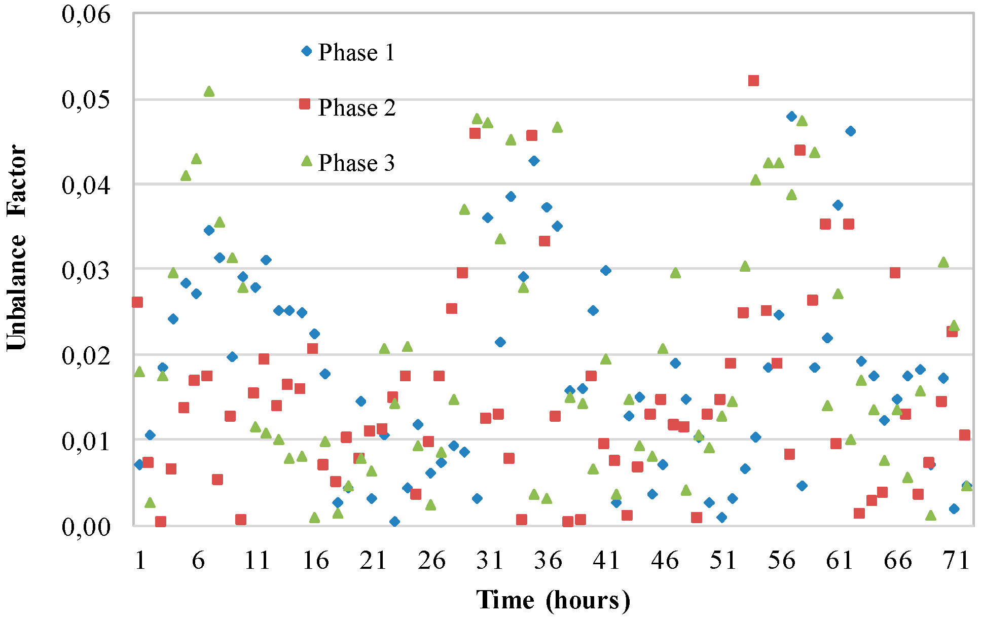
The first step in our method is computing the initial value of UF_s. Figure 4 shows all values of UF_ij for all phases in the system. According to the figure, the maximum values obtained are 0.172, 0.183, and 0.043 for phases 1, 2, and 3, respectively. Therefore, the maximum value for the system with the initial configuration (UF_s0) is 0.183.

The next steps are to assign λ_j values and to use B&B to find a candidate load balance solution and to compute UF_s for this solution.

Table 2. Unbalance factors computed per phase for the example in Figure 3, with different λ values using the proposed method.

λj		Maximum Unbalance Factor Per Phase			UFs
0	2	Phase 1	Phase 2	Phase 3
0.71	0.46	0.120	0.085	0.115	0.120
0.71	0.49	0.108	0.147	0.115	0.147
0.72	0.43	0.076	0.092	0.051	0.092
0.72	0.50	0.061	0.085	0.051	0.085
0.72	0.51	0.048	0.052	0.051	0.052

shows different options with maximum UF_ij values computed for each phase.

The last column in Table 2 shows the maximum value for the system, UF_s. Then, the proposed method selects the last option in Table 2 as the best load balance configuration, since the combination of λ values (0.72 and 0.51) and the application of B&B generate 0.052 as the minimum of all UF_s values. Therefore, the selected solution achieves a maximum unbalance of 5.2% in all phases during the whole analysis time.

Table 3. Final three-phase connection matrix X_ij for load balance with proposed algorithm, corresponding to Figure 4.

PHASE	Load
	1	2	3	4	5	6	7	8	9	10
1	0	0	0	1	0	1	0	0	1	0
2	1	0	0	0	1	0	1	1	0	1
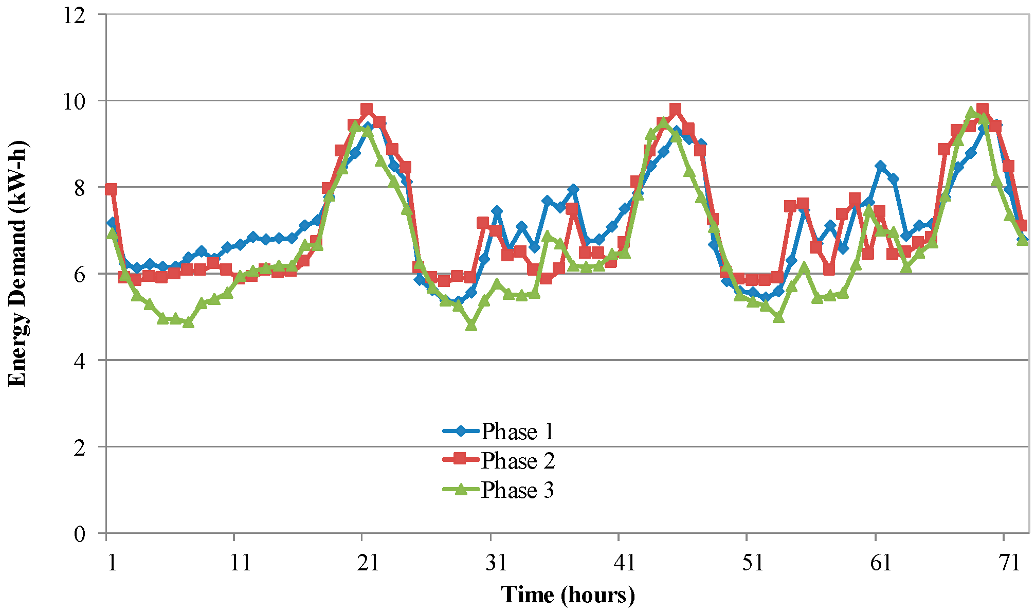
3	0	1	1	0	0	0	0	0	0	0

shows the connection matrix for the best balance solution, yielding results in Figure 5. Note all connections remain the same during the 72 periods.

Comparing the final UF_s (0.052) with the initial UF_s (0.183), improvement is 13.1%. Network operators may use this value to determine if they should implement the proposed load balance or not.

To verify UF conditions at all times, Figure 6 shows UF_ij values for every phase and each one of the periods using the connections proposed in Table 3. Note that UF_ij values are consistent with Table 2, where UF_s is 0.052. Additionally, most of the time UF_ij values are below 0.03, showing a better balance. However, UF_s is a metric of the worst case of balance during the analysis time. Furthermore, Figure 6 also corresponds to Figure 5, since power of each phase is similar to each other, therefore, the unbalance factor is expected to be small.

4.2. Test on a Real Distribution System

The last test shows the effectiveness of the method by balancing the loads of a real low voltage (LV) system in the city of Bariloche, Argentina. The system corresponds to one of the six outputs of a medium and low voltage substation [10]. The original system has 10 feeders with 115 loads. To adapt the system to only one feeder, we reduced all feeders except the main one to a single-phase load, corresponding to the sum of the balanced loads of the feeder. The reduced system has 51 loads. Figure 7 shows the reduced feeder with each load connected the same way as in the actual system [10].

The average power demand per user of each load is presented in

Table 4. Test system average demand per load, per user (p.u.) [10].

Load #	Av. Demand (p.u.)	Load #	Av. Demand (p.u.)	Load #	Av. Demand (p.u.)
1	1.530	18	0.978	35	0.978
2	0.978	19	0.978	36	0.995
3	0.978	20	0.978	37	0.978
4	1.658	21	0.978	38	1.003
5	0.978	22	0.995	39	1.156
6	0.978	23	0.986	40	1.156
7	0.961	24	0.978	41	1.156
8	0.969	25	0.961	42	1.156
9	0.978	26	0.961	43	5.763
10	0.978	27	0.952	44	6.713
11	0.969	28	0.961	45	9.442
12	0.978	29	0.978	46	5.597
13	2.491	30	0.978	47	10.287
14	0.952	31	0.978	48	10.506
15	0.961	32	1.003	49	3.737
16	0.850	33	0.986	50	10.838
17	0.978	34	0.978	51	6.205

. These demands were calculated by taking the apparent power of the loads, given in reference [10], and assuming a power factor of 0.85. Data presented in [10] does not include customer load variation with time, thus a more realistic load profile of the customer was generated by classifying the loads into three categories: Residential, industrial, and atypical. Each load profile includes 24 h with steps of 1 h using a base load curve depending on the load category. The average of the load profile is the same as the value of the original static load in reference [10]. Most of the loads in the system are residential, because the substation is located in a suburban area.

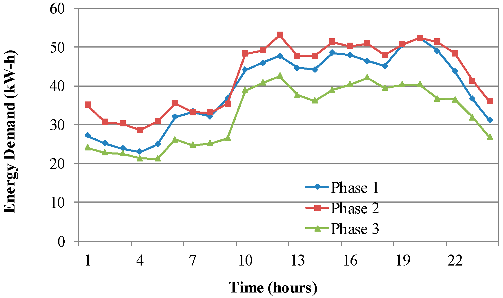
Figure 8 shows the initial demand profiles for each phase. Note that the initial load profile is obtained from the load connections shown in Figure 7, which correspond to the physical connections of the actual system.

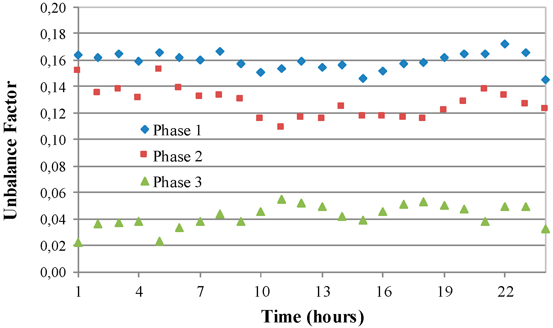
Figure 9 shows the unbalance factor in each period for all three phases. Maximum values are 0.17 in Phase 1, 0.154 in Phase 2, and 0.056 in Phase 3. Therefore, UF_s is 0.17.

With this information, we applied the proposed method to obtain a better balance solution.

Table 5. Connections for the Bariloche feeder, using the proposed method.

Load #	Phase	Load #	Phase	Load #	Phase
1	1	18	2	35	3
2	2	19	2	36	2
3	2	20	2	37	2
4	2	21	2	38	3
5	2	22	3	39	2
6	3	23	2	40	3
7	2	24	3	41	3
8	2	25	3	42	3
9	2	26	3	43	1
10	2	27	1	44	2
11	3	28	2	45	3
12	2	29	3	46	1
13	2	30	2	47	2
14	3	31	1	48	3
15	2	32	2	49	1
16	3	33	1	50	2
17	3	34	3	51	3

shows the connections obtained with the proposed method. Recall, every load connects to only one phase during the whole analysis time.

Figure 10 shows the resulting demands for each phase using the proposed method and the connections from Table 5. Comparing the initial situation in Figure 8 with the proposed solution, Figure 10 shows a better balance between the loads. However, it is important to quantify the amount of balance achieved with the method.

Figure 11 shows the unbalance factor during all analysis time. Maximum value for Phase 1 is 0.043, Phase 2 is 0.076, and Phase 3 is 0.062, therefore, UF_s after load balance is 0.076, a reduction of 9.4% from the original system. Additionally, Figure 11 shows UF values decreased in Phases 1 and 2, making these values similar for all phases and supporting the benefits of the proposed system.

5. Conclusions

The research presented in this paper provides a tool for historical load balance by suggesting appropriate connections to each one of the phases, employing data of customer power demand in different periods. The proposed method does not require switching during the analysis time and creates a solution for a total given time; therefore, the algorithm does not affect power quality of the distribution system. Additionally, the method uses different load percentages on each phase to minimize the chance of unfeasible solutions and finds optimal load balance with Branch and Bound. The method was tested with example data and with information from a real LV system, decreasing the unbalance factor of the system by 10%, as confirmed by the maximum unbalance value in all three phases during the analysis time. The solution may be used as a planning tool in distribution systems applied to installations with systems for measuring power consumption in different time intervals. The method may be implemented locally in each node, either with manual actions or automatically with Smart Grid functionality.

Future research should test the proposed method in the field using distribution transformers located in urban neighborhoods to identify advantages and disadvantages of the implementation and suggest possible adjustments. Extended research should be performed for several nodes in a circuit and include additional electrical metrics.

References

- See, J.; Carr, W.; Collier, S.E. Real Time Distribution Analysis for Electric Utilities. In Proceedings of the 2008 IEEE Rural Electric Power Conference, Charleston, SC, USA, 27–29 April 2008; pp. B5-1–B5-8. [Google Scholar] [CrossRef]
- Quintela, F.R.; Arévalo, J.M.G.; Melchor Redondo, N. Desequilibrio y pérdidas en las instalaciones eléctricas. Montajes e Instala. 2000, 338, 77–82. [Google Scholar]
- Franco, J.F.; Rider, M.J.; Lavorato, M.; Romero, R. Optimal Conductor Size Selection and Reconductoring in Radial Distribution Systems Using a Mixed-Integer LP Approach. IEEE Trans. Power Syst. 2013, 28, 10–20. [Google Scholar] [CrossRef]
- Baran, M.E.; Wu, F.F. Network reconfiguration in distribution systems for loss reduction and load balancing. Power Deliv. IEEE Trans. 1989, 4, 1401–1407. [Google Scholar] [CrossRef]
- Olamaei, J.; Niknam, T.; Gharehpetian, G. Application of particle swarm optimization for distribution feeder reconfiguration considering distributed generators. Appl. Math. Comput. 2008, 201, 575–586. [Google Scholar] [CrossRef]
- Khodr, H.M.; Martinez-Crespo, J.; Matos, M.A.; Pereira, J. Distribution systems reconfiguration based on OPF using benders decomposition. IEEE Trans. Power Deliv. 2009, 24, 2166–2176. [Google Scholar] [CrossRef]
- Yan, S.; Tan, S.-C.; Lee, C.-K.; Chaudhuri, B.; Hui, S.Y.R. Electric Springs for Reducing Power Imbalance in Three-Phase Power Systems. IEEE Trans. Power Electron. 2015, 30, 3601–3609. [Google Scholar] [CrossRef] [Green Version]
- Gupta, N.; Swarnkar, A.; Niazi, K.R. A novel method for simultaneous phase balancing and mitigation of neutral current harmonics in secondary distribution systems. Int. J. Electr. Power Energy Syst. 2014, 55, 645–656. [Google Scholar] [CrossRef]
- Korovkin, N.V.; Vu, Q.S.; Yazenin, R.A. A method for minimization of unbalanced mode in three-phase power systems. In Proceedings of the 2016 IEEE NW Russia Young Researchers in Electrical and Electronic Engineering Conference (EIConRusNW), St. Petersburg, Russia, 2–3 February 2016; IEEE: Piscataway, NJ, USA, 2016; pp. 611–614. [Google Scholar]
- Yuvaraj, T.; Ravi, K.; Devabalaji, K.R. DSTATCOM allocation in distribution networks considering load variations using bat algorithm. Ain Shams Eng. J. 2017, 8, 391–403. [Google Scholar] [CrossRef] [Green Version]
- Schweickardt, G.; Alvarez, J.M.G.; Casanova, C. Metaheuristics approaches to solve combinatorial optimization problems in distribution power systems. An application to Phase Balancing in low voltage three-phase networks. Int. J. Electr. Power Energy Syst. 2016, 76, 1–10. [Google Scholar] [CrossRef]
- Zdraveski, V.; Todorovski, M.; Kocarev, L. Dynamic intelligent load balancing in power distribution networks. Int. J. Electr. Power Energy Syst. 2015, 73, 157–162. [Google Scholar] [CrossRef]
- Sathiskumar, M.; Nirmal kumar, A.; Lakshminarasimman, L.; Thiruvenkadam, S. A self adaptive hybrid differential evolution algorithm for phase balancing of unbalanced distribution system. Int. J. Electr. Power Energy Syst. 2012, 42, 91–97. [Google Scholar] [CrossRef]
- Najafi, A.; Dehghanian, M.; Attar, M.; Falaghi, H.; Homaee, O. A practical approach for distribution network load balancing by optimal re-phasing of single phase customers using discrete genetic algorithm. Int. Trans. Electr. Energy Syst. 2019, e2834. [Google Scholar] [CrossRef]
- Jinxiang Zhu, J.; Mo-Yuen Chow, M.-Y.; Fan Zhang, F. Phase balancing using mixed-integer programming [distribution feeders]. IEEE Trans. Power Syst. 1998, 13, 1487–1492. [Google Scholar] [CrossRef]
- Luis roberto, B.H.; Raimundo Cláudio, S.G. Balance de Cargas en Circuitos Secundarios de Distribución. Revista Científica de Ingeniería Electrónica, Automática y Comunicaciones 2011, 32, 21–34. [Google Scholar]
- Raminfard, A.; Shahrtash, S.M.; Herizchi, T.; Khoshkhoo, H. Long-Term Load Balancing Program in LV Distribution Networks. In Proceedings of the 2012 IEEE International Power Engineering and Optimization Conference Melaka, Malacca, Malaysia, 6–7 June 2012; Volume 1, pp. 6–7. [Google Scholar]
- Da Costa, C.; Oliveira, W.; Oliveira, R.; Silva, J.; Sicchar, J. A Load-Balance System Design of Microgrid Cluster Based on Hierarchical Petri Nets. Energies 2018, 11, 3245. [Google Scholar] [CrossRef]
- Stanek, M. Experiences with Improving Power Quality bye Controlled Switching. In Proceedings of the CIGRE WG A3.07: Seinar and Workshop on Controlled Switching, St. Pete Beach, FL, USA, 7 May 2003; pp. 1–5. [Google Scholar]
- Winston, W.L.; Goldberg, J.B. Operations Research: Applications and Algorithms; Duxbury Press: Belmont, CA, USA, 2004. [Google Scholar]
- Clausen, J. Branch and Bound Algorithms-Principles and Examples; Department of Computer Science, University of Copenhagen: Copenhagen, UK, 1999; pp. 1–30. [Google Scholar]
Figure 1.
Connection diagram for four loads in a distribution node for phases 1, 2, and 3. Xij are switches to connect each user to only one phase.
Figure 2.
Flowchart of the proposed method.
Figure 3.
Example hour demands for 10 single-phase loads in 72 h [19].
Figure 4.
Unbalance factor for each phase and period.
Figure 5.
Demand curves for the example in Figure 3 after load balance employing the proposed method.
Figure 7.
Reduced low voltage (LV) feeder system, adapted from reference [10].
Figure 8.
Initial demand curves for Bariloche, Argentina.
Figure 9.
Initial unbalance factors for all periods, Bariloche.
Figure 10.
Balanced demand curves for Bariloche, Argentina.
Figure 11.
Unbalance factor after applying the proposed method for Bariloche, Argentina.