Short-Term Photovoltaic Power Output Prediction Based on k-Fold Cross-Validation and an Ensemble Model

Electric Engineering College, Tibet Agriculture and Animal Husbandry University, Nyingchi 860000, Tibet Autonomous Region, China
*
Author to whom correspondence should be addressed.
Energies 2019, 12(7), 1220; https://0-doi-org.brum.beds.ac.uk/10.3390/en12071220
Submission received: 28 February 2019
/
Revised: 20 March 2019
/
Accepted: 25 March 2019
/
Published: 29 March 2019
(This article belongs to the Special Issue Solar and Wind Power and Energy Forecasting)
Abstract
:Short-term photovoltaic power forecasting is of great significance for improving the operation of power systems and increasing the penetration of photovoltaic power. To improve the accuracy of short-term photovoltaic power forecasting, an ensemble-model-based short-term photovoltaic power prediction method is proposed. Firstly, the quartile method is used to process raw data, and the Pearson coefficient method is utilized to assess multiple features affecting the short-term photovoltaic power output. Secondly, the structure of the ensemble model is constructed, and a k-fold cross-validation method is used to train the submodels. The prediction results of each submodel are merged. Finally, the validity of the proposed approach is verified using an actual data set from State Power Investment Corporation Limited. The simulation results show that the quartile method can find outliers which contributes to processing the raw data and improving the accuracy of the model. The k-fold cross-validation method can effectively improve the generalization ability of the model, and the ensemble model can achieve higher prediction accuracy than a single model.
1. Introduction
With the decrease of traditional fossil energy use, it has become the consensus of the world to develop renewable energy, such as photovoltaic energy, on a large scale. Between 1992 and 2018, there was a dramatic worldwide growth in the usage of photovoltaic power. During this period of time, photovoltaic (PV) energy, also known as solar PV, evolved from a niche market of small-scale applications to a mainstream electricity source. By the end of 2018, the cumulative photovoltaic capacity reached about 512 gigawatts (GW), estimated to be sufficient to supply 2.55% of the global electricity demand. However, photovoltaic power generation has the characteristics of fluctuation and intermittence, which brings new challenges to the safe operation of power systems [1]. Accurate prediction of the photovoltaic power output in the future has vital significance for improving the operation of power systems and increasing the penetration of photovoltaic power [2,3].
In recent years, experts and scholars have proposed many algorithms for short-term photovoltaic power prediction and have achieved remarkable results. The existing methods for photovoltaic power prediction can be summarized as statistical methods, physical methods, and machine learning methods. (1) Statistical methods mainly include time series methods [4], wavelet analysis [5,6], classification regression [7,8], and spectral analysis [9]. These methods use statistical principles to establish a functional relationship between historical power series and future photovoltaic power. Because these algorithms are simple and easy to implement, they have been applied in practical engineering. However, it is difficult for them to further explore the relationship between photovoltaic power output and environmental factors, which results in low prediction accuracy. (2) The physics methods mainly establish a physical model of the photovoltaic system from the principle of converting solar energy into electric energy [10,11]. Since such methods need too many parameters and the photovoltaic assembly is affected by internal and external environmental factors, it is difficult to establish an accurate mathematical model. Therefore, they are less used for solving practical problems. (3) The machine learning methods use massive historical data sets to mine the nonlinear relationship between various factors and photovoltaic power output. These have been mainstream methods in the time series forecasting field. The main methods of time series prediction based on machine learning are Support Vector Machines (SVMs), Extreme Gradient Boosting (XGBoost), Light Gradient Boosting Machines (LightGBMs), and deep neural networks [12,13,14,15]. When the sample of the data set is large, the calculation speed of the SVM will become very slow. In the past 10 years, neural networks have played a major role in solving classification and regression problems. In particular, deep recurrent neural networks (RNNs) not only have powerful mapping ability of non-linear relationships but also take into account the influence of correlation between historical time series and current output on prediction results. They are widely used in power load, photovoltaic power, and wind power forecasting. Recently, LightGBM and XGBoost stood out in the time series forecasting competition of the Kaggle platform. XGBoost is an optimized distributed gradient boosting method designed to be highly efficient, flexible, and portable. Compared to XGBoost, LightGBM has a faster training speed and lower memory footprint. However, both LightGBM and XGBoost are based on the principle of decision trees and are sometimes prone to overfitting.
A model ensemble is a useful technique to increase accuracy in a variety of machine learning tasks. For example, YawenXiao et al. used artificial neural networks to produce an ensemble of five classification models—support vector machines (SVMs), k-nearest neighbor (kNN), random forests (RFs), decision trees (DTs), and gradient boosting decision trees (GBDTs)—to construct a multi-model ensemble model to predict cancer [16]. Kyungdahm Yun et al. explored the impact of a multi-model ensemble on phenology predictions [17]. Jin Xiao et al. combined neural networks, SVMs, and genetic programming into a hybrid model to predict energy consumption. The simulation results show that a hybrid model can improve the prediction accuracy [18]. However, previous application of the model ensemble technique in the field of photovoltaic power output prediction is limited. Whether a model ensemble can contribute to improving the accuracy of photovoltaic power prediction deserves further study.
In order to improve the prediction accuracy of short-term photovoltaic power output, a model-ensemble-based short-term photovoltaic power prediction method is proposed in this paper. The key contributions of this paper are as follows:
- (1)
- The quartile method is used to eliminate outliers in data sets, so as to improve the prediction accuracy.
- (2)
- The Pearson coefficient is calculated to measure the correlation between the input factors and photovoltaic power, so as to select the input features for the forecasting model.
- (3)
- The k-fold cross-validation method is proposed to improve the generalization ability of the model.
- (4)
- Any single algorithm has shortcomings. The model ensemble technique can fully absorb the advantages of different algorithms and greatly improve the prediction accuracy.
The rest of the paper is organized as follows: Section 2 briefly introduces the framework of the model ensemble technique and the k-fold cross-validation method. Section 3 explains the principle of short-term photovoltaic power prediction based on the ensemble model. Section 4 discusses the simulations and results. The conclusion is described in Section 5.
2. The Framework of the Model Ensemble
The model ensemble technique refers to the combination of multiple predictive models to improve performance. The existing models have their own advantages and disadvantages, and the model ensemble technique can achieve the complementarity of each algorithm to form a powerful prediction framework.
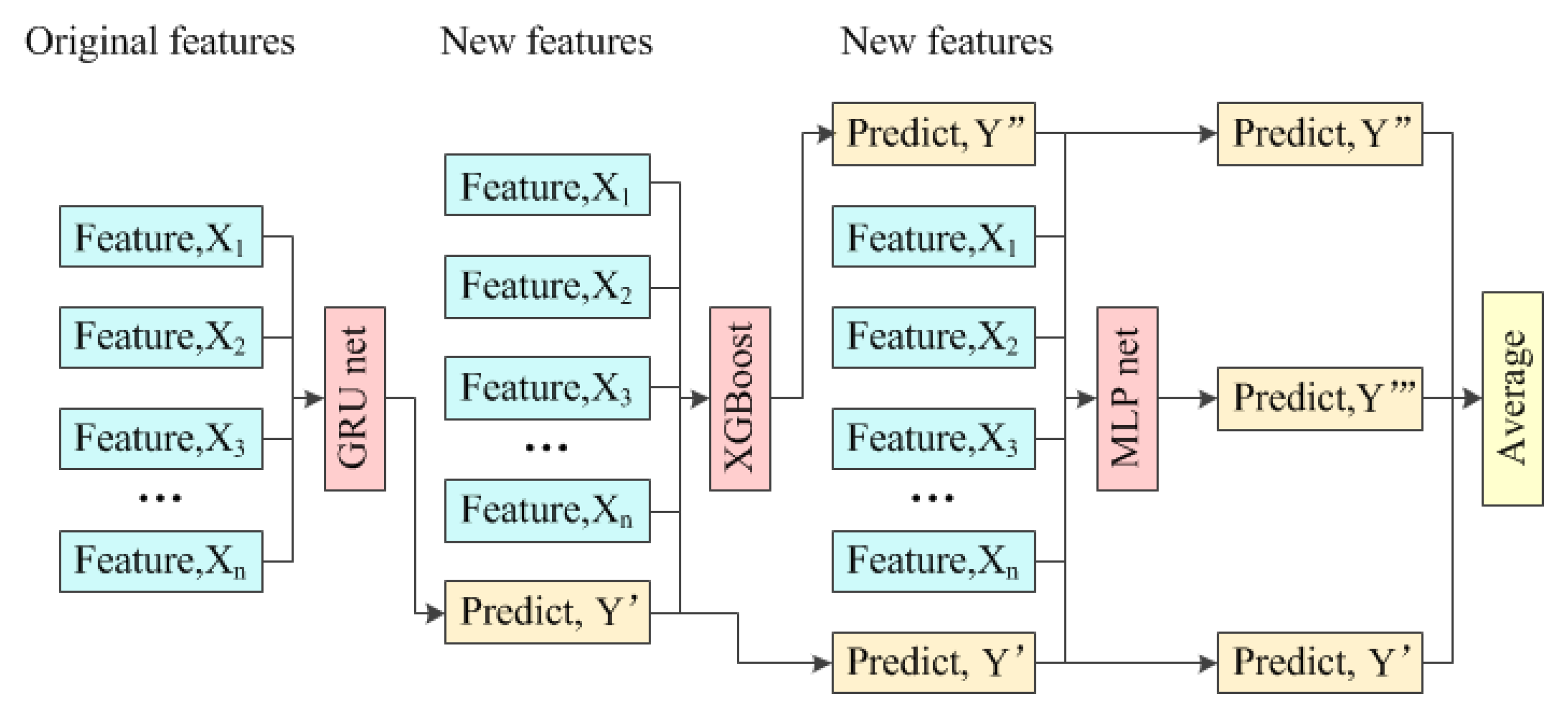
This paper tries to form an ensemble of three popular models to predict short-term photovoltaic power output; the principle is shown in Figure 1.
Firstly, a gated recurrent unit network (GRU) is trained with all original features, and the performance of the trained GRU network is tested based on a training set and a testing set. The original features and the predicted output power will form new features for the next model. Secondly, an XGBoost is trained with new features, and the performance of the trained XGBoost is also tested based on a training set and a testing set. The original features, the predicted output powers from the GRU network, and XGBoost again form new features for the next model. Thirdly, a multi-layer perceptron network (MLP) is trained with new features, and the performance of the trained MLP network is examined using the test set. Finally, the predicted output powers from the GRU network, XGBoost, and MLP network on the test set are averaged to get the final results.
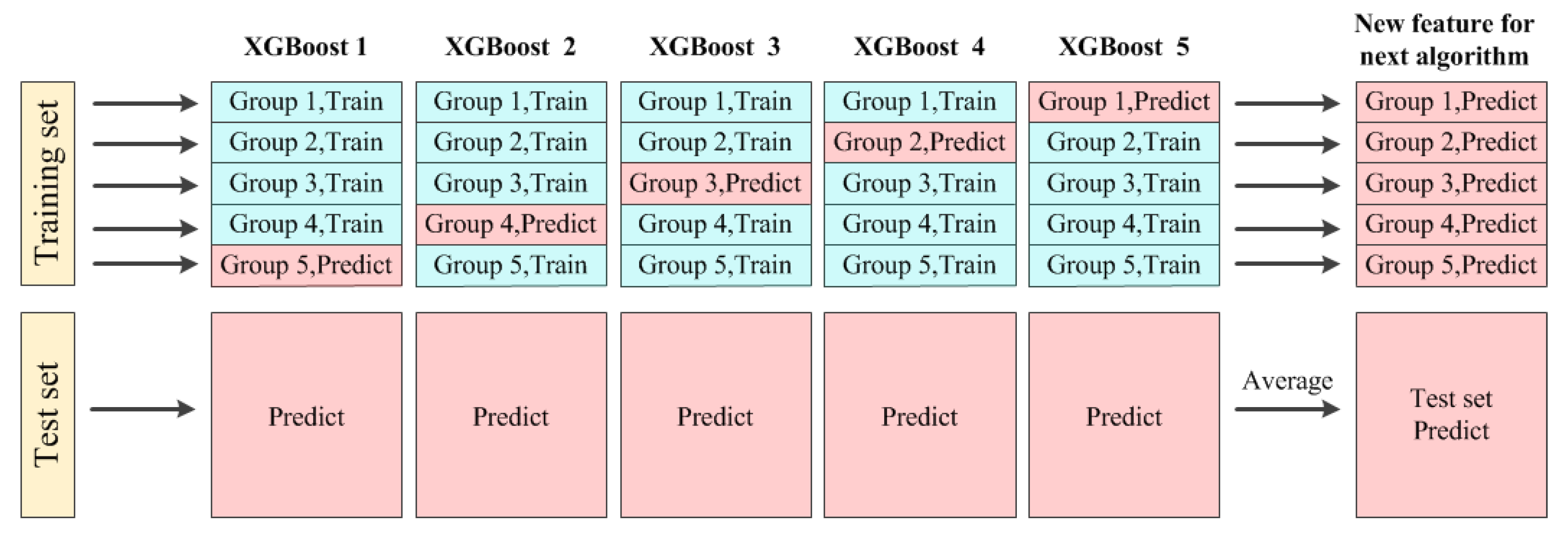
The ranking of the three models mentioned above is adjustable based on the testing results. The training methods of the GRU network, XGBoost, and MLP network are the same. XGBoost is taken as an example to illustrate the k-fold cross-validation method. The training process is shown in Figure 2.
Firstly, the training set is divided into k-many groups on average. The kth group of data is selected as a test sample and the remaining k − 1 groups of data are used to train the XGBoost. The trained XGBoost is used to predict the photovoltaic power output of the kth group and the photovoltaic power of the test set. Secondly, we select the data of the (k − 1)th group as the test sample, and the remaining k − 1 groups of data are used to train XGBoost. The trained XGBoost is used to predict the photovoltaic powers of the (k − 1)th group and the photovoltaic powers of the test set. Thirdly, repeating the above steps, there will be k-many XGBoost models and k-many groups of predicted data, which will constitute the predictive power of the training set. In addition, the predicted power of the training set will be used as a new feature to train the next model, such as an MLP network. Finally, the performance of the k trained XGBoost models is tested based on those k training sets. The average photovoltaic power of the test set is the result of the XGBoost model. It is noteworthy that k is 0 in the traditional training model.
3. Methodology
3.1. Data Cleaning
The data set used was from the short-term photovoltaic power forecasting competition held by China State Power Investment Corporation Limited in August 2018 (the data sets can be obtained from the following web site: https://github.com/Smilexuhc). The data set contains 9000 samples. The original features include photovoltaic panel operating state parameters and meteorological parameters, as shown in Table 1.
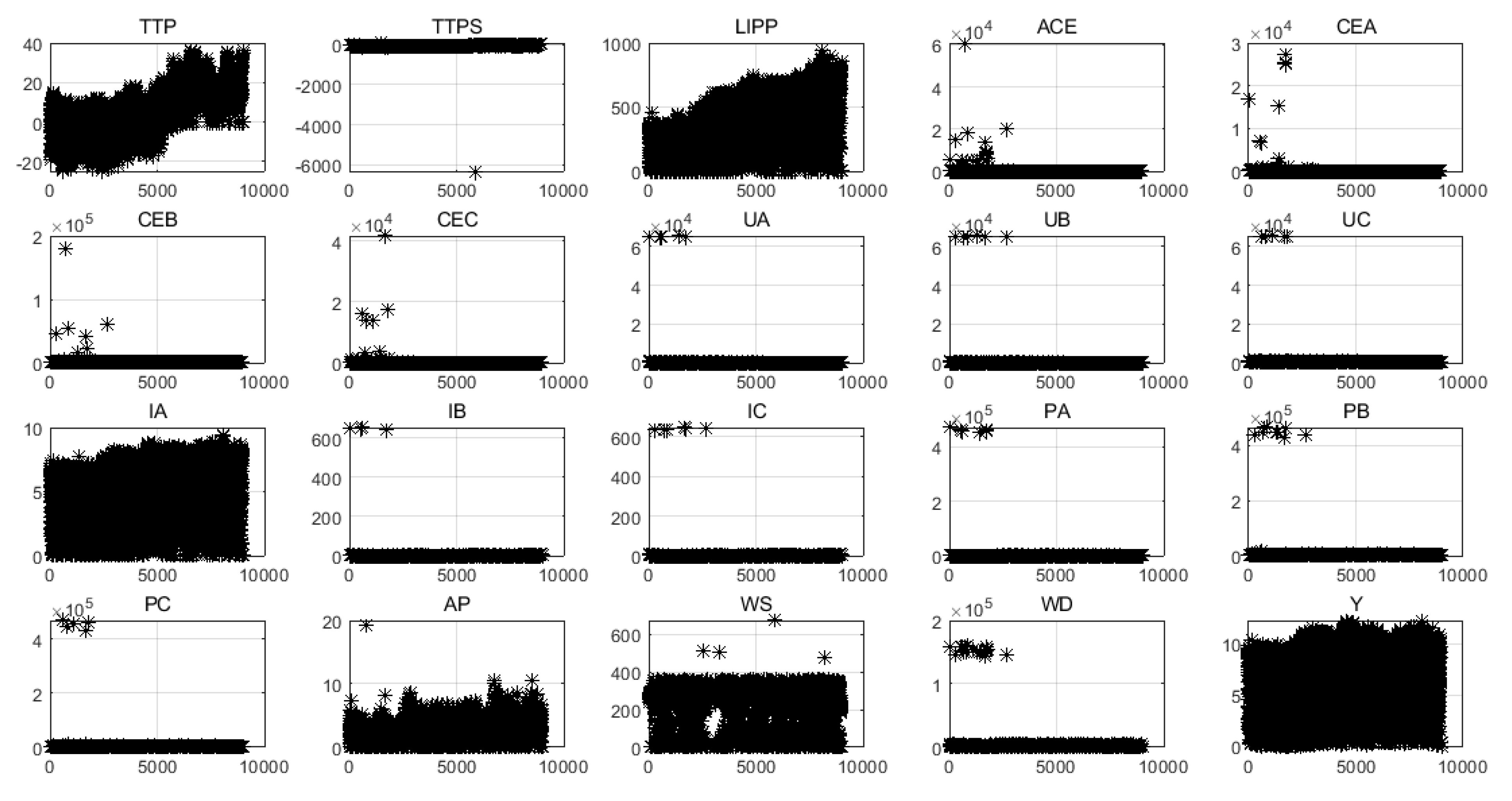
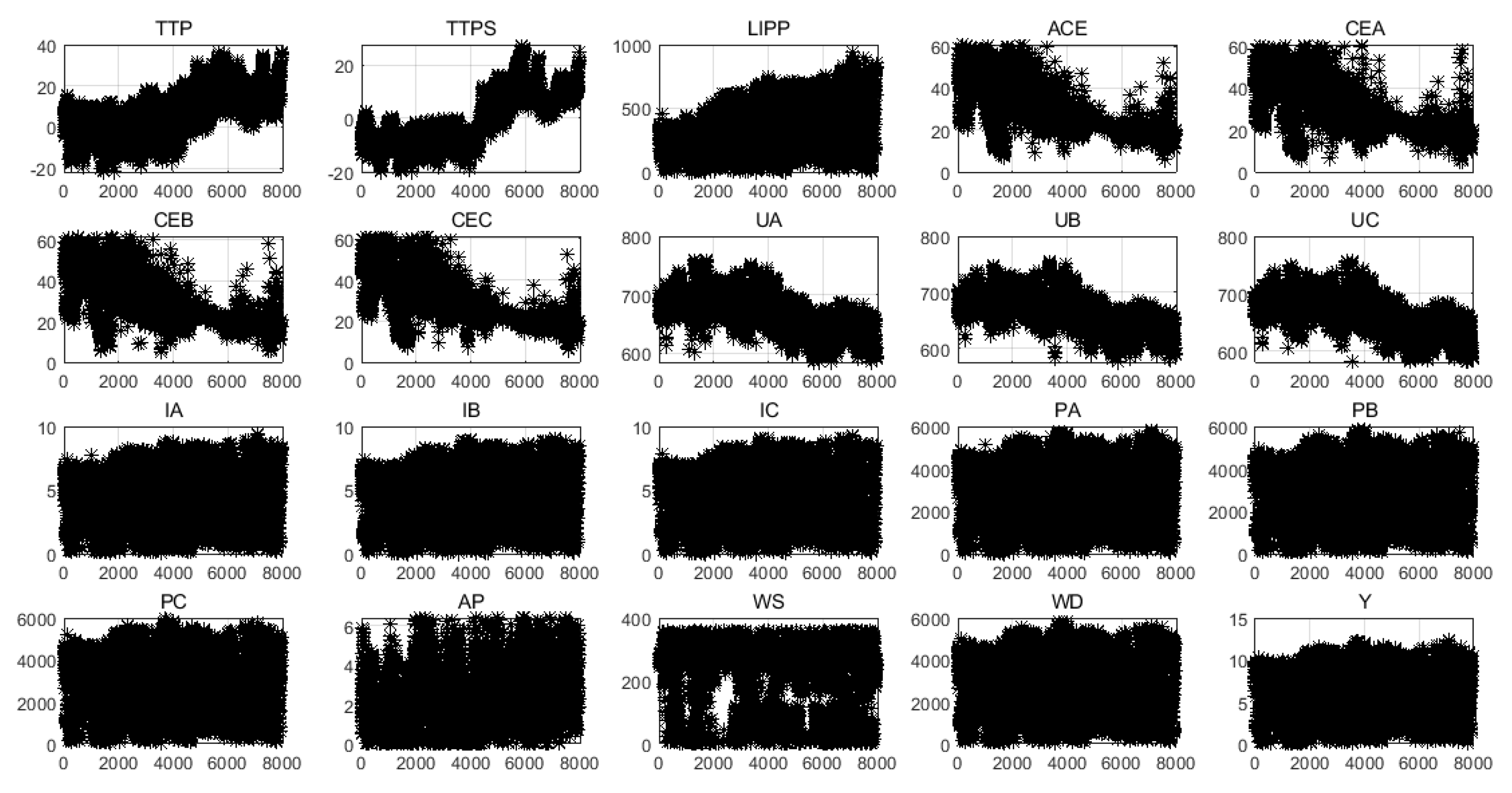
In order to analyze the characteristics of the data intuitively, 20 variables were visualized, as shown in Figure 3. Obviously, except for TTP, LIPP, IA, and Y, most variables have some outliers. The existence of outliers affects the training and prediction performance of the model. In order to eliminate the negative effects of those outliers, it is necessary to find the outliers of each variable and do some processing, such as replacing them with the average.
The quartile method is an important method used to analyze data distribution in statistics [19]. It is often used to identify outliers. The principle of the method is shown in Figure 4.
A set of data is arranged in ascending order, and they are divided into 4 parts. The three dividing points , , and are quartiles. The steps of using the quartile method to find outliers are as follows:
(1) The second quartile is calculated first, which is the median . The mathematical formula is as follows:
(2) We calculate the first quartile and third quartile in three different cases. In the first case, if n = 2k (k = 1, 2, …), X is divided into two groups with as the dividing point. The respective medians and of the two groups are calculated. Then the formulas for and are as follows:
In the second case, if n = 4k + 1(k = 1, 2, …), the formulas for and are as follows:
In the third case, if n = 4k + 3(k = 1, 2, …), the formulas for and are as follows:
(3) After calculating the quartiles, the interquartile range (IQR) is used to characterize the data when there may be extremities that skew the data. The formula for calculating the IQR is as follows:
(4) After determining the first and third quartiles and the interquartile range as outlined above, fences are calculated using the following formula:
The min is the "lower limit" and the max is the "upper limit" of data, and any data lying outside these defined bounds can be considered an outlier. Since the measured data is a time series, for outliers, we will directly use the last normal number instead of them.
3.2. Feature Selection
The output power of a photovoltaic power station is influenced by many factors, such as the performance of photovoltaic panels, meteorological conditions, operating conditions, and so on. The development of photovoltaic power generation is restricted due to its strong randomness. At present, most of the existing photovoltaic power prediction technologies only use meteorological conditions and historical data while ignoring the impact of photovoltaic panel performance and actual operating conditions, and the prediction accuracy of short-term power generation is limited. When establishing a short-term photovoltaic power prediction model, more factors affecting photovoltaic power should be considered to improve the prediction accuracy. If some insignificant factors are taken as input features, the accuracy may be reduced. Therefore, it is necessary to find a method to evaluate the correlation between various factors and photovoltaic power output.
In statistics, the Pearson correlation coefficient is widely used to measure the linear correlation between two variables X and Y [20,21]. It has a value between −1 and +1, where −1 is total negative linear correlation, 0 is no linear correlation, and +1 is total positive linear correlation. The formula for computing the Pearson correlation coefficient of two n-dimensional vectors X and Y is as follows:
where is the mean of X and is the mean of Y.
The Pearson coefficient method is used to evaluate the correlation between various factors and photovoltaic power. The statistical results are shown in Table 2.
From Table 2, the following conclusions were drawn: (1) The conversion efficiency and the voltage at each sampling point are negatively correlated with the photovoltaic power output, and other variables are positively correlated with the photovoltaic power output. (2) Since the correlations between conversion efficiencies and photovoltaic power output are weak, they were not selected as input features for the model.
3.3. Principle of the Prediction Algorithm
The MLP network, XGBoost, and GRU network were used as the three submodels of the ensemble model. This section mainly introduces the basic theory of the three algorithms.
3.3.1. XGBoost Model
The XGBoost algorithm was proposed by Dr. Chen Tianqi in 2014 [22]. It has attracted widespread attention in academia and industry due to its superior efficiency and high prediction accuracy. XGBoost is often used for supervised learning problems such as classification and regression. XGBoost’s weak learner is a decision tree. When training each decision tree, firstly, the weights of data with poor prediction accuracy are increased. Secondly, the current single decision tree is trained. Thirdly, by adding a new decision tree, the residual of all the previous decision trees can be corrected. Finally, the decision trees are added together to predict the short-term photovoltaic power output.
XGBoost algorithm is an additive model composed of several decision trees. Usually, the objective function consists of two parts: training loss and regularization [23]. The mathematical formula is as follows:
where K is the number of trees, is the output value of the kth tree, is a regularization that measures the complexity of the model and avoids overfitting, and represents the distance between and y, denoted , which is used to measure the training error. For short-term photovoltaic power forecasting, a common choice of l is the mean squared error. The mathematical formula is as follows:
In order to define the complexity of the tree, we need to refine the definition of the tree f(x) as
where q is a function assigning each data point to the corresponding leaf, w is the vector of scores on leaves, and T is the number of leaves. In XGBoost, we define the regularization as
where and are coefficients related to the regularization term. The XGBoost training and optimization are performed using the addition model and the forward stagewise algorithm. It assumes that is the predicted value of photovoltaic power at step t, and the iterative process is as follows:
where A is the decision tree to be trained in this step. Finally, the training objective function can be changed into
3.3.2. GRU Network
The GRU network is a special kind of recurrent neural network, proposed in 2014 by Kyunghyun Cho et al. [24]. It overcomes the problems of gradient disappearance and gradient explosion that plague traditional recurrent neural networks. It allows the creation of very large, very deep networks. Their performance in load forecasting and speech signal modeling was found to be similar to that of long short-term memory (LSTM). However, GRU has fewer parameters than LSTM, since it lacks an output gate. Unlike feedforward neural networks, GRU networks can use their internal memory to process a time series of inputs. This makes them applicable to time series prediction [25]. Therefore, a GRU network was selected as one of the submodels in this paper.
The GRU network unit structure is shown in Figure 5. The GRU unit is mainly composed of an update gate and a reset gate. The update gate is used to control whether the status information of the previous moment is brought into the current state. The larger the value of the update gate, the more status information of the previous moment is brought in. The reset gate is used to control whether the status information of the previous moment is lost. The smaller the value of the reset gate, the more information is lost. The relationship between the input and output of GRU units can be expressed as follows:
where is the input vector, is the output vector, is the update gate vector, is the reset gate vector, and W, U, and b are the parameter matrices and vector.
For GRU networks, popular training methods include backpropagation trough time (BPTT) and real-time recurrent learning (RTRL). Compared with RTRL, BPTT has higher computational efficiency and shorter computational time, so it was used to train the GRU network in this paper.
3.3.3. MLP Network
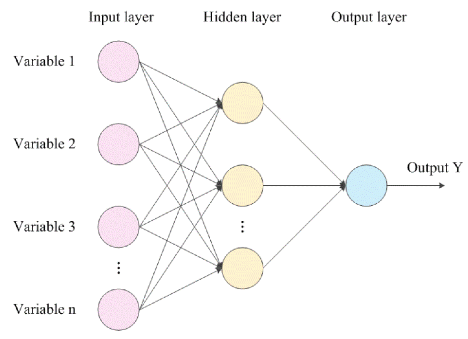
The MLP is a kind of forward-structured artificial neural network that maps a set of input vectors to a set of output vectors. It can be thought of as a directed graph, consisting of multiple node layers, each connected to the next layer. The structure of a classical MLP network is shown in Figure 6 and includes an input layer, hidden layer, and output layer. Except for the input nodes, each node is a neuron with a nonlinear activation function.
For the forward propagation process, the output of the hidden layer node can be expressed as
where n is the number of input layer nodes, q is the number of hidden layer nodes, is the weight between the ith node of the input layer and the kth node of the hidden layer, and is the activation function of the hidden layer.
Similarly, the relationship between the output layer and the hidden layer can be expressed as
where m is the number of output layer nodes, is the weight between the jth node of the output layer and the kth node of the hidden layer, and is the activation function of the output layer.
The MLP network maps n-dimensional input features to m-dimensional output variables based on Equation (17) and Equation (18). Generally, the network weights of the MLP are trained by the Back-Propagation method. The concrete deduction and mathematical formula of the backpropagation algorithm can be seen in the literature [26].
3.4. Statistical Metrics
In order to verify the effectiveness of the proposed methods, popular indicators such as the root-mean-square error (RMSE), mean absolute error (MAE), and mean absolute percentage error (MAPE) were used to evaluate the performance of different approaches. Their mathematical formulas are as follows:
where n is the number of samples in the test set, is the forecasted photovoltaic power, and is the real photovoltaic power.
3.5. The Process for Forecasting Photovoltaic Power Using the Ensemble Model
The steps for short-term photovoltaic power prediction using model ensemble techniques are as follows:
- (1)
- The quartile method is used to find outliers for each variable. These outliers are replaced by normal values from the previous moment.
- (2)
- The Pearson coefficient between each input factor and the photovoltaic power is calculated. The feature is selected as the input to the model based on the Pearson coefficient of each variable.
- (3)
- The selected features and photovoltaic power are normalized using a min–max normalization method to eliminate the negative effects of different units.
- (4)
- The training set is used to train MLP network, GRU network, and XGBoost. Then, the three models are used to predict the photovoltaic power of the test set.
- (5)
- The prediction results of the three models are combined according to the proposed ensemble framework, and the final predicted powers are output.
4. Case Study
4.1. The Test Settings
The data set used for testing includes 9000 samples. We randomly selected 80% of the samples as the training set and 10% of the data as the validation set. The remaining data was used as the test set. The proposed approaches were implemented using Tensorflow on a laptop equipped with an Intel(R) Core(TM) i7-6500M 3.20 GHz processor and 8 GB of RAM.
After many adjustments to the structure and parameters of the models, the optimum parameters of each model were set as follows: (1) For XGBoost, the maximum number of iterations was 15,000. The learning rate was 0.1. The RMSE was used as a valuation metric for the validation data. The maximum depth of a tree was 5. The learning objective was gamma regression with log-link. (2) For the LSTM network, the number of neurons in the input layer was equal to the number of input features. The hidden layer consisted of three LSTM layers with 10, 15, and 5 neurons, respectively. The activation function of the hidden layer was rectified linear unit function(ReLU). The output layer was a fully connected layer, and its number of neurons was 1. (3) For the MLP network, the number of neurons in the input layer was equal to the number of input features. The hidden layer consisted of three fully connected layers with 20, 10, and 5 neurons, respectively. The activation function of the hidden layer was ReLU. The output layer was a fully connected layer, and its number of neurons was 1.
The simulation was mainly composed of three parts: (1) The effect of outliers on prediction accuracy was analyzed. (2) The performances of the proposed training method and the traditional training method were tested. (3) The effect of the ordering of the three models on the prediction accuracy was explored.
4.2. Influence of Outliers on Prediction Accuracy
We visualized 20 variables through Figure 3 and found that there were some outliers in each variable. The outliers of each variable were selected using the quartile method and were replaced with the normal value of the previous timepoint. After data cleaning, the scatter plot of the 20 variables is shown in Figure 7.
Obviously, the values of each variable seem reasonable, and there are no so-called outliers. To illustrate the necessity of data cleaning, we calculated the prediction accuracy of the three models before and after data cleaning. Each model was run 30 times independently, and the statistical results are shown in Table 3.
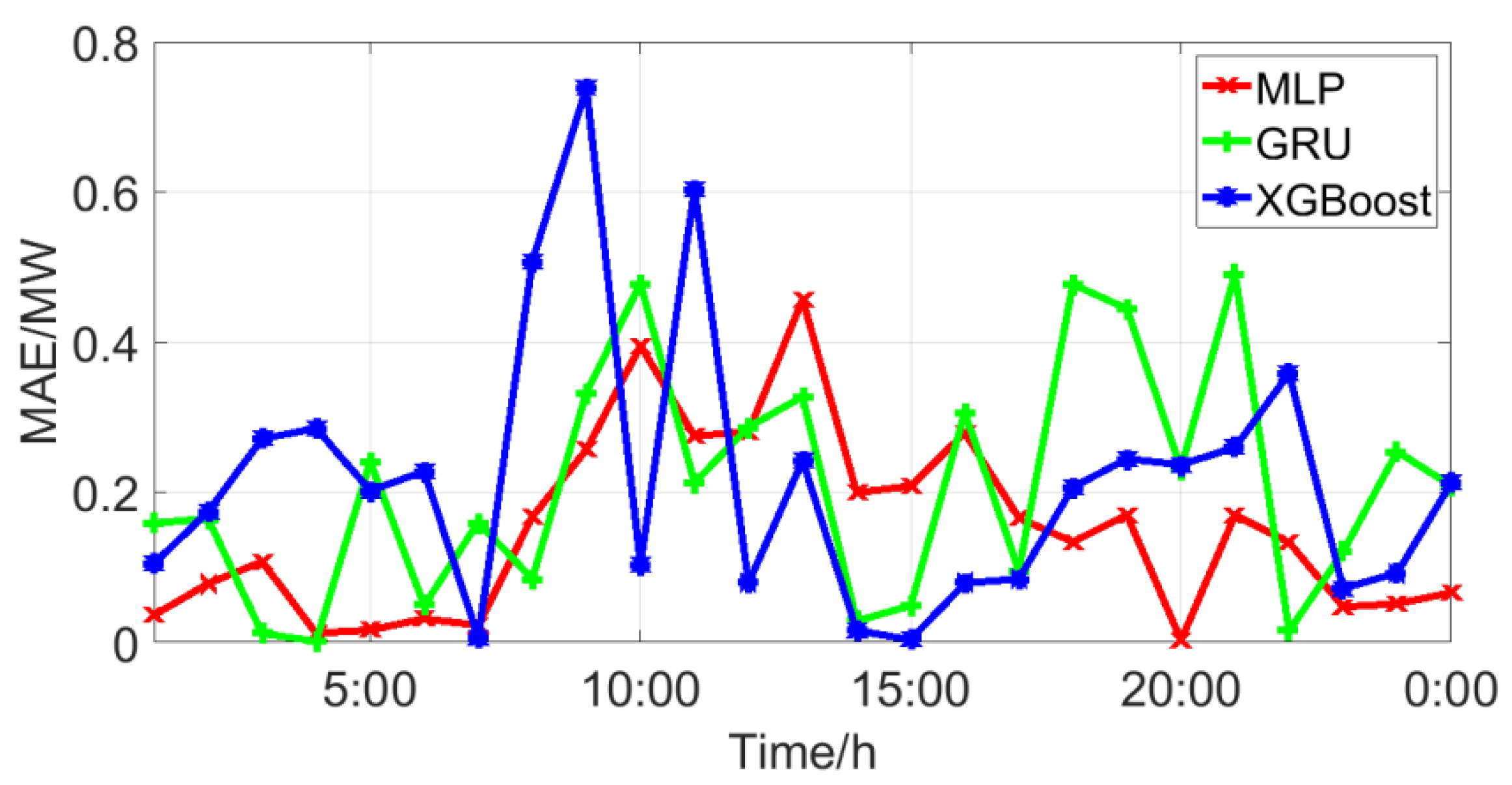
After data cleaning by the proposed method, the prediction accuracy of LSTM, MLP, and XGBoost was greatly improved, which shows the superiority of the proposed methods. As far as any single model is concerned, the prediction accuracy of MLP was higher than those of LSTM and XGBoost. Further, Figure 8 shows the MAPE of different models on a randomly selected day. Although MLP has the smallest average error, it has the greatest error at certain times, such as at 1:00 p.m.
4.3. The Performance of the Proposed Training Method
The MLP network is taken as an example to illustrate the effectiveness of k-fold cross-validation in the training model. We set k to vary from 0 to 45 with a step size of 5. Each case was repeated 40 times independently to obtain the mean of the predicted results. The statistical results are shown in Table 4.
From Table 4, we can draw the following conclusions: (1) As far as the error of the training set is concerned, the errors of the k-fold cross validation method (k > 0) are larger than that of the traditional training method (k = 0). With increasing k, the error of the training set decreases gradually. When k is equal to 0, all samples of the training set are used to train the model. When k is greater than 0, only some samples of the training set are used to train the model. Therefore, the k-fold cross-validation method has a larger prediction error than the traditional training method. (2) As far as the error of the test set is concerned, with increasing k, the error of test set decreases. When k is greater than 35, the training set error of the proposed method is larger than that of the traditional method, but the test set error of the proposed method is smaller than that of the traditional method. This phenomenon shows that the k-fold cross-validation method can improve the generalization ability of the model. (3) In terms of computing time, although k-fold cross-validation improves the accuracy of the test set, it increases the computing time of the model. The calculation time increases linearly with the increase of k. Therefore, the selection of k should take into account the calculation time and the accuracy of the test set.
4.4. Effect of Model Order on Accuracy
In order to analyze the influence of model order on prediction accuracy, we counted the errors of test sets for the six different model orders, and the statistical results are shown in Table 5.
Obviously, the position of each model in the ensemble model has a great impact on the prediction accuracy. Table 3 shows that MLP has the highest accuracy and GRU the worst. From Table 5, it can be seen that putting the model with highest accuracy ahead contributes to improving the prediction accuracy. In addition, the prediction accuracies of Case 1, Case 2, and Case 5 are lower than that of MLP, which shows that the prediction accuracy of model fusion cannot be guaranteed to be higher than that of a single model because the prediction accuracy is affected by the structure of the ensemble model and the positions of submodels. Case 3, Case 4, and Case 6 have higher prediction accuracy than MLP, which indicates that the ensemble model can achieve higher prediction accuracy than a single model by adjusting the structure.
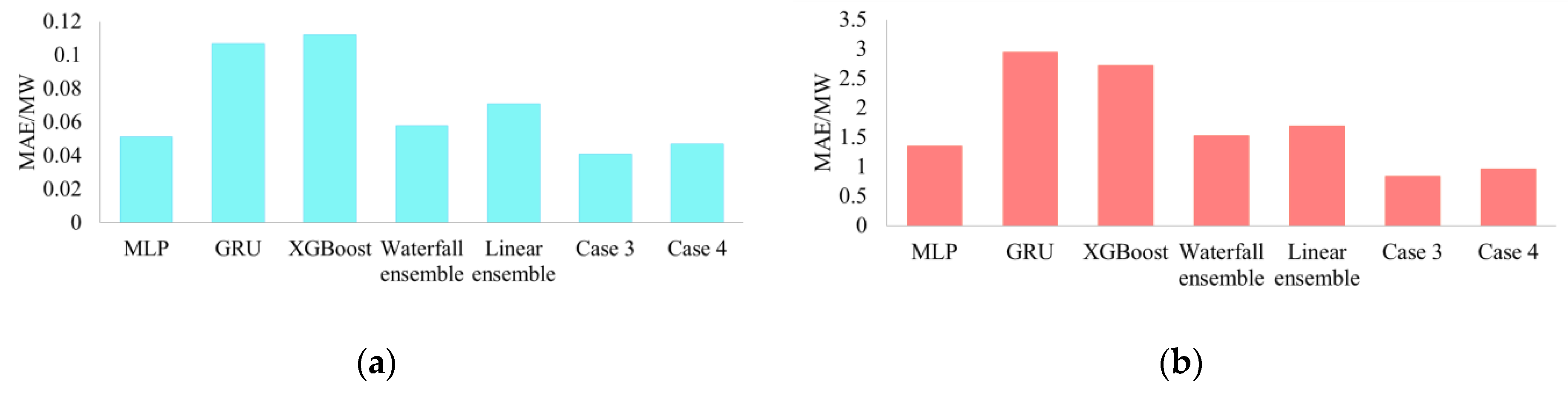
Furthermore, we calculated the error of the test set by different methods, and the statistical results are shown in Figure 9. The Waterfall ensemble refers to the sequential concatenation of MLP, GRU, and XGBoost [27]. The predicted results of MLP were used as the input for GRU. Similarly, the output of GRU served as the input to XGBoost. Finally, XGBoost output the predicted results. The Linear ensemble refers to training MLP, GRU, and XGBoost, respectively, and calculating the mean of the test set. The framework of the ensemble can be seen in reference [25]. Obviously, the Waterfall ensemble and Linear ensemble prediction errors are smaller than those of GRU and XGBoost but larger than that of MLP, which indicates that the traditional ensemble techniques need to be improved. Compared with the prediction errors of Case 3, Case 4, and other methods, we can conclude that the proposed method can not only reduce the average prediction error but also reduce the maximum prediction error.
5. Conclusions
It is of great practical significance for improving the operation of power systems and increasing the penetration of photovoltaic power to predict short-term photovoltaic power generation accurately. In this paper, we formed ensembles of multiple models in order to predict short-term photovoltaic power. The model ensemble technique can fully absorb the advantages of different algorithms and greatly improve the prediction accuracy. After simulations, we draw the following conclusions:
- (1)
- The quartile method can find outliers and help us clean the raw data, which is conducive to improving the prediction accuracy of the model.
- (2)
- The k-fold cross-validation method can improve the generalization ability of the models. With increasing k, the error of the test set decreases. However, the selection of k should take into account the calculation time and the accuracy of the test set.
- (3)
- The positions of the models have a great impact on the prediction accuracy when we form an ensemble of multiple models. Specifically, placing a single model with a small prediction error in front of the ensemble model can achieve better performance. The ensemble model can achieve higher prediction accuracy than a single model by adjusting the structure of the ensemble model.
- (4)
- The simulation results show that the average prediction error of the proposed method is smaller than those of single models and the traditional ensemble methods, and it can also reduce the maximum prediction error.
Author Contributions
Methodology, R.Z.; Software, W.G.; Writing—original draft, X.G.
Funding
This work was supported by the National High Technology Research and Development Program of China (Grant No. 2015AA050203) and the key project of Key Laboratory of Electrical Engineering Laboratory of Tibet Agriculture and Animal Husbandry University (Grant No. DQ2019ZD01).
Acknowledgments
The authors are grateful to China State Power Investment Corporation limited for the data set.
Conflicts of Interest
The authors declare no conflict of interest.
References
- Ariyaratna, P.; Muttaqi, K.M.; Sutanto, D. A novel control strategy to mitigate slow and fast fluctuations of the voltage profile at common coupling point of rooftop solar PV unit with an integrated hybrid energy storage system. J. Energy Storage 2018, 20, 409–417. [Google Scholar] [CrossRef]
- Wang, Z.; Gu, C.; Li, F. Flexible operation of shared energy storage at households to facilitate PV penetration. Renew. Energy 2018, 116, 438–446. [Google Scholar] [CrossRef]
- Sepasi, S.; Reihani, E.; Howlader, A.M.; Roose, L.R.; Matsuura, M.M. Very short term load forecasting of a distribution system with high PV penetration. Renew. Energy 2017, 106, 142–148. [Google Scholar] [CrossRef]
- Yang, D.; Kleissl, J.; Gueymard, C.A.; Pedro, H.T.C.; Coimbra, C.F.M. History and trends in solar irradiance and PV power forecasting: A preliminary assessment and review using text mining. Sol. Energy 2018, 168, 60–101. [Google Scholar] [CrossRef]
- Eseye, A.T.; Zhang, J.; Zheng, D. Short-term photovoltaic solar power forecasting using a hybrid wavelet-pso-svm model based on scada and meteorological information. Renew. Energy 2018, 118, 357–367. [Google Scholar] [CrossRef]
- Raza, M.Q.; Nadarajah, M.; Ekanayake, C. Demand forecast of pv integrated bioclimatic buildings using ensemble framework. Appl. Energy 2017, 208, 1626–1638. [Google Scholar] [CrossRef]
- El-Baz, W.; Tzscheutschler, P.; Wagner, U. Day-ahead probabilistic PV generation forecast for buildings energy management systems. Sol. Energy 2018, 171, 478–490. [Google Scholar] [CrossRef]
- Wang, F.; Zhang, Z.; Liu, C.; Yu, Y.; Pang, S.; Duić, N.; Shafie-khah, M.; Catalão, J.P.S. Generative adversarial networks and convolutional neural networks based weather classification model for day ahead short-term photovoltaic power forecasting. Energy Convers. Manag. 2019, 181, 443–462. [Google Scholar] [CrossRef]
- Raza, M.Q.; Nadarajah, M.; Ekanayake, C. On recent advances in pv output power forecast. Sol. Energy 2016, 136, 125–144. [Google Scholar] [CrossRef]
- Ma, T.; Yang, H.; Lu, L. Solar photovoltaic system modeling and performance prediction. Renew. Sustain. Energy Rev. 2014, 36, 304–315. [Google Scholar] [CrossRef]
- Lorenz, E.; Hurka, J.; Heinemann, D.; Beyer, H.G. Irradiance forecasting for the power prediction of grid-connected photovoltaic systems. IEEE J. Sel. Top. Appl. Earth Obs. Remote Sens. 2009, 2, 2–10. [Google Scholar] [CrossRef]
- Hossain, M.; Mekhilef, S.; Danesh, M.; Olatomiwa, L.; Shamshirband, S. Application of extreme learning machine for short term output power forecasting of three grid-connected PV systems. J. Clean. Prod. 2017, 167, 395–405. [Google Scholar] [CrossRef]
- Li, P.; Zhang, J.-S. A new hybrid method for China’s energy supply security forecasting based on arima and xgboost. Energies 2018, 11, 1687. [Google Scholar] [CrossRef]
- Zhang, W.; Quan, H.; Srinivasan, D. Parallel and reliable probabilistic load forecasting via quantile regression forest and quantile determination. Energy 2018, 160, 810–819. [Google Scholar] [CrossRef]
- Abdel-Nasser, M.; Mahmoud, K. Accurate photovoltaic power forecasting models using deep LSTM-RNN. Neural Comput. Appl. 2017. [Google Scholar] [CrossRef]
- Xiao, Y.; Wu, J.; Lin, Z.; Zhao, X. A deep learning-based multi-model ensemble method for cancer prediction. Comput. Methods Programs Biomed. 2018, 153, 1–9. [Google Scholar] [CrossRef]
- Yun, K.; Hsiao, J.; Jung, M.-P.; Choi, I.-T.; Glenn, D.M.; Shim, K.-M.; Kim, S.-H. Can a multi-model ensemble improve phenology predictions for climate change studies? Ecol. Model. 2017, 362, 54–64. [Google Scholar] [CrossRef]
- Xiao, J.; Li, Y.; Xie, L.; Liu, D.; Huang, J. A hybrid model based on selective ensemble for energy consumption forecasting in China. Energy 2018, 159, 534–546. [Google Scholar] [CrossRef]
- Carling, K. Resistant outlier rules and the non-gaussian case. Comput. Stat. Data Anal. 2000, 33, 249–258. [Google Scholar] [CrossRef]
- Zhou, H.; Deng, Z.; Xia, Y.; Fu, M. A new sampling method in particle filter based on pearson correlation coefficient. Neurocomputing 2016, 216, 208–215. [Google Scholar] [CrossRef]
- Kim, N.; Park, S.; Lee, J.; Choi, K.J. Load profile extraction by mean-shift clustering with sample pearson correlation coefficient distance. Energies 2018, 11, 2397. [Google Scholar] [CrossRef]
- Chen, T.; Guestrin, C. In Xgboost: A scalable tree boosting system. In Proceedings of the ACM Sigkdd International Conference on Knowledge Discovery & Data Mining, San Francisco, CA, USA, 13–17 August 2016. [Google Scholar]
- Zheng, H.; Yuan, J.; Chen, L. Short-term load forecasting using emd-lstm neural networks with a xgboost algorithm for feature importance evaluation. Energies 2017, 10, 1168. [Google Scholar] [CrossRef]
- Cho, K.; Van Merrienboer, B.; Gulcehre, C.; Bahdanau, D.; Bougares, F.; Schwenk, H.; Bengio, Y. Learning phrase representations using RNN encoder-decoder for statistical machine translation. arXiv, 2014; arXiv:1406.1078. [Google Scholar]
- Wang, Y.; Liao, W.; Chang, Y. Gated recurrent unit network-based short-term photovoltaic forecasting. Energies 2018, 11, 2163. [Google Scholar] [CrossRef]
- Horikawa, S.; Furuhashi, T.; Uchikawa, Y. On fuzzy modeling using fuzzy neural networks with the back-propagation algorithm. IEEE Trans. Neural Netw. 1992, 3, 801–806. [Google Scholar] [CrossRef] [PubMed]
- Sun, Z. A waterfall model for knowledge management and experience management. In Proceedings of the Fourth International Conference on Hybrid Intelligent Systems (HIS’04), Kitakyushu, Japan, 5–8 December 2004; pp. 472–475. [Google Scholar]
Figure 1.
The principle of the model ensemble.

Figure 2.
The principle of the k-fold cross-validation method.

Figure 3.
Visual analysis of 20 variables.

Figure 4.
The principle of quartiles.

Figure 5.
The architecture of the gated recurrent unit.

Figure 6.
An example of an MLP network with one hidden layer.

Figure 7.
Visual analysis of 20 variables after data cleaning.

Figure 8.
MAE values of the different models.

Figure 9.
Statistical results of each method: (a) average MAE of each method and (b) maximum MAE of each method.
Figure 9.
Statistical results of each method: (a) average MAE of each method and (b) maximum MAE of each method.


Table 1.
Variables and description.
| Variable Name | Mark | Variable Name | Mark |
|---|---|---|---|
| Temperature of photovoltaic panel | TPP | Light intensity in photovoltaic plant | LIPP |
| Temperature of photovoltaic power station | TPPS | Wind speed in photovoltaic plant | WS |
| Conversion efficiency of photovoltaic panel at sampling point A | CEA | Conversion efficiency of photovoltaic panel at sampling point B | CEB |
| Conversion efficiency of photovoltaic panel at sampling point C | CEC | Average conversion efficiency of A,B,C | ACE |
| Voltage of convergence box at sampling point A | UA | Voltage of convergence box at sampling point B | UB |
| Voltage of convergence box at sampling point C | UC | Current of convergence box at sampling point A | IA |
| Current of convergence box at sampling point B | IB | Current of convergence box at sampling point C | IC |
| Power at sampling point A | PA | Power at sampling point B | PB |
| Power at sampling point C | PC | Average power of A,B,C | AP |
| Wind direction of photovoltaic plant | WD | Photovoltaic power to be predicted | Y |
Table 2.
The Pearson coefficients between variables and photovoltaic power.
| Variables | Pearson | Variables | Pearson | Variables | Pearson | Variables | Pearson |
|---|---|---|---|---|---|---|---|
| TTP | 0.505 | CEB | −0.033 | IA | 0.994 | PC | 0.989 |
| TTPS | 0.151 | CEC | −0.063 | IB | 0.978 | AP | 0.997 |
| LIPP | 0.875 | UA | −0.299 | IC | 0.988 | WS | 0.102 |
| ACE | −0.048 | UB | −0.311 | PA | 0.997 | WD | 0.185 |
| CEA | −0.040 | UC | −0.310 | PB | 0.978 |
Table 3.
The statistical results under different circumstances.
| Model | Data Cleaning | No Data Cleaning | ||||
|---|---|---|---|---|---|---|
| RMSE | MAE | MAPE | RMSE | MAE | MAPE | |
| MLP | 0.125 | 0.051 | 2.48% | 0.233 | 0.112 | 5.36% |
| GRU | 0.168 | 0.107 | 5.12% | 0.222 | 0.121 | 6.84% |
| XGBoost | 0.183 | 0.112 | 4.91% | 0.208 | 0.118 | 5.77% |
Table 4.
The statistical results under different circumstances.
| Training Set | Test Set | k | Time for Each Calculation/s | ||||
|---|---|---|---|---|---|---|---|
| RMSE | MAE | MAPE | RMSE | MAE | MAPE | ||
| 0.137 | 0.034 | 1.38% | 0.128 | 0.051 | 2.25% | 0 | 2.27 |
| 0.150 | 0.050 | 2.11% | 0.129 | 0.053 | 2.41% | 5 | 11.06 |
| 0.146 | 0.043 | 1.81% | 0.128 | 0.051 | 2.30% | 10 | 22.90 |
| 0.146 | 0.042 | 1.73% | 0.127 | 0.050 | 2.27% | 15 | 34.93 |
| 0.146 | 0.041 | 1.73% | 0.128 | 0.051 | 2.25% | 20 | 45.60 |
| 0.144 | 0.040 | 1.68% | 0.128 | 0.050 | 2.25% | 25 | 57.26 |
| 0.143 | 0.040 | 1.64% | 0.128 | 0.050 | 2.24% | 30 | 67.49 |
| 0.143 | 0.039 | 1.65% | 0.128 | 0.050 | 2.23% | 35 | 77.90 |
| 0.143 | 0.039 | 1.63% | 0.127 | 0.050 | 2.21% | 40 | 102.05 |
| 0.142 | 0.038 | 1.61% | 0.127 | 0.049 | 2.21% | 45 | 112.44 |
Table 5.
Impact of model order on results.
| Scheme | Order of Models | RMSE | MAE | MAPE |
|---|---|---|---|---|
| Case 1 | GRU,XGBoost,MLP | 0.147 | 0.068 | 3.25% |
| Case 2 | XGBoost,GRU,MLP | 0.143 | 0.076 | 2.85% |
| Case 3 | MLP,GRU,XGBoost | 0.094 | 0.041 | 1.60% |
| Case 4 | MLP,XGBoost,GRU | 0.117 | 0.047 | 1.85% |
| Case 5 | GRU,MLP,XGBoost | 0.130 | 0.064 | 3.38% |
| Case 6 | XGBoost,MLP,GRU | 0.121 | 0.061 | 2.13% |
© 2019 by the authors. Licensee MDPI, Basel, Switzerland. This article is an open access article distributed under the terms and conditions of the Creative Commons Attribution (CC BY) license (http://creativecommons.org/licenses/by/4.0/).
Share and Cite
MDPI and ACS Style
Zhu, R.; Guo, W.; Gong, X. Short-Term Photovoltaic Power Output Prediction Based on k-Fold Cross-Validation and an Ensemble Model. Energies 2019, 12, 1220. https://0-doi-org.brum.beds.ac.uk/10.3390/en12071220
AMA Style
Zhu R, Guo W, Gong X. Short-Term Photovoltaic Power Output Prediction Based on k-Fold Cross-Validation and an Ensemble Model. Energies. 2019; 12(7):1220. https://0-doi-org.brum.beds.ac.uk/10.3390/en12071220
Chicago/Turabian StyleZhu, Ruijin, Weilin Guo, and Xuejiao Gong. 2019. "Short-Term Photovoltaic Power Output Prediction Based on k-Fold Cross-Validation and an Ensemble Model" Energies 12, no. 7: 1220. https://0-doi-org.brum.beds.ac.uk/10.3390/en12071220
Note that from the first issue of 2016, this journal uses article numbers instead of page numbers. See further details here.