An Experimental Investigation of a Novel Low-Cost Photovoltaic Panel Active Cooling System


Department of Industrial Engineering, University of Padova, 35100 Padova, Italy
*
Author to whom correspondence should be addressed.
Energies 2019, 12(8), 1448; https://0-doi-org.brum.beds.ac.uk/10.3390/en12081448
Submission received: 10 March 2019
/
Revised: 8 April 2019
/
Accepted: 10 April 2019
/
Published: 16 April 2019
(This article belongs to the Section A2: Solar Energy and Photovoltaic Systems)
Abstract
:Renewable energy sources are the most useful way to generate clean energy and guide the transition toward green power generation and a low-carbon economy. Among renewables, the best alternative to electricity generation from fossil fuels is solar energy because it is the most abundant and does not release pollutants during conversion processes. Despite the photovoltaic (PV) module ability to produce electricity in an eco-friendly way, PV cells are extremely sensitive to temperature increments. This can result in efficiency drop of 0.25%/C to 0.5%/C. To overcome this issue, manufacturers and researchers are devoted to the improvement of PV cell efficiency by decreasing operating temperature. For this purpose, the authors have developed a low-cost and high-performance PV cooling system that can drastically reduce module operating temperature. In the present work, the authors present a set of experimental measurements devoted to selecting the PV cooling arrangement that guarantees the best compromise of water-film uniformity, module temperature reduction, water-consumption minimization, and module power production maximization. Results show that a cooling system equipped with 3 nozzles characterized by a spraying angle of 90, working with an inlet pressure of 1.5 bar, and which remains active for 30 s and is switched off for 120 s, can reduce module temperature by 28 C and improve the module efficiency by about 14%. In addition, cost per single module of the cooling system is only 15 €.
1. Introduction
Energy is the driving force of our society and its availability at reasonable prices influences countries’ development and standard of living.
At worldwide level, about one billion people out of 7.5 billion have no access to electricity. However, these people live in geographical areas, mainly sub-Saharan Africa, rich in both fossil fuels and renewable resources and characterized by the highest 2017 regional real gross domestic product (GDP) growth rate: +3.8% [1]. Despite these key factors, no access to electricity implies an extremely low standard of living, as well as living below the poverty threshold. In fact, the sub-Saharan African population is among the poorest in the world.
Therefore, the energy sector and, in particular, electricity, is essential not only for the social and economic development of the world population, but also for their quality of life. Urbanization and industrialization, as well as a high standard of living, are strictly linked to energy availability. In particular, they rely on the ability to meet an ever-growing energy demand by means of cheap energy sources, a fact still guaranteed by fossil fuels.
Ten years of primary energy consumption analysis [2] shows a world that continues to grow at a yearly average rate of 1.6%. In 2007, 11,588.4 Mtoe were consumed, while in 2017, the primary energy consumption was 13,511.2 Mtoe. The Organization for Economic Co-operation and Development (OECD) countries’ primary energy consumption has remained approximately constant over the last decade (5693.9 Mtoe vs. 5605.0 Mtoe) while non-OECD ones have risen from 5897.5 Mtoe to 7906.1 Mtoe. Thus, in the past decade, the primary energy consumption has moved geographically from OECD countries to developing ones (China chief among them).
Among the 13,511.2 Mtoe consumed around the world, about 85% came from fossil fuels. Thus, the world’s primary energy consumption is still covered by non-renewable sources.
Clearly, this is a slightly lower value compared to 2005, when it stood at 92%, but is still very high because, in 2017, oil, coal, and natural gas contributed for 34.2%, 27.6%, and 23.4%, respectively, of the world’s primary energy consumption [2].
Regarding other sources, nuclear energy stood at 4.4%, while renewable energy sources (RES) reached 10.4%: 6.8% from hydro-electricity and 3.6% from other renewables, where wind and solar represented only 0.6% and 1.9%, respectively [2].
In 2017, despite
- Skyrocketing annual development in terms of installed capacity of wind (+21%) and solar (+47%).
- The 279.8 billion US Dollars (bil US$) of global investment in renewable power and biofuels.
- The 70% of net additions to global power capacity coming from RES plants.
The latest estimations of global energy-related carbon dioxide (CO) emissions have increased by 1.4%.
Environmental effects of anthropic CO emissions are presently of great concern at a worldwide level but the European Union (EU), due to their fossil fuel shortage and the population’s increasing awareness over global warming and fossil-based power units environmental issues, is the only region where primary energy consumption and CO emissions have registered a progressive reduction, from 1823.9 Mtoe to 1689.2 Mtoe (period 2007–2017) and −9.4% (period 2005–2016), respectively.
The EU primary energy consumption drop is the result of a series of environmental protection actions devoted to greenhouse gas (GHG) emission reduction, the spread of RES, and energy efficiency rise.
The process started in the early 1990s when the EU stated that spreading RES, improving energy efficiency and mitigating power system carbon footprints are actions that can help to improve energy security and abate environmental pollution. For this purpose, the EU developed directives and a roadmap which progressively fixed targets in terms of GHG emissions reduction, RES spread, and energy efficiency rise for 2020, 2030, and 2050 [5,6,7].
At the time of writing, the EU member states are working to meet the targets fixed in the Directive 2009/28/EC [5].
In Reference [5], the EU set, for 2020, a 20% reduction of GHG emissions based on 1990 levels, with 20% of energy coming from renewable energy and a rise of 20% of energy efficiency. Yearly targets are set at EU level as well as at country level for each renewable resources, while each member state, by means of its own national renewable energy action plan (NREAP), established commitments and initiatives that the country intends to put into force to develop the RES sector and fulfil the 2020 prescribed targets. In particular, each country set an overall target and targets for heating and cooling, electricity, and transport as well as the support policies.
As an example, the Italian NREAP report [8] established an overall target that in gross final energy consumption prescribes a 17% share of energy generated from renewable sources. In the electricity sector, a target of 26% of electricity demand met by electricity generated from RES is set, while in transport, the target is 10% of energy demand being met by renewables. Regarding heating and cooling, 17% of heat consumption will be met by renewable sources.
Obviously, to fulfil the above-mentioned targets’ feed-in tariffs, energy efficiency credits, renewable building hot water obligations, green certificates, quota system for electricity generated from renewable, biofuel transport quotas, tax relief for biofuels, and financial support for research and development activities [9] were put into force.
Support schemes are essential instruments that need to be put in place by governments to assist RES development and environmental protection actions, but incentive policies need also to be reviewed periodically to avoid market distortion.
Since the actions agreed upon in [5] are limited to 2020, the EU ratified the 2030 framework for climate and energy and the 2050 low-carbon economy roadmap [6,7] with the aim of continuing to foster RES after 2020.
In Reference [6], the reduction of GHG emissions for 2030 is set to 40% of 1990 levels, while targets for energy-saving and energy consumption produced from RES are set both at 27%.
The 2050 low-carbon economy roadmap [7] sets an ambitious target: a cut of 80% of GHG emissions from 1990 levels; a target achievable only if, in 2030 and 2040, the GHG emission cuts reach a 40% and 60% reduction from 1990 levels, respectively.
As mentioned above, to boost RES spread, governments have established generous financial supports (see, e.g., for the Italian PV sector Section 2) which has resulted in strong growth of on- and off-shore wind power and solar PV electricity generation.
For example, in 2017, 85% of all newly installed power capacity in the EU was of renewable origin; wind power and solar PV accounted for three quarters of the annual RES power capacity increment.
However, despite PV modules and wind turbines being able to generate electricity in an eco-friendly way, source variability and unpredictability can cause large unforeseeable fluctuations in power production at daily, weekly, monthly, or even annual level.
However, since it is essential to balance the electricity demand instantaneously 24/7, any mismatch between supply and demand can be the source of local instability, which in turn can cause local or even global grid damage, user device fault, or local and global blackouts.
Therefore, as stated in several research works (see, e.g., [10,11,12,13,14,15,16]), to prevent such damaging situations, fossil fuel power stations need to be used as back-up units, and electricity energy storage systems need to be installed.
Leaving aside the variable and intermittent nature of solar energy that causes PV production fluctuations, PV cell electricity generation is moreover affected by another parameter: the cell operating temperature.
PV cells absorb 80% of incident solar radiation, but they do not entirely convert it into electricity because PV cell manufacturing technology strongly affects the conversion efficiency. As reported in [17], PV modules reach a conversion efficiency in the range of 15–20%. However, as stated in [18], in the past 10 years, the average efficiency of commercial wafer-based silicon modules has risen from about 12% to 17% while, the cadmium telluride (CdTe) photovoltaic module efficiency has increased from 9% to 16%.
The record lab cell efficiency is 26.7% for monocrystalline and 22.3% for multicrystalline silicon wafer-based technology, while the highest lab efficiency in thin film technology is 22.9% for copper indium gallium (di)selenide (CIGS) and 21.0% for CdTe solar cells [18].
Again, in laboratory-scale applications, the best performing modules are based on monocrystalline silicon with 24.4% efficiency, while high-concentration multijunction solar cells achieve an efficiency of up to 46.0%. With concentrator technology, module efficiency of up to 38.9% can be reached [18].
These records in module and cell efficiency demonstrate the potential for further efficiency increases at the production level, even if the most efficient solar panel available on the market reaches only an efficiency of 22.2% [19].
Therefore, most of the solar irradiance is converted into heat, which results in an increment of the cell operating temperature and a reduction of the module efficiency (8–9%) [17].
Temperature increments have an extreme influence on solar cell operating parameters [20,21,22,23,24]: the open-circuit voltage is reduced by 2.0–2.3 mV/C, the fill factor diminishes by 0.1–0.2%/C, the power output cut is in the range 0.4–0.5%/C while only the circuit current rises, by 0.06–0.1%/C.
Also, irreversible damage to cell materials can occur. However, the most important consequence of temperature rise is efficiency reduction: experimental investigations observed efficiency reduction from 0.25%/C to 0.5%/C.
Therefore, to limit efficiency degradation of in-operation PV cells, there is only one feasible option: installing a cooling system. Obviously, a cooling system needs to be adaptable and easy to mount (especially to in-operation PV facilities), with high efficiency, and available with low purchase and operation costs.
In recent years, a large variety of studies have proposed methods to cool PV modules for the sole purpose of improving power output. Radiative cooling has been investigated by Safi and Munday [25] while, e.g., Moharram et al. [26], Nižetić et al. [27], and Zsiborács et al. [28] have studied water-sprayed cooling techniques. Evaporative cooling, forced air flow, and natural vaporization have been investigated by, e.g., Alami [29], Rahimi et al. [30], and Ebrahimi et al. [31] while cooling methods employing heat pipes or sprinkling techniques have been examined by Zhang et al. [32] and Bai et al. [33], respectively.
Generally speaking, PV cooling systems can be grouped as (i) consolidated technologies, and (ii) in-development techniques. Passive and active cooling methods are the consolidated and commercially available technologies, while liquid immersion cooling, cooling using Phase Change Material (PCM), colorless and lucid silicon coating, microporous evaporation foils, and thermoelectric cooling systems based on the Peltier effects, are in-development technologies [34,35,36].
Passive cooling systems act without an external source of power, while active ones require fans or pumps to operate the cooling medium, which is typically air or water. Active cooling systems are characterized by higher performance than passive ones [17,37]. In fact, experimental analyses show a temperature reduction up to 30 C for active cooling methods against a reduction of up to 20 C in cases of passive cooling systems. Active methods generally guarantee an electric efficiency improvement of up to 22%, compared to 15% in the case of passive methods [38,39].
The simplest passive cooling system consists of natural air circulation over and under the PV module, but in recent studies the insertion of material such as cotton wick in combination with water, /water nanofluid and /water nanofluid has been explored as a passive cooling system for flat PVs [40]. A summary of the current research related to the passive cooling system is available in [41].
A water film that flows on the module front or back or on both sides is the most studied and applied active cooling technique but in recent years innovative approaches that use converging channel heat exchangers or micro-channels have been developed and tested [42,43]. Regarding passive cooling techniques, recent advancements in an active cooling system can be found in [39].
Adopting an active cooling system guarantees performance improvements, but it is necessary to estimate its power consumption and, in the case of water active cooling methods, water consumption. Only if the extra electricity production is higher than the energy consumed by the cooling system itself is the proposed method feasible.
As mentioned above, other cooling techniques include liquid immersion and cooling by means of PCM. In the first case, PV cells are covered with a thin layer of a dielectric liquid such as glycerin, isopropyl alcohol, acetone, butanol, or water. In the second case, PCMs cool the PV module by absorbing its heat, but the absorbed heat changes the PCM’s phase (e.g., from solid to liquid). Then, water is used to cool the PCM, which ejects heat into the environment. This last method of cooling PV modules is an important research topic (see, e.g., [44]) together with systems that add thins to the module [45].
For further details on commercially available cooling techniques and innovative ways of cooling PVs, refer to [46,47,48,49,50,51].
Despite the huge amount of research on PV cooling, only a few works have focused on the development and testing of an operational and low-cost active cooling method applicable to both new and in-operation PV plants without extensively modifying the module architecture.
For this purpose, the present authors have designed an active cooling system in which water is sprayed on the module front side using low-cost nozzles and pipes initially designed to irrigate soil.
The sprayed water flows from the top to the bottom of the panel and establishes a water film. Since nozzles are placed on the module top, no module changes are required in order to install the cooling system.
In the present work, the authors present a set of experimental measurements devoted to selecting the type (in terms of spraying angle) and number of nozzles, the real water flow rate vs. inlet pressure characteristic curve, the inlet working pressure of the nozzles, and the control strategy that guarantees the best compromise between water-film uniformity, module temperature reduction, water-consumption minimization, and module power production maximization. These aspects are fundamental to demonstrating the feasibility of the proposed system.
The rest of the paper is organized as follows: in Section 2, with the aim of understanding the Italian PV sector and the huge number of PV modules that can benefit from low-cost PV cooling, the authors present a feed-in tariff scheme established to spread PV systems, and the related growth trends. Then, the experimental test rig built to evaluate cooling system performance is described in Section 3, and in Section 4 the main outcomes of the experimental campaign are discussed. Finally, concluding remarks are given in Section 5.
2. Italian PV Sector: Feed-In Tariffs and Trends of Growth
In Italy, from 2005 to 2013, five feed-in tariff mechanisms devoted to PV plant support were set. Please note that the Italian government also established incentive policies for other RES. For example, an analysis of supports and trend developments of the Italian biogas sector is described in [52], while an overview of the Italian wind sector is given, e.g., on [53]. Support tariffs were established in the so-called first (I), second (II), third (III), fourth (IV), and fifth (V) “Conto Energia” (in English, “Energy Bill”).
The idea of developing a set of feed-in tariff mechanisms, including the so-called “Conto Energia”, was established at EU level with Directive 2001/77/EC [54] and then transposed to Italy by Legislative Decree 387/2003 [55]. However, “Conto Energia I” only became law on 19 September 2005, after the publication of Interministerial Decrees 28 July 2005 and 6 February 2006 [56,57]. It was the first support scheme devoted to incentivizing electricity production (revenue grants method) instead of refunding a portion (50–75%) of plant-purchasing costs (non-refundable grant financing scheme). The government also established a cap of 85 MW of installed solar power.
The feed-in tariff was guaranteed for 20 years, and only grid-connected PV plants with a design power in the range 1–1000 kW were supported. The tariff changed based on PV plant design power (Pel) and ranged from 445 €/MWh (1 < Pel < 20 kWel) to 490 €/MWh (50 < Pel < 1000 kWel).
Despite generous support, 445–490 €/MWh compared to an energy price on the day-ahead market of approximately 59 €/MWh, the PV installation rise started in 2008 with the implementation of “Conto Energia II”. Please note that the major obstacles established in “Conto Energia I” and encountered by investors were the administrative procedures and the fixed cap on power installations.
“Conto Energia II” was established with Ministerial Decree 19 February 2007 [58]. As mentioned previously, the feed-in tariff was assigned to the generated electricity (revenue grant method) and depended on PV plant design power and its grade of integration into the building. The highest tariff (490 €/MWh) was granted to plants fully integrated into building structure and with a design power range between 1 and 3 kW, while the lower (360 €/MWh) was assigned to non-integrated PV plants with a design power higher than 20 kW.
In “Conto Energia II”, with the aim of boosting PV installations, the administrative procedures were simplified and the cap on power installations was removed.
“Conto Energia II” was law from 13 April 2007 to 31 December 2010. However, the feed-in tariffs established on the Decree were applicable to plants that entered operation in the period 13 July 2007–31 December 2008. After that, (from 1 January 2009 to 31 December 2010), feed-in tariffs were reduced by 2% each year.
Please note that “Conto Energia II” truly boosted PV installations as well as aggregated costs (110 million €) [59]. In fact, when the Italian government understood the incentive growth rate, it reviewed the support scheme by means of Ministerial Decree 6 August 2010 [60].
“Conto Energia III” was applied to plants that entered into operation from 1 January 2011 and introduced specific feed-in tariffs for fully integrated PV plants using innovative technologies for concentrating PV installations.
Feed-in tariffs where cut compared to the ones established in “ Conto Energia II” but, in [60], tariffs changed depending on: design power, plant installation location, and period in which the plant started to produce electrical energy. The established reductions concerned the period (a) 1 January 2011–30 April 2011, (b) 30 April 2011–31 August 2011, and (c) 31 August 2011–31 December 2011, while for 2012 and 2013, the Decree established a yearly reduction of 6% starting with the tariffs set for period (c).
For example, the highest incentives were granted to PV plants integrated in buildings with a design power in the range 1–3 kW. In this case, the tariff was 402 €/MWh if the plant entered operation in period (a), while in the case of it starting operation in period (b) or (c), the tariffs were 391 €/MWh and 380 €/MWh, respectively.
Please note that a plant with the same rated power but not installed on a building was eligible, depending on the period in which it started operation, for the following tariff: (a) 362 €/MWh, (b) 347 €/MWh, and (c) 333 €/MWh. This means a difference of approximately 10% between plants installed or not installed in buildings.
Higher tariffs were established for plants integrated in buildings using innovative technologies for concentrating PV plants. For example, plants integrated in buildings using innovative technologies and a design power range from 1 to 20 kW were granted a tariff of 440 €/MWh, while a concentrated PV plant with a design power in the range 1–200 kW received 370 €/MWh.
Despite the tariff cut, investments continued, along with installed power and incentives that needed to be paid each year: 800 million €.
With the aim of keeping costs down, the Italian government issued a new Decree [61] in which the characteristics of the new support schemes were established (“Conto Energia IV”) in accordance with the new EU standards set in [62].
The new elements in “Conto Energia IV” were a fixed annual cap of installing power and a cap of 6 billion € as cumulative costs.
With the approach of the 6 billion € limit, the government issued a new Decree [63] (“Conto Energia V”), which partially confirmed guidelines set out in [61] but fixed a new cap of 6.7 billion € as cumulative costs.
As an example, a standard feed-in tariff for a rooftop PV plant with a design power in the range 1–3 kW was 182 €/MWh, while for the same plant ground-mounted, the tariff was reduced to 176 €/MWh. In both cases, support was guaranteed for 20 years. For the sake of clarity, Table 1, Table 2, Table 3, Table 4, Table 5 and Table 6 list the “Conto Energia V” feed-in tariffs established in [63].
Please note that for PV plant design power marked with the symbol * and listed in Table 3, Table 4, Table 5 and Table 6, the Italian company identified by the State to pursue and achieve environmental sustainability (GSE—Gestore Servizi Energetici) did not purchase the electricity produced but payed a feed-in premium that is determined as the difference between the feed-in tariff above and the applicable average electricity market price.
The feed-in premiums listed in Table 3, Table 4, Table 5 and Table 6 were further increased by the following increments:
- 20 €/MWh for plants using modules and inverters that were produced in the EU or European Economic Area if they entered operation on or before 31 December 2013.
- 10 €/MWh for plants using modules and inverters that were produced in the EU or European Economic Area if they entered operation on or before 31 December 2014.
- 5 €/MWh for plants using modules and inverters that were produced in the EU or European Economic Area if they entered operation after 31 December 2014.
- 30 €/MWh for plants with a design power up to 20 kW installed on rooftops with simultaneous complete removal of asbestos if they entered operation on or before 31 December 2013.
- 20 €/MWh for plants with a design power above to 20 kW installed on rooftops with simultaneous complete removal of asbestos if they entered operation on or before 31 December 2013.
- 20 €/MWh for plants with a design power up to 20 kW installed on rooftops with simultaneous complete removal of asbestos if they entered operation on or before 31 December 2014.
- 10 €/MWh for plants with a design power above to 20 kW installed on rooftops with simultaneous complete removal of asbestos if they entered operation on or before 31 December 2014.
- 10 €/MWh for plants with a design power up to 20 kW installed on rooftops with simultaneous complete removal of asbestos if they entered operation after 31 December 2014.
- 5 €/MWh for plants with a design power above to 20 kW installed on rooftops with simultaneous complete removal of asbestos if they entered operation after 31 December 2014.
On 5 July 2013, the Italian supports for PV units ceased because the 6.7 billion € cap was reached 30 days prior, on 6 June.
At the time of writing, PV systems can be granted tax deductions while electricity may be sold on the free market or within the regulatory system of “ritiro dedicato” (purchased by GSE at a guaranteed price) [64].
The above-mentioned set of support actions favored the PV plant spread.
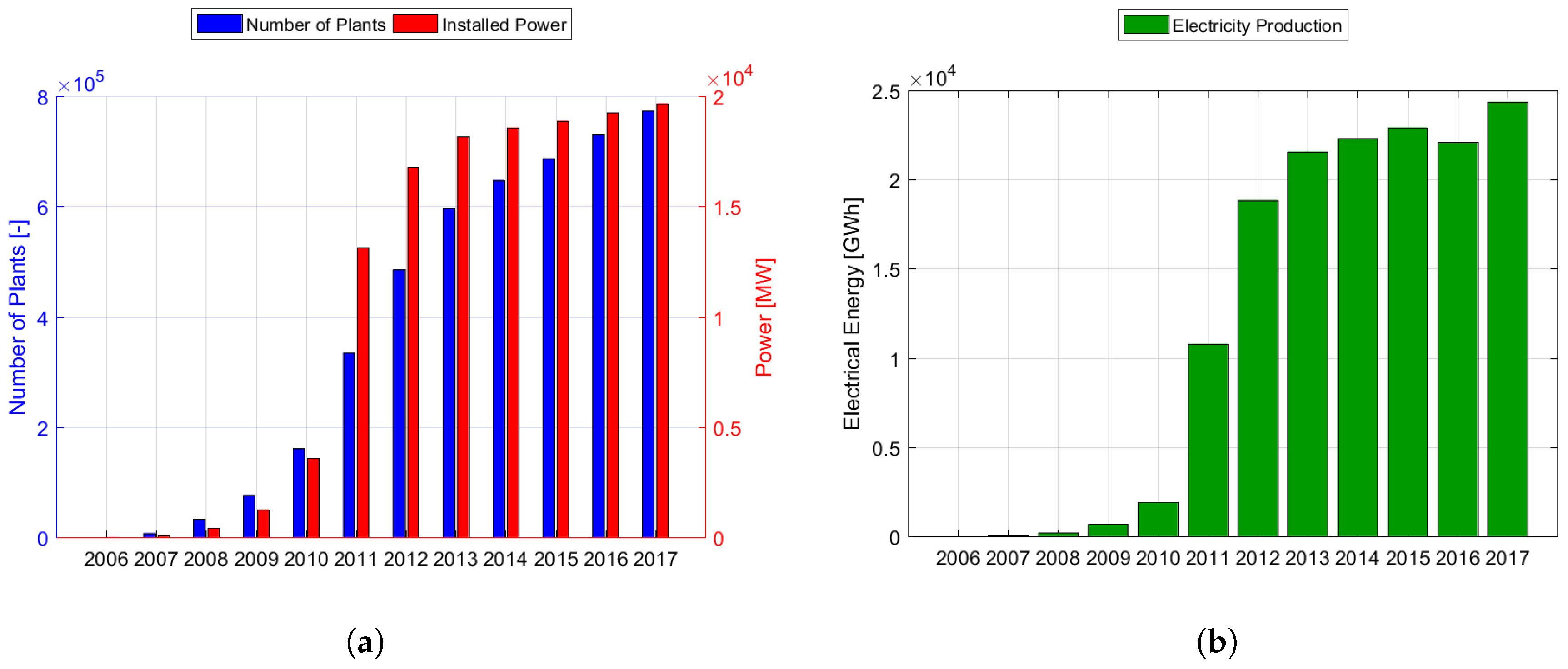
In 2006, there were 14 PV plants. In 2007, there were 7647, while in 2017, PV installations reached 774,014 units (see Figure 1a). In one year (2006–2007), there was a 54,500% increase, while in 10 years (2007–2017), the number of PV units increased by two orders of magnitude and now constitute over 90% of the net additions to power generation capacity [65,66].
In terms of installed power (see Figure 1a) and annual gross electricity production (see Figure 1b), the 10-year increment is also staggering. In 2007, the installed power was 86.80 MW, with an annual gross electricity production of 39.10 GWh, while 10 years later, installed power reached 19.682 GW with an annual gross electricity production of 24.378 TWh. This means that PV plants constitute about 20% of Italian installed power and can cover approximately 7% of the Italian electricity demand. The only issue is the reduction in the equivalent operating hours per year: 1200 [66].
Based on these data, it is possible to claim that in Italy there are a huge number of in-operation PV modules that can improve their electricity production and efficiency by means of cooling technologies, which is what prompts the authors to develop and test a low-cost and high-performance cooling system.
3. PV Test Rig Layout and Measurement Equipment
The PV cooling test rig is located in the Laboratory of Fluid Machines and Energy Systems in the Department of Industrial Engineering at the University of Padova. The facility is designed to test single or multiple PV modules equipped with or without a cooling system. Both active and passive cooling methods can be tested in the facility.
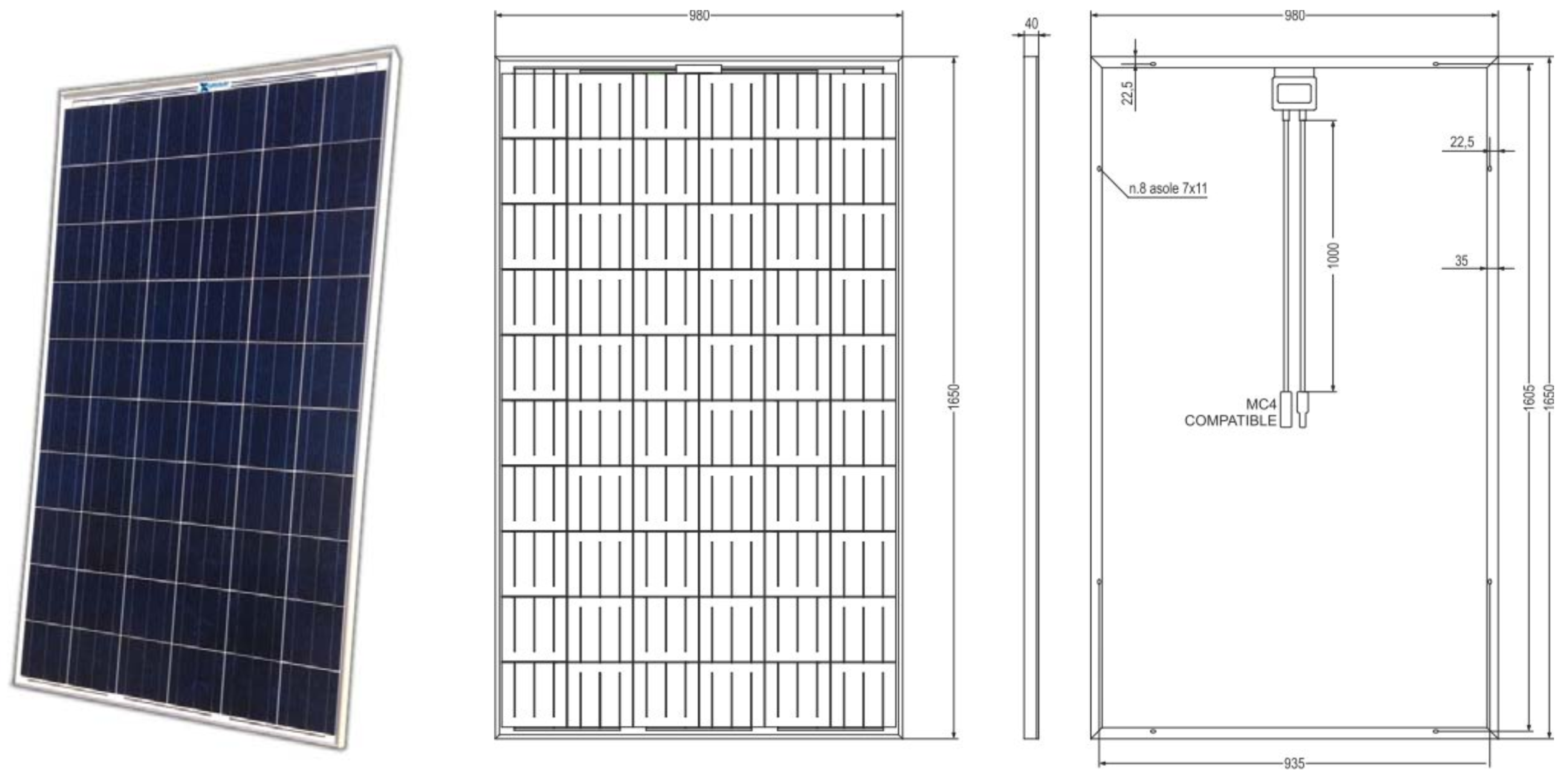
The proposed cooling system is applied to a commercially available flat PV monocrystalline module composed of 60 cells with a design power and an active surface equal to 230 W and 1.6 m, respectively. The module rating power voltage and current are 29.9 V and 7.68 A, respectively, while the open-circuit voltage and the short circuit current are 36.8 V and 8.34 A, respectively. The nominal operating cell (NOC) temperature is 45 C. Technical data refers to 25 C, a solar irradiance equal to 1000 W/m, and an air mass coefficient of 1.5, which is summarized in Table 7, while in Figure 2, the module geometrical dimensions are depicted.
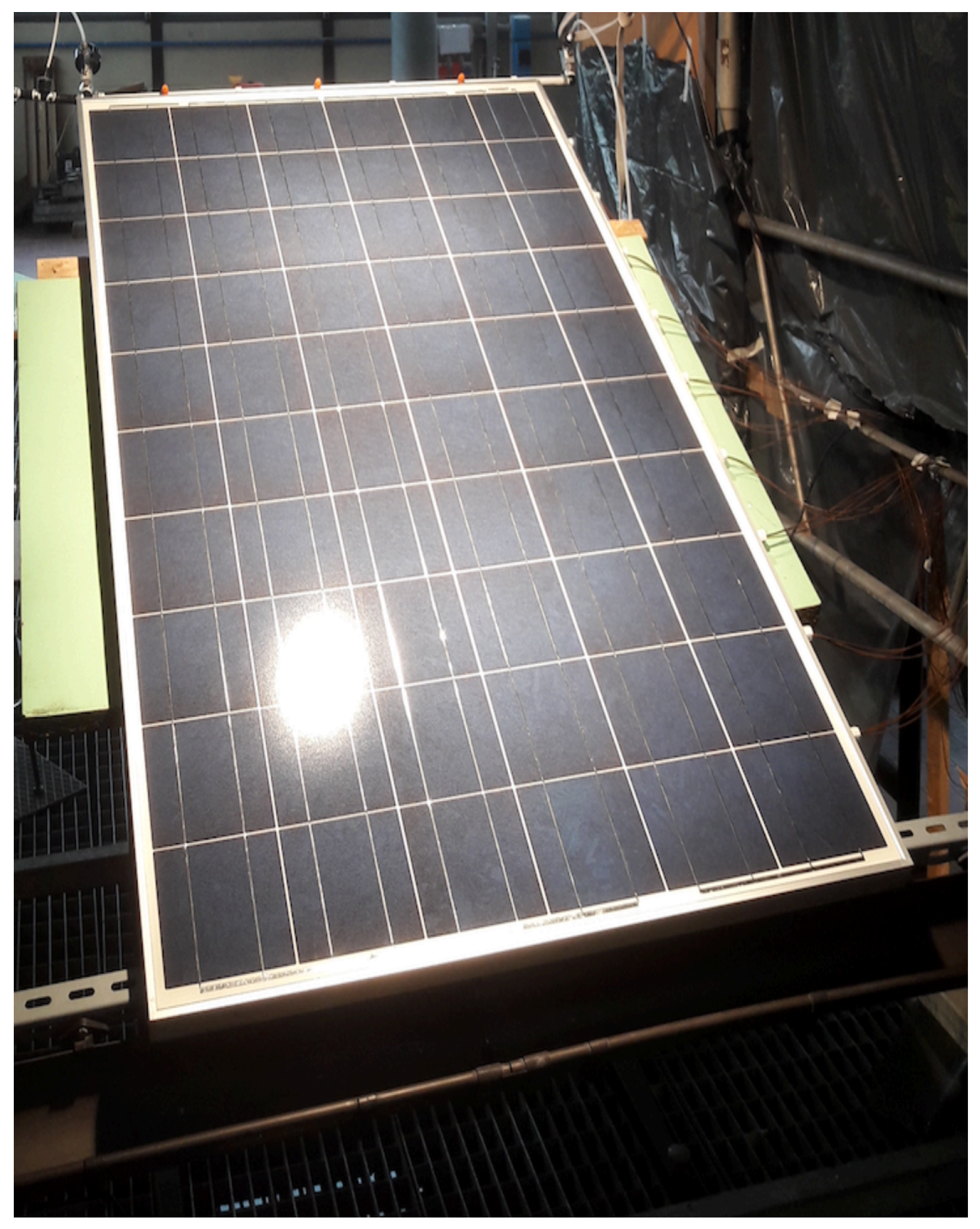
The PV module is located over a tilting desk as shown in Figure 3. The desk tilt angle can vary from 0 (perfectly horizontal) to 90 (perfectly vertical). Fixing the module on a rolling table allows us to set and test different tilt angles without dismantling the module, the cooling system, and the measurement apparatus. In the present work, the PV tilt angle is set to 30 because it is a conventional installation angle in Italy as stated in [66].
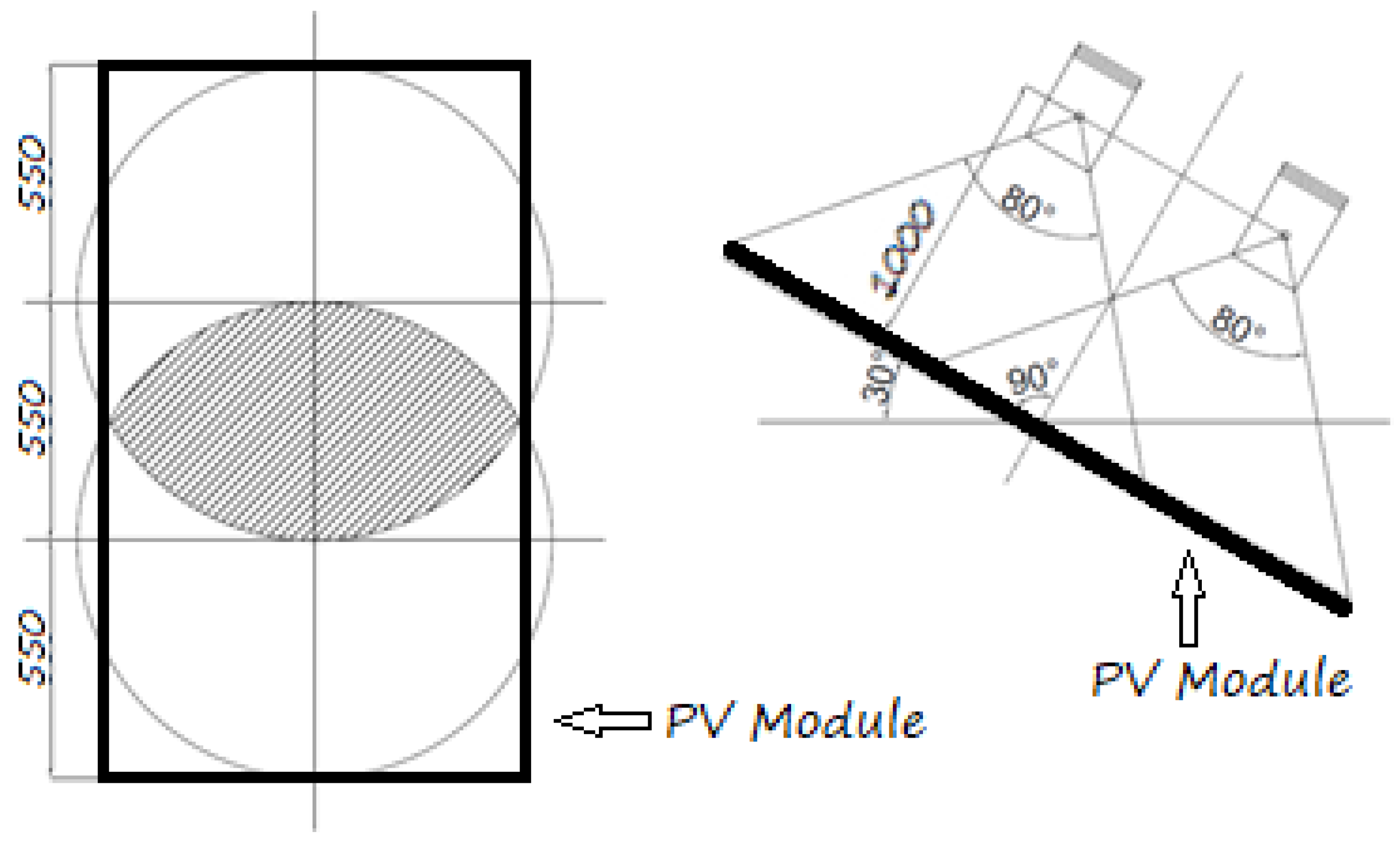
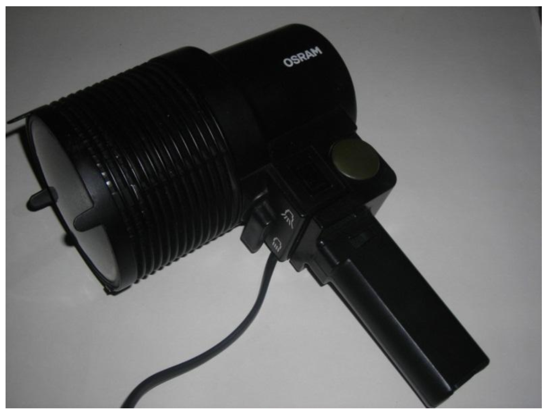
To simulate the solar radiation, two halogen lamps characterized by a design power of 1000 W, a lumen output of 33,000 lumen, and a color temperature of 3350 K, are installed over the PV module at a distance of 1 m each.
We performed experimental measurements on different days of the year under Padova’s climate conditions, and solar irradiance showed that adopting two lamps guarantees a realistic simulation of outdoor conditions in the laboratory test facility.
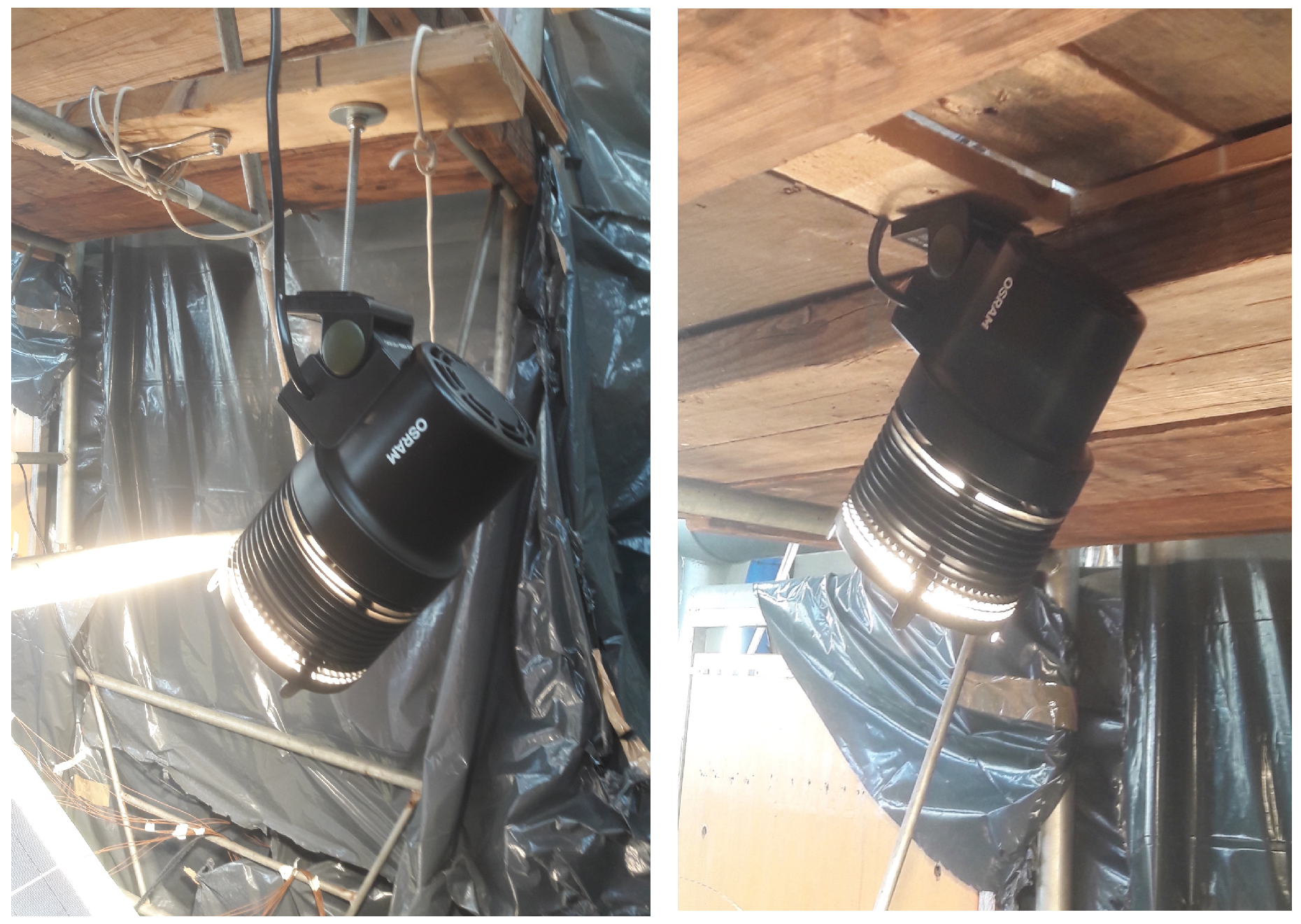
Figure 4 depicts the lamp illuminated area on the panel module surface and lamp inclination with respect to the module surface, while Figure 5 and Figure 6 show the adopted lamp model and the lamp installation position over the PV module.
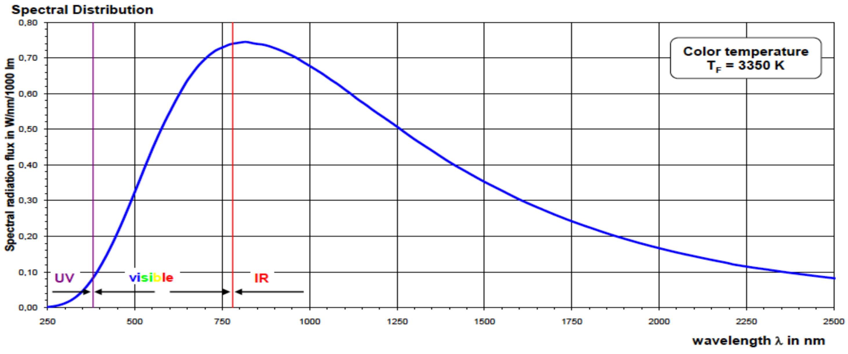
In Figure 7, the spectral distribution of the adopted lamp is reported. Comparing the lamp spectral distribution with the solar one, it is possible to observe that both display a maximum in the visible zone. Therefore, it is acceptable to adopt this type of lamp to simulate the sun effect on the module.
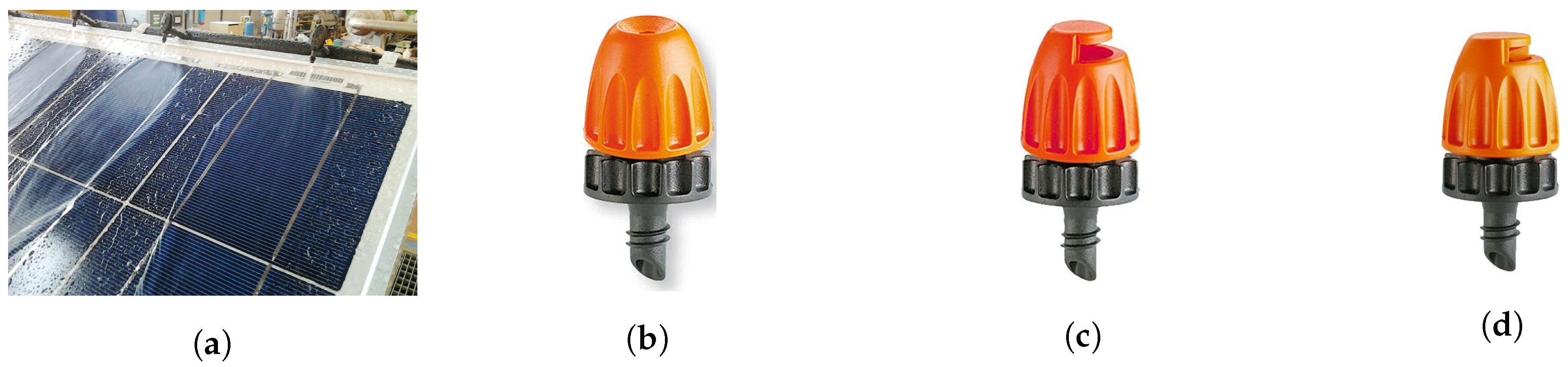
To minimize investment costs, the authors built the cooling system with a set of water nozzles initially designed for irrigation purposes (see Figure 8a). Nozzles are easy to find on the market, are available with a wide set of spraying angles (e.g., 90, 180, 360), are effortless to mount on water tubes, and are extremely durable. They contain features that guarantee to change the cooling arrangement in a few hours without extensively modify the test rig.
During the experimental campaign (as discussed in Section 4), the authors tested all the aforementioned spraying angles (90, 180, 360) but they found that the nozzle model at 90 is the best compromise between water consumption and film uniformity. For this reason, in Figure 8b, the authors demonstrate the 90 nozzle spray jet.
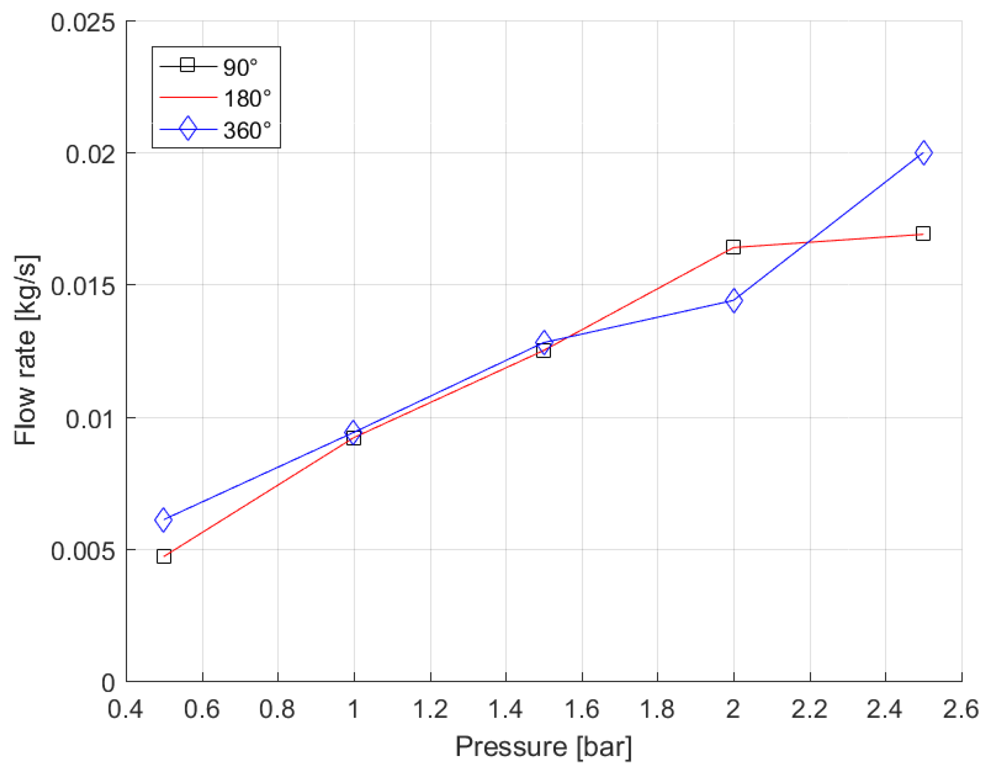
The adoption of this nozzle model guarantees to test several water flow rates while keeping the spraying angle constant, because flow rate is a function of nozzle inlet pressure. For example, Figure 9 depicts the 90, 180, and 360 nozzle inlet pressure vs. water mass flow rate characteristic.
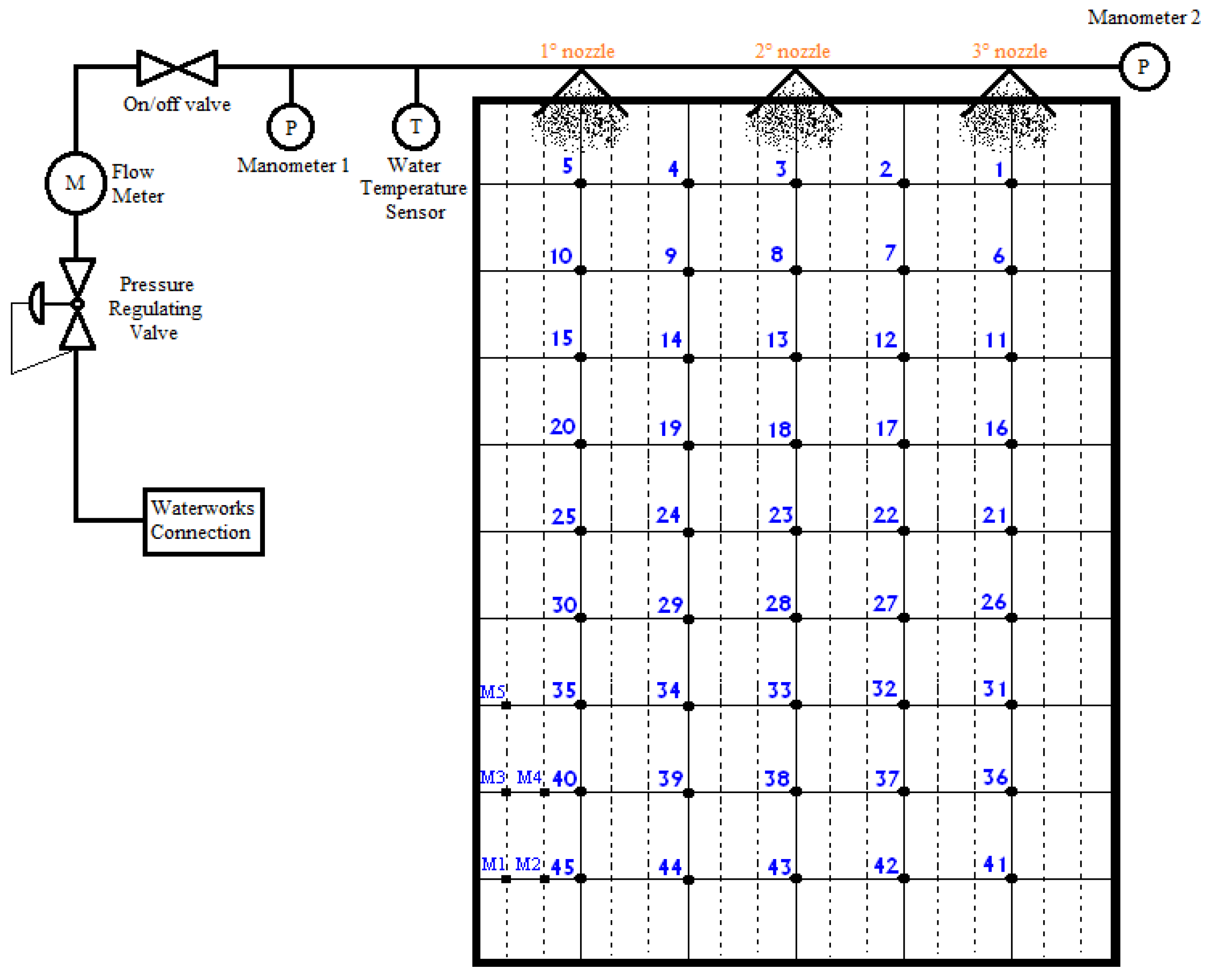
Nozzles are mounted on an orientable plastic pipe with a diameter of 20 mm (see, again, Figure 8b), and are fed by water taken from waterworks. Before the first nozzle and after the last one, two pressure gauges (manometer 1 and 2 in Figure 10) are mounted to measure nozzle inlet pressure and the pressure drop across the nozzles.
As mentioned above, the first aim of this work is to select the nozzle spraying angle but, after that, other work aims are the allocation of the nozzle number and their operating pressure, which guarantee the compromise between cooling efficiency and water consumption. As discussed in Section 4, the best compromise is a cooling system with 3 nozzles. For this reason, in Figure 10, the system is depicted with 3 water nozzles.
A T-type thermocouple is installed after manometer 1 to measure water temperature before it is sprayed on the panel. In the water circuit, a pressure-regulating valve, a flow meter, and an ON/OFF valve are mounted to control the water pressure, to measure the inlet mass flow rate and to start/stop the water flow during cooling cycles.
To monitor the panel surface temperature, 50 T-type thermocouples are stuck up on the back side of the module. Thermocouples are placed in cell intersections because this position is the best one for measuring module temperature distribution.
Thermocouples marked with symbol “M” are placed in a specific panel area where, during preliminary spraying tests, the authors observed non-cooled zones. Those thermocouple hotspots caused by non-uniform distribution of the water film can be detected.
Air temperature is measured by means of 3 T-type thermocouples: the first is placed between the module and the desk that supports it and measures the air temperature under the module; the second is located between the lamps and the PV panel to measure the temperature increment generated by the lamps (labeled in the Results section); and the third is placed in an unhindered zone of the laboratory to measure undisturbed room temperature.
Thermocouple error is ±0.3 C, while manometer error is ±0.01 bar.
The open-circuit voltage is measured using an “ad-hoc” National Instruments acquisition board. Data are acquired using an NI Modular DAQ system properly managed with an “in-house” acquisition code developed in the LabVIEW environment.
Data are collected with a frequency of 1 Hz and are then saved in a matrix, which is post-processed by means of an “in-house” code developed in MATLAB.
Valve opening and closing operations are also managed via an “in-house” code developed in LabVIEW.
4. Experimental Results
The first aim of the present experiment is the test of the nozzle performance in terms of water flow rate vs. spraying pressure. This step is mandatory since nozzles are commercially available devices designed for gardening purposes.
In gardening applications, the precision with which the water flow rate vs. spraying pressure curve is derived is still quite low, because the acceptable margin of error in the sprayed water at a certain pressure can reach ±25%. It is obvious that the incentive during the design of gardening nozzles is cost minimization, and not the accuracy in terms of sprayed water.
In conjunction with water flow rate vs. spraying pressure curve, it is also necessary to estimate the pressure drop across the nozzle, because this fundamental parameter is not provided by the nozzle manufacturer.
The characteristic curve of the nozzle with spraying angle of 90, 180, and 360 have been experimentally derived and compared with the manufacturer-provided curve. For the sake of compactness, only the 90 nozzle characteristic curve is presented and discussed.
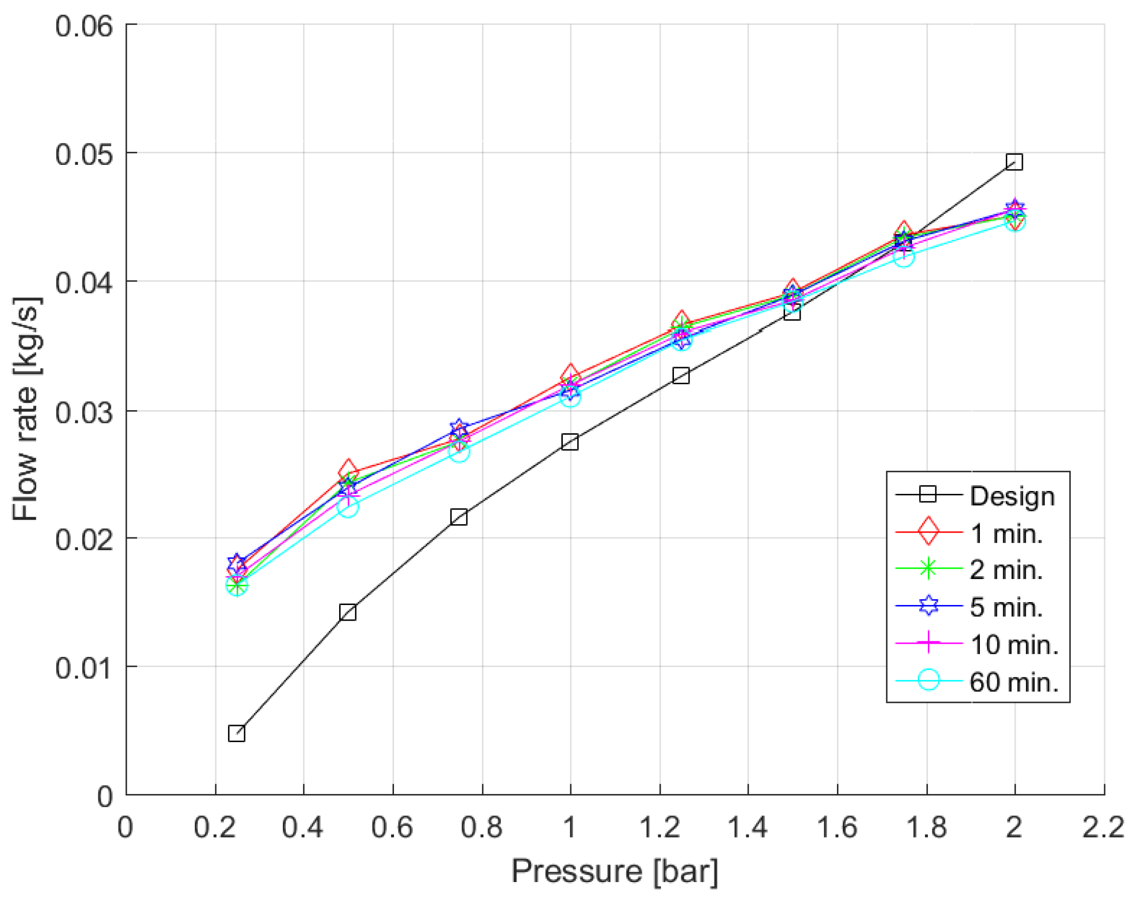
For each spraying pressure (0.25, 0.50, 0.75, 1.00, 1.25, 1.50, 1.75, and 2.00 bar), 3 nozzles (placed as depicted in Figure 10) are activated for 1, 2, 5, 10, and 60 min, and the sprayed water is collected in a water vessel. The collected water is weighed using a scale, and the water mass flow rate is computed. Then, the measured flow rate is compared with the one measured with the flow meter placed in the hydraulic water circuit.
Measuring the flow rate during different time periods is necessary for understanding the stability of the inlet spraying pressure and, consequently, of the flow coming from the waterworks. If tests demonstrated large instabilities or fluctuations in pressure or flow rate, the authors would have to develop a different water supply system.
The real flow rate is estimated using both flow meter and weight-control measure because, in this way, it is possible to estimate the mismatch between the two measurements. Results underline a difference of less than 1%.
Please note that during the spraying test on the PV module, the difference between the water measurement performed with the flow meter and weighing matches the water losses resulting from water evaporation and water flow that is sprayed outside of the PV panel.
Experimental measurements and data provided by the nozzle manufacturer are plotted in Figure 11 for 3 water nozzles with a sprayed angle of 90.
First, measured flow rates are grouped independently from the collection time. A discrepancy of less than 5% can be observed for measurements performed with different spraying time. This means that the water inlet pressure remains constant during a long spraying period (e.g., 60 min) as well as the sprayed flow rate. Both these outcomes are fundamental because they demonstrate both nozzle spraying accuracy and that water coming from the waterworks is at constant inlet pressure.
However, for pressures in the range 0.25–1.60 bar, the sprayed flow rate is higher than the declared one while for pressure in the range 1.75–2.00 bar, the flow rate is smaller than the designed one. At 0.25 bar, the measured flow rate is 3.8 times the designed one while, at 2.00 bar, the declared flow rate is 10% higher than the measured one. Around 1.6 bar, the discrepancy between the designed and measured values is less than 1%.
Concisely, comparisons among manufacturer data and the authors’ flow rate measurements show, independently of the spraying time, that design values are different from measurements. For this reason, the performed experimental campaign and its outcomes are crucial for properly estimating the water consumption of the proposed PV cooling arrangement.
Please note that spraying tests performed for different nozzles of the same type show mismatches in terms of sprayed water flow rate of lower than 1%. This means that despite the low nozzle costs, their manufacturing accuracy guarantees an acceptable mismatch in terms of flow rate.
Pressure measurements highlighted that the nozzle introduces a pressure drop of 0.033 bar independently to the nozzle inlet pressure. As for the water flow rate vs. spraying pressure curve, the performed test is a fundamental step because proper pressure drop estimations are essential when multiple nozzles are used. Since water flow rate is a function of pressure, when nozzles are placed in series, the total mass flow rate needs to be computed taking in account the real inlet pressure of each nozzle. As mentioned previously, the difference between flow meter measurements and the collected water at the bottom part of the module guarantees to compute water losses.
After the estimation of the flow rate vs. pressure characteristic curve and nozzle pressure drops, the authors studied the behavior of the nozzle’s sprayed water depending on the sprayed angle.
As shown in Figure 12a, the authors first tested a jet sprinkler and noticed that a water-cooling system with this type of jet is not able to generate a continuous film on the module surface. Then, they tested nozzles with different spraying angles: 360 (see, Figure 12b), 180 (see, Figure 12c), and 90 (see, Figure 12d).
Spraying tests demonstrate that independently of inlet pressure, using nozzles with 360 and 180 do not provoke, on the one hand, a uniform film on the PV module and, on the other hand, they introduce a loss of water greater than 30% and 50%, respectively.
Since nozzles are placed on the module upper part, the higher the spraying angle, the higher the flow rate that leaves the panel over the PV edges. For this reason, nozzles with a spraying angle of 360 and 180 can be a good solution in applications where multiple modules are arranged in rows.
Based on these remarks, the authors selected the nozzle with a spraying angle of 90 because it is the one that can establish a water film on the panel and reduce water losses over the PV module edges.
Regarding the number of nozzles installed on the upper part of the module, several tests are performed to identify the most suitable configuration.
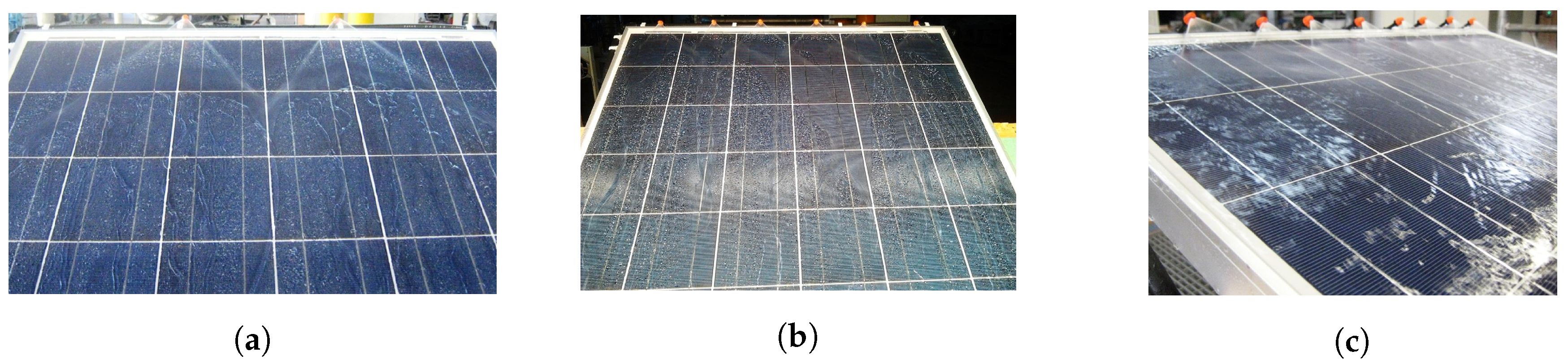
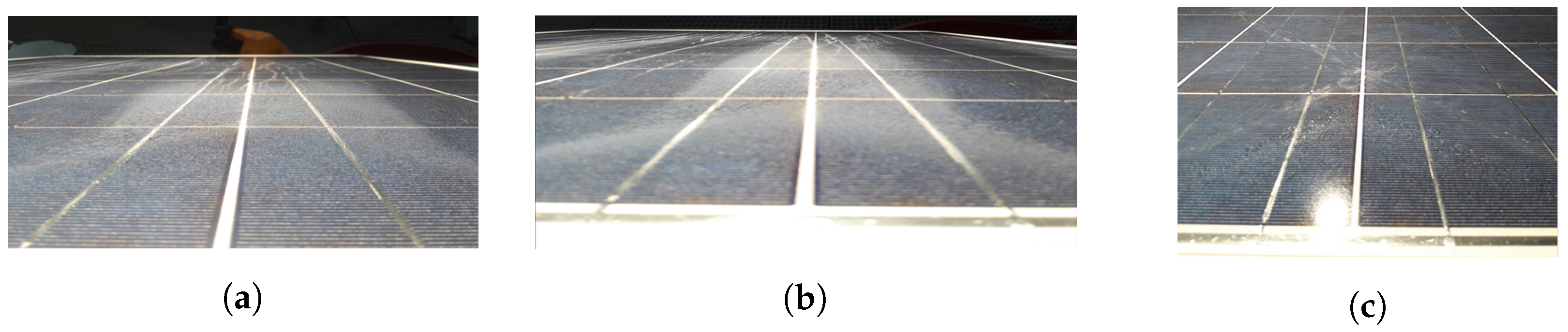
Spraying tests are performed with the number of nozzles varying between 1 and 9. Figure 13 depicts three spraying tests with 2, 6, and 9 water nozzles.
As shown in Figure 13a, two nozzles are unable to establish a uniform film on the panel surface and cool the upper part of the module, while 6 or 9 nozzles establish a very good water film, but the amount of water consumption is unacceptable. For this reason, and based on these tests, the authors stated that a good film can be established by adopting 3 nozzles located on the module upper part. This configuration also guarantees to reduce water losses along the module edges.
Further to previous points, it is worth remarking that 3 nozzles sprayed water at a pressure of 0.25 bar discharge 61 L/h while with an inlet pressure of 2.0 bar, water consumption becomes approximately 162 L/h. Given that the cooling system operates for at least 6 h per day during summer time, water consumptions per single PV module ranges between 368 L/day and 972 L/day. These values are unacceptable. For this reason, the authors developed a management strategy in which the cooling system operates with ON-OFF cycles. This strategy guarantees to reduce water and power consumption, but the main issue is to find the best ON-OFF time ratio.
For each water-pressure value (0.5, 1.0, 1.5, and 2.0 bar), the following cycles are tested: 30 s ON and 30 s OFF (30 s–30 s), 30 s–60 s, 30 s–120 s, 30 s–180 s, and 30 s–300 s.
As previously mentioned, the panel tilt angle is fixed to 30, the cooling system is equipped with 3 nozzles with a spraying angle of 90, and lamps are orthogonal to the panel, with their focus centered as depicted in Figure 4 and placed with a distance between the panel surface and each lamp focus equal to 1 m.
Cooling tests are performed after a PV module heating-up process as depicted in Figure 14.
In practice, the PV module is heated up by the two lamps until it reaches stability at maximum temperature. In this way, it is possible to observe the module’s temperature distribution. As clearly shown in Figure 14, the module temperature is not uniform.
Generally speaking, the PV module takes approximately 100–110 min to reach maximum temperature. Maximum temperature is observed at point 28 () and ranges from 74 C to 78 C, while the minimum one is detected at point M1 (T). The mean PV temperature after heating is 55–57 C, which means 32–37 C above the measured air temperature between the panel and the lamps. The mean heating rate is 0.33 C/min while the maximum and minimum, computed at points 28 and M1, are 0.45 C/min and 0.13 C/min, respectively. To be sure of reaching steady-state conditions, cooling cycles started after an additional 10–15 min.
Please note that water contained in the water pipe that feeds the nozzles is also subject to a temperature increase of 5–12 C. This aspect, as discussed below, affects the cooling system effectiveness during the early spraying cycles.
During both PV heating process and cooling cycles, temperatures and water distribution are symmetric. Then, taking into account Figure 10, at each second, the measured temperature, e.g., at point 1 (T) differs from the one observed at point 5 (T) by less than 1%. Similarly, T is approximately equal to T, and T is approximately the same as T. Subsequently, to limit the number of samples, only temperatures from the left of the PV module center are analyzed due to symmetry behavior of the temperature profiles.
As depicted in Figure 15a, adopting a water pressure of 0.5 bar does not allow a flow rate that can establish a water film on the module surface. The whole module is not fully wet, particularly in the bottom part (starting approximately from the horizontal line defined by points 26–30 in Figure 10). In fact, these thermocouples registered a small temperature decrease (10–20 C) compared to the ones placed in the upper part of the module (30–45 C). Therefore, this pressure is not enough to cool the PV module, because it does not guarantee a uniform film on the panel surface. Despite 0.5 bar guarantees to minimize water consumption, this pressure cannot be adopted with the selected nozzle configuration.
A water pressure of 1.0 bar is also inadequate for establishing a uniform film on the panel front surface. As shown in Figure 15b, the sprayed water is not able to cool the PV module zone in which thermocouples M1–M5 are located. A specular non-wet area is observed on the panel’s right side. Also, in the central part of the module (where thermocouples 38 and 43 are placed—Figure 10) the water film is not uniform, and only a small water streams is observed on the panel surface. As with the case of 0.5 bar, 1.0 bar is also not adequate for the proposed cooling system.
A uniform water film is given when the nozzle inlet pressure is 1.5 or 2.0 bar. However, spraying water at 2.0 bar instead of 1.5 bar increases water consumption and losses over the edges by 20% and 16%, respectively.
As depicted in Figure 15c, with 2.0 bar, water streams coming from the nozzles reach the module center (approximately concomitantly with points 21–25) and, since water is arriving at high velocity, part of the flow rate directly leaves the PV module surface from the right and the left module edge. Therefore, part of the water flow rate is lost. However, if the PV module is part of a module stream, this flow rate can be used to cool the module placed next to it. Therefore, in the future, experimental measurements with 2.0 bar will be performed using a stream of PV modules.
However, since the authors’ aim is to evaluate the cooling system performance in the case of a single PV module, the working pressure that guarantees a compromise between spraying uniformity, wet module area, water consumption, and water losses for the proposed configuration is 1.5 bar.
Therefore, in the following section, the authors analyze the temperature profile in the case of different ON/OFF cycles for a water-spraying pressure equal to 1.5 bar.
Figure 16 depicts temperature trends in the hottest and coldest point of the panel, the average PV surface temperature (T), and the air and the water temperatures for different ON/OFF cycles at a pressure of 1.5 bar.
During the heating process, the water contained in the adduction pipe increases in temperature by up to 5–12 C (see Figure 14). Therefore, during the first few spraying cycles, the water contained in the pipe is sprayed, and a new one, which is not subject to lamp flux, laps the water thermocouple. Thus, water temperature starts to decrease in the system.
Detecting water temperature increment caused by sunlight or, as in the present study, by lamps, is interesting because the higher the water temperature, the lower the cooling effect. In addition, the longer the OFF time, the longer the time required for water to reach waterworks temperature.
Please note that increasing OFF time from 30 to 300 s increases the time in which water remains in the tube before being sprayed. In fact, the comparison between the Figure 16a water temperature trend and the one depicted in Figure 16e clearly underlines that with 30 s–300 s ON/OFF cycles, water has time to warm up in the tube before being sprayed and, therefore, the cooling effect is reduced.
The detection of this important issue demonstrates the test rig’s capability of simulating the real system behavior because, in real applications, pipes that fed the cooling system are subject to sunlight. Therefore, the water temperature rises into pipes when the cooling system is turned off.
Adopting 30 s–30 s cycles (Figure 16a), the PV mean temperature reduction is equal to 35 C but requires 40 minutes to reach stability; with 30 s–300 s cycles (Figure 16e), the PV mean temperature reduction is equal to 22 C but it does not reach stability, and continues to cycle. Note that in Figure 16 the line markers are reduced (1 marker every 100–500 samples) to better depict temperature trends, but data are collected with a frequency of 1 Hz.
A switched-off period of 300 s instead of 30 s helps to reduce the sprayed water by 5 times, but as shown in Figure 16e, increases temperature fluctuations in both upper and lower parts of the module surface as well as the sprayed water one. In addition, during the 300 s in which the cooling system is switched off, a formation of limestone is observed on the module surface.
Similar temperature behavior is observed in the case of 30 s–180 s cycles. Therefore, 30 s–30 s, 30 s–180 s, and 30 s–300 s cycles are not suitable options because, in the first case, the water consumption is really high, while in second and third cases, limestone formations are observed.
The comparison between Figure 16b and Figure 16c shows PV mean temperature reduction equal to 29 C in the case of 30 s–60 s and of 28 C in the case of 30–120 s. Neither limestone formations on the module surface nor water temperature increase are observed. Therefore, these two cycles represent a good compromise between temperature reduction, film uniformity, and water consumption.
Considering a summer period in which the cooling system works in ON/OFF mode from 10 a.m. to 4 p.m., the sprayed water is reduced by 60% if 30–120 s cycle is adopted instead of 30–60 s cycles. Therefore, the best compromise for the proposed configuration is to adopt a spraying pressure of 1.5 bar and a 30 s–120 s ON/OFF cycle.
In terms of PV module efficiency, the proposed cooling system and management strategies guarantees to improve the efficiency from 12.2% to 13.9%. For a single module, the investment cost for pipes, nozzles, and support devices is lower than 15 €.
In this investigation, the authors consider feeding the system with water coming from waterworks but, in real applications, there is a need to adopt a pumping system. Regarding feed-pump consumption and management strategy, it is possible to claim that a pump cannot work for 30 s and then be off for 120 s, because this is not efficient. Therefore, to reduce pump energy consumption it is necessary to insert a pressurized water reservoir between the pump and the spraying system.
In this manner, the pump works only when the reservoir level drops under a certain level and stops pumping when the water tank is refilled. Obviously, in this case, the pump works at a higher efficiency than in the ON/OFF cycle mode, but its energy consumption depends on the water tank volume and the time to fill it.
Based on these remarks, at time of writing, the authors are working on a tank design and pump management optimization. Despite this aspect, preliminary calculations show that a water tank can reduce pump energy consumption by at least 30%.
Finally, it is also important to remark that the proposed active cooling system is, on the one hand, able to cool the module surface well, but on the other hand, still characterized by high water consumption. Therefore, additional investigations need to be done to additionally reduce the water usage in ground PV applications where the system can be easily applied in the present form to floating PV applications.
5. Conclusions
In the present work, the authors experimentally tested a low-cost PV module cooling system based on the sprayed water concept. Three water nozzles were placed in the upper part of the PV module. They are commercially available devices as well as connecting pipes and support devices. Water pressure and temperature, and air and PV module temperatures, were monitored using manometers and thermocouples directly managed with a LabVIEW code. Nozzle type and number, inlet nozzle pressure, and characteristic curve in terms of inlet spraying pressure vs. mass flow rate, as well as ON/OFF cycle ratio were the research findings.
Preliminary tests showed that nozzle characteristic curve in terms of inlet spraying pressure vs. flow rate differed from the manufacturer one. Nozzles with spraying angle of 180 and 360 were unable to establish a water film on the PV module surface while avoiding water losses over the module edges. Therefore, the first important result of the present investigation is the nozzle spraying angle needs to be 90.
After that, the number of nozzles that needs to be used was investigated. Results showed that a good compromise was guaranteed by 3 nozzles placed on the module upper part.
Subsequently, water-spraying pressures and five ON/OFF cycles were tested. Results demonstrated that a good compromise was reached using 1.5 bar as nozzle spraying pressure, and a 30 s–120 s ON/OFF cycle, because these settings guaranteed to reduce water consumption and improve PV efficiency from 12.2 to 13.9%. In addition, the investing cost for the cooling system is less than 15 € per single PV module.
Finally, it is possible to claim that the proposed water-spray cooling technique can potentially increase the PV panel performance due to an evaporation and self-cleaning effect, which is of great benefit in PV applications.
In addition, this type of cooling system can be easily applied to floating PV installations because, in that case, the water consumption is not an issue since PV modules are located on lake, sea, or river surface. The cooling water is sucked from, e.g., the lake and, after it cools the module, it returns to the lake. No water is wasted and, since water mixing is established, this helps to introduce more oxygen into the water.
Obviously, more investigations need to be performed to estimate pump consumptions and establish whether the benefit in terms of additional PV production is higher than the energy consumed by the pumping system.
Author Contributions
Conceptualization, A.B. and A.S.; Data curation, A.B. and A.S.; Investigation, A.B. and A.S.; Methodology, A.B. and A.S.; Writing—original draft, A.B.; Writing—review & editing, A.B. and A.S.
Funding
This research received no external funding.
Conflicts of Interest
The authors declare no conflict of interest.
Abbreviations
The following abbreviations are used in this manuscript:
| AlO | Aluminum Oxide |
| bil US$ | billion of US Dollars |
| CdTe | Cadmium Telluride |
| CO | Carbon Dioxide |
| CIGS | copper indium gallium (di) selenide |
| CuO | Copper(II) oxide |
| P | Electrical Power |
| EU | European Union |
| GSE | Gestore Servizi Energetici |
| GHG | Greenhouse Gases |
| GDP | Gross Domestic Product |
| NREAP | National Renewable Energy Action Plan |
| NOC | Nominal Operating Cell |
| OECD | Organization for Economic Co-operation and Development |
| PCM | Phase Change Material |
| PV | Photovoltaic |
| RES | Renewable Energy Sources |
| vs. | versus |
References
- International Monetary Found. World Economic Outlook (October 2018). 2018. Available online: https://www.imf.org/external/datamapper/NGDP_RPCH@WEO/OEMDC/ADVEC/WEOWORLD (accessed on 15 January 2019).
- BP. BP Statistical Review of World Energy 2018. 2018. Available online: https://www.bp.com/en/global/corporate/energy-economics/statistical-review-of-world-energy. html (accessed on 15 January 2019).
- Grubb, M.; Vrolijk, C.; Brack, D. The Kyoto Protocol: A Guide and Assessment; Royal Institute of International Affairs, Energy and Environmental Programme: London, UK, 1997. [Google Scholar]
- The Paris Agreement. United Nations Framework Convention on Climate Change; The Paris Agreement: Paris, France, 2015. [Google Scholar]
- European Parliament and Council of the European Union. Directive 2009/28/EC of the European Parliament and of the Council of 23 April 2009 on the Promotion of the Use of Energy From Renewable Sources and Amending and Subsequently Repealing Directives 2001/77/EC and 2003/30/EC. 2009. Available online: https://eur-lex.europa.eu/LexUriServ/LexUriServ.do?uri=OJ:L:2009:140:0016:0062:en:PDF (accessed on 15 January 2019).
- European Parliament and Council of the European Union. 2030 Framework for Climate and Energy Policies. 2014. Available online: www.ec.europa.eu (accessed on 15 January 2019).
- European Climate Foundation. EU Roadmap 2050. 2010. Available online: www.roadmap2050.eu (accessed on 15 January 2019).
- Italian Governament. National Renewable Energy Action Plan. 2010. Available online: https://ec.europa.eu/energy/en/topics/renewable-energy/national-action-plans (accessed on 15 January 2019).
- International Energy Agency. Italian National Renewable Energy Action Plan. 2010. Available online: https://www.iea.org/policiesandmeasures/pams/italy/name-39509-en.php (accessed on 15 January 2019).
- Benato, A.; Stoppato, A. Pumped Thermal Electricity Storage: A technology overview. Therm. Sci. Eng. Prog. 2018, 6, 301–315. [Google Scholar] [CrossRef]
- Benato, A.; Stoppato, A. Energy and cost analysis of an Air Cycle used as prime mover of a Thermal Electricity Storage. J. Energy Storage 2018, 17, 29–46. [Google Scholar] [CrossRef]
- Benato, A.; Stoppato, A. Heat transfer fluid and material selection for an innovative Pumped Thermal Electricity Storage system. Energy 2018, 147, 155–168. [Google Scholar] [CrossRef]
- Benato, A.; Stoppato, A. Energy and Cost Analysis of a New Packed Bed Pumped Thermal Electricity Storage Unit. J. Energy Resour. Technol. 2018, 140, 020904. [Google Scholar] [CrossRef]
- Park, H.; Baldick, R. Integration of compressed air energy storage systems co-located with wind resources in the ERCOT transmission system. Int. J. Electr. Power Energy Syst. 2017, 90, 181–189. [Google Scholar] [CrossRef]
- Benato, A. Performance and cost evaluation of an innovative Pumped Thermal Electricity Storage power system. Energy 2017, 138, 419–436. [Google Scholar] [CrossRef]
- Benato, A.; Stoppato, A.; Mirandola, A. State-of-the-art and future development of sensible heat thermal electricity storage systems. Int. J. Heat Technol. 2017, 35, 244–251. [Google Scholar] [CrossRef]
- Teo, H.; Lee, P.; Hawlader, M.N.A. An active cooling system for photovoltaic modules. Appl. Energy 2012, 90, 309–315. [Google Scholar] [CrossRef]
- Fraunhofer Institute for Solar Energy Systems, ISE. Photovoltaics Report. 2019. Available online: https://www.ise.fraunhofer.de/content/dam/ise/de/documents/publications/studies/Photovoltaics-Report.pdf (accessed on 15 March 2019).
- What Are the Most Efficient Solar Panels on the Market? 2019. Available online: https://news.energysage.com/what-are-the-most-efficient-solar-panels-on-the-market/ (accessed on 15 January 2019).
- Skoplaki, E.; Palyvos, J. On the temperature dependence of photovoltaic module electrical performance: A review of efficiency/power correlations. Sol. Energy 2009, 83, 614–624. [Google Scholar] [CrossRef]
- Shan, F.; Tang, F.; Cao, L.; Fang, G. Comparative simulation analyses on dynamic performances of photovoltaic–thermal solar collectors with different configurations. Energy Convers. Manag. 2014, 87, 778–786. [Google Scholar] [CrossRef]
- Rahman, M.; Hasanuzzaman, M.; Rahim, N. Effects of various parameters on PV-module power and efficiency. Energy Convers. Manag. 2015, 103, 348–358. [Google Scholar] [CrossRef]
- Sargunanathan, S.; Elango, A.; Mohideen, S.T. Performance enhancement of solar photovoltaic cells using effective cooling methods: A review. Renew. Sustain. Energy Rev. 2016, 64, 382–393. [Google Scholar] [CrossRef]
- Nižetić, S.; Grubišić-Čabo, F.; Marinić-Kragić, I.; Papadopoulos, A.M. Experimental and numerical investigation of a backside convective cooling mechanism on photovoltaic panels. Energy 2016, 111, 211–225. [Google Scholar] [CrossRef]
- Safi, T.S.; Munday, J.N. Improving photovoltaic performance through radiative cooling in both terrestrial and extraterrestrial environments. Opt. Express 2015, 23, A1120–A1128. [Google Scholar] [CrossRef] [PubMed]
- Moharram, K.A.; Abd-Elhady, M.; Kandil, H.; El-Sherif, H. Enhancing the performance of photovoltaic panels by water cooling. Ain Shams Eng. J. 2013, 4, 869–877. [Google Scholar] [CrossRef] [Green Version]
- Nižetić, S.; Čoko, D.; Yadav, A.; Grubišić-Čabo, F. Water spray cooling technique applied on a photovoltaic panel: The performance response. Energy Convers. Manag. 2016, 108, 287–296. [Google Scholar] [CrossRef]
- Zsiborács, H.; Pályi, B.; Pintér, G.; Popp, J.; Balogh, P.; Gabnai, Z.; Pető, K.; Farkas, I.; Baranyai, N.H.; Bai, A. Technical-economic study of cooled crystalline solar modules. Sol. Energy 2016, 140, 227–235. [Google Scholar] [CrossRef] [Green Version]
- Alami, A.H. Effects of evaporative cooling on efficiency of photovoltaic modules. Energy Convers. Manag. 2014, 77, 668–679. [Google Scholar] [CrossRef]
- Rahimi, M.; Valeh-e Sheyda, P.; Parsamoghadam, M.A.; Masahi, M.M.; Alsairafi, A.A. Design of a self-adjusted jet impingement system for cooling of photovoltaic cells. Energy Convers. Manag. 2014, 83, 48–57. [Google Scholar] [CrossRef]
- Ebrahimi, M.; Rahimi, M.; Rahimi, A. An experimental study on using natural vaporization for cooling of a photovoltaic solar cell. Int. Commun. Heat Mass Transf. 2015, 65, 22–30. [Google Scholar] [CrossRef]
- Zhang, Y.; Du, Y.; Shum, C.; Cai, B.; Le, N.C.H.; Chen, X.; Duck, B.; Fell, C.; Zhu, Y.; Gu, M. Efficiently-cooled plasmonic amorphous silicon solar cells integrated with a nano-coated heat-pipe plate. Sci. Rep. 2016, 6, 24972. [Google Scholar] [CrossRef] [Green Version]
- Bai, A.; Popp, J.; Balogh, P.; Gabnai, Z.; Pályi, B.; Farkas, I.; Pintér, G.; Zsiborács, H. Technical and economic effects of cooling of monocrystalline photovoltaic modules under Hungarian conditions. Renew. Sustain. Energy Rev. 2016, 60, 1086–1099. [Google Scholar] [CrossRef] [Green Version]
- Sato, D.; Yamada, N. Review of photovoltaic module cooling methods and performance evaluation of the radiative cooling method. Renew. Sustain. Energy Rev. 2019, 104, 151–166. [Google Scholar] [CrossRef]
- Ahmad, N.; Khandakar, A.; El-Tayeb, A.; Benhmed, K.; Iqbal, A.; Touati, F. Novel Design for Thermal Management of PV Cells in Harsh Environmental Conditions. Energies 2018, 11, 3231. [Google Scholar] [CrossRef]
- Siecker, J.; Kusakana, K.; Numbi, B. A review of solar photovoltaic systems cooling technologies. Renew. Sustain. Energy Rev. 2017, 79, 192–203. [Google Scholar] [CrossRef]
- Prudhvi, P.; Sai, P.C. Efficiency improvement of solar PV panels using active cooling. In Proceedings of the 2012 11th International Conference on Environment and Electrical Engineering (EEEIC), Venice, Italy, 18–25 May 2012; pp. 1093–1097. [Google Scholar]
- Krauter, S. Increased electrical yield via water flow over the front of photovoltaic panels. Sol. Energy Mater. Sol. Cells 2004, 82, 131–137. [Google Scholar] [CrossRef]
- Hasanuzzaman, M.; Malek, A.; Islam, M.; Pandey, A.; Rahim, N. Global advancement of cooling technologies for PV systems: A review. Sol. Energy 2016, 137, 25–45. [Google Scholar] [CrossRef]
- Chandrasekar, M.; Suresh, S.; Senthilkumar, T.; Ganesh Karthikeyan, M. Passive cooling of standalone flat PV module with cotton wick structures. Energy Convers. Manag. 2013, 71, 43–50. [Google Scholar] [CrossRef]
- Reddy, S.R.; Ebadian, M.A.; Lin, C.X. A review of PV–T systems: Thermal management and efficiency with single phase cooling. Int. J. Heat Mass Transf. 2015, 91, 861–871. [Google Scholar] [CrossRef]
- Baloch, A.A.; Bahaidarah, H.M.; Gandhidasan, P.; Al-Sulaiman, F.A. Experimental and numerical performance analysis of a converging channel heat exchanger for PV cooling. Energy Convers. Manag. 2015, 103, 14–27. [Google Scholar] [CrossRef]
- Rahimi, M.; Asadi, M.; Karami, N.; Karimi, E. A comparative study on using single and multi header microchannels in a hybrid PV cell cooling. Energy Convers. Manag. 2015, 101, 1–8. [Google Scholar] [CrossRef]
- Skovajsa, J.; Koláček, M.; Zálešák, M. Phase change material based accumulation panels in combination with renewable energy sources and thermoelectric cooling. Energies 2017, 10, 152. [Google Scholar] [CrossRef]
- Kim, J.; Nam, Y. Study on the Cooling Effect of Attached Fins on PV Using CFD Simulation. Energies 2019, 12, 758. [Google Scholar] [CrossRef]
- Brinkworth, B. Estimation of flow and heat transfer for the design of PV cooling ducts. Sol. Energy 2000, 69, 413–420. [Google Scholar] [CrossRef]
- Odeh, S.; Behnia, M. Improving photovoltaic module efficiency using water cooling. Heat Transf. Eng. 2009, 30, 499–505. [Google Scholar] [CrossRef]
- Tonui, J.; Tripanagnostopoulos, Y. Improved PV/T solar collectors with heat extraction by forced or natural air circulation. Renew. Energy 2007, 32, 623–637. [Google Scholar] [CrossRef]
- Nižetić, S.; Papadopoulos, A.; Giama, E. Comprehensive analysis and general economic-environmental evaluation of cooling techniques for photovoltaic panels, Part I: Passive cooling techniques. Energy Convers. Manag. 2017, 149, 334–354. [Google Scholar] [CrossRef]
- Nižetić, S.; Giama, E.; Papadopoulos, A. Comprehensive analysis and general economic-environmental evaluation of cooling techniques for photovoltaic panels, Part II: Active cooling techniques. Energy Convers. Manag. 2018, 155, 301–323. [Google Scholar] [CrossRef]
- Schiro, F.; Benato, A.; Stoppato, A.; Destro, N. Improving photovoltaics efficiency by water cooling: Modelling and experimental approach. Energy 2017, 137, 798–810. [Google Scholar] [CrossRef]
- Benato, A.; Macor, A. Italian Biogas Plants: Trend, Subsidies, Cost, Biogas Composition and Engine Emissions. Energies 2019, 12, 979. [Google Scholar] [CrossRef]
- Serri, L.; Lembo, E.; Airoldi, D.; Gelli, C.; Beccarello, M. Wind energy plants repowering potential in Italy: technical-economic assessment. Renew. Energy 2018, 115, 382–390. [Google Scholar] [CrossRef]
- European Parliament and Council of the European Union. Directive 2001/77/EC of the European Parliament and Council of the European Union of 27 September 2001 on the Promotion of Electricity Produced from Renewable Energy Sources in the Internal Electricity Market. 2001. Available online: https://eur-lex.europa.eu/legal-content/EN/TXT/?uri=CELEX%3A32001L0077 (accessed on 15 March 2019).
- Italian Government. Decreto Legislativo 29 Dicembre 2003. Attuazione della Direttiva 2001/77/CE Relativa Alla Promozione Dell’energia Elettrica Prodotta da Fonti Energetiche Rinnovabili Nel Mercato Interno Dell’elettricita. 2003. Available online: https://www.gse.it/documenti_site/Documenti%20GSE/Servizi%20per%20te/CONTO%20ENERGIA/Normativa/_D.LGS+29122003+N.+387.PDF (accessed on 15 January 2019).
- Italian Government. Decreto 28 Luglio 2005. Criteri per L’incentivazione Della Produzione di Energia Elettrica Mediante Conversione Fotovoltaica Della Fonte Solare. 2005. Available online: https://www.ambientediritto.it/Legislazione/Energia/2005/dm%2028lug2005.htm (accessed on 15 January 2019).
- Italian Government. Decreto 6 Febbraio 2006. Criteri per L’incentivazione Della Produzione di Energia Elettrica Mediante Conversione Fotovoltaica Della Fonte Solare. 2006. Available online: https://www.ambientediritto.it/Legislazione/Energia/2006/dm_6feb2006.htm (accessed on 15 January 2019).
- Italian Government. Decreto 19 Febbraio 2007. Criteri E Modalita Per Incentivare La Produzione di Energia Elettrica Mediante Conversione Fotovoltaica Della Fonte Solare, in Attuazione Dell’articolo 7 del Decreto Legislativo 29 Dicembre 2003, N. 387. 2007. Available online: http://efficienzaenergetica.acs.enea.it/doc/decreto_fotovoltaico.pdf (accessed on 15 January 2019).
- Scerrato, G. Solar PV Feed-In Tariff: the Distortion of Italian Power Market. 2015. Available online: http://www.summerschool-aidi.it/edition-2015/images/Naples2015/proceed/30_scerrato.pdf (accessed on 15 January 2019).
- Italian Government. Decreto Ministeriale 6 Agosto 2010. Incentivazione Della Produzione di Energia Elettrica Mediante Conversione Fotovoltaica Della Fonte Solare. 2010. Available online: https://energia.regione.emilia-romagna.it/leggi-atti-bandi-1/norme-e-atti-amministrativi/fonti-rinnovabili/nazionale/decreto%20ministeriale%206%20%20agosto%202010.pdf (accessed on 15 January 2019).
- Italian Government. Decreto Ministeriale 5 Maggio 2011. Incentivazione Della Produzione di Energia Elettrica da Impianti Solari Fotovoltaici. 2011. Available online: http://www.energia.provincia.tn.it/binary/pat_agenzia_energia/normativa/D.M._5_5_2011_Quarto_c._energia.1306333464.pdf (accessed on 15 January 2019).
- Italian Government. Decreto Legislativo 3 Marzo 2011, N. 28. Attuazione Della Direttiva 2009/28/CE Sulla Promozione Dell’uso Dell’energia da Fonti Rinnovabili, Recante Modifica e Successiva Abrogazione Delle Direttive 2001/77/CE e 2003/30/CE. 2011. Available online: http://www.acs.enea.it/doc/dlgs_28-2011.pdf (accessed on 15 January 2019).
- Italian Government. Decreto 5 Luglio 2012 Attuazione Dell’art. 25 Del Decreto Legislativo 3 Marzo 2011, N. 28, Recante Incentivazione Della Produzione di Energia Elettrica da Impianti Solari Fotovoltaici (c.d. Quinto Conto Energia). (12A07629) (GU Serie Generale n.159 del 10-07-2012—Suppl. Ordinario n. 143). 2012. Available online: http://www.arpa.veneto.it/temi-ambientali/energia/file-e-allegati/normativa/DM_5_luglio2012_quinto_conto_energia.pdf (accessed on 15 January 2019).
- Gestore dei Servizi Elettrici. Ritiro Dedicato. 2019. Available online: https://www.gse.it/servizi-per-te/fotovoltaico/ritiro-dedicato/tariffe-e-copertura-del-servizio (accessed on 15 March 2019).
- Terna. Dati Statistici. 2017. Available online: https://www.terna.it/it-it/sistemaelettrico/statisticheeprevisioni/datistatistici.aspx (accessed on 15 September 2018).
- Gestore dei Servizi Energetici S.p.A. Rapporto Statistico Solare Fotovoltaico 2017. 2018. Available online: https://www.gse.it/dati-e-scenari/statistiche (accessed on 15 September 2018).
- Osram. SLV1000. Available online: https://www.osram.it/cb/index.jsp (accessed on 15 March 2019).
- Claber. MicroirrigatoriRainjet per i Sistemi a Goccia. Available online: https://www.claber.com/it/prodotti/irrigazione-a-goccia/irrigazione-goccia-elenco.asp?fm=51 (accessed on 15 March 2019).
Figure 1.
Trend of Italian PV (a) installed power and number of plants, (b) generated electricity. Source: [66].
Figure 1.
Trend of Italian PV (a) installed power and number of plants, (b) generated electricity. Source: [66].

Figure 2.
PV module dimensions in millimeters.

Figure 3.
PV module installation. The module is fixed on a tilting desk.

Figure 4.
Lamp illuminated area on the panel module surface (left) and lamp inclination with respect to module surface (right). Dimensions are expressed in millimeters.
Figure 4.
Lamp illuminated area on the panel module surface (left) and lamp inclination with respect to module surface (right). Dimensions are expressed in millimeters.

Figure 5.
Adopted lamp: Osram SLV1000 (by courtesy of [67]).
Figure 5.
Adopted lamp: Osram SLV1000 (by courtesy of [67]).

Figure 6.
Lamp installation position over the PV module.

Figure 7.
Lam spectral distribution. By courtesy of [67].
Figure 7.
Lam spectral distribution. By courtesy of [67].

Figure 8.
(a) Nozzle used to spray the water, (b) 90 nozzle spraying angle. By courtesy of [68].
Figure 8.
(a) Nozzle used to spray the water, (b) 90 nozzle spraying angle. By courtesy of [68].

Figure 9.
Inlet pressure vs. water mass flow rate characteristic for one nozzle with a spraying angle of 90, 180 and 360. By courtesy of [68].
Figure 9.
Inlet pressure vs. water mass flow rate characteristic for one nozzle with a spraying angle of 90, 180 and 360. By courtesy of [68].

Figure 10.
Hydraulic water circuit and thermocouples position on the PV module. Numbers refer to thermocouple name and position on the PV module.
Figure 10.
Hydraulic water circuit and thermocouples position on the PV module. Numbers refer to thermocouple name and position on the PV module.

Figure 11.
Measured and design flow rate sprayed from 3 nozzles with a sprayed angle of 90 and placed as depicted in Figure 10.
Figure 11.
Measured and design flow rate sprayed from 3 nozzles with a sprayed angle of 90 and placed as depicted in Figure 10.

Figure 12.
(a) Jet sprinkler, (b) Nozzle with 360 of spraying angle, (c) Nozzle with 180 of spraying angle, (d) Nozzle with 90 of spraying angle. By courtesy of [68].
Figure 12.
(a) Jet sprinkler, (b) Nozzle with 360 of spraying angle, (c) Nozzle with 180 of spraying angle, (d) Nozzle with 90 of spraying angle. By courtesy of [68].

Figure 13.
Spraying test with (a) 2 water nozzles, (b) 6 water nozzles, (c) 9 water nozzles.

Figure 14.
PV module heating-up process. Temperature trends of air, water, and PV module points during heating process.
Figure 14.
PV module heating-up process. Temperature trends of air, water, and PV module points during heating process.

Figure 15.
Water maldistribution on PV module with a spraying pressure of (a) 0.5 bar, (b) 1.0 bar and (c) 2.0 bar.
Figure 15.
Water maldistribution on PV module with a spraying pressure of (a) 0.5 bar, (b) 1.0 bar and (c) 2.0 bar.

Figure 16.
Trends of air, water, and PV module point temperatures during (a) 30 s–30 s, (b) 30 s–60 s, (c) 30 s–120 s, (d) 30 s–180 s, and (e) 30 s–300 s cycles.
Figure 16.
Trends of air, water, and PV module point temperatures during (a) 30 s–30 s, (b) 30 s–60 s, (c) 30 s–120 s, (d) 30 s–180 s, and (e) 30 s–300 s cycles.


Table 1.
Standard feed-in tariff established in [63].
Table 1.
Standard feed-in tariff established in [63].
| Size | Rooftop Incentive | Ground-Mounted | Term |
|---|---|---|---|
| [€/MWh] | [€/MWh] | [years] | |
| 1–3 kW | 182 | 176 | 20 |
| 3–20 kW | 171 | 165 | 20 |
| 20–200 kW | 157 | 151 | 20 |
| 200 kW–1 MW | 130 | 124 | 20 |
| 1 MW–5 MW | 118 | 113 | 20 |
| >5 MW | 112 | 106 | 20 |
Table 2.
Standard self-consumption tariff established in [63].
Table 2.
Standard self-consumption tariff established in [63].
| Size | Rooftop Incentive | Ground-Mounted | Term |
|---|---|---|---|
| [€/MWh] | [€/MWh] | [years] | |
| 1–3 kW | 100 | 94 | 20 |
| 3–20 kW | 89 | 83 | 20 |
| 20–200 kW | 75 | 69 | 20 |
| 200 kW–1 MW | 48 | 42 | 20 |
| 1 MW–5 MW | 36 | 31 | 20 |
| >5 MW | 30 | 24 | 20 |
Table 3.
Standard tariffs for PV plants using innovative technology established in [63].
Table 3.
Standard tariffs for PV plants using innovative technology established in [63].
| Size | Incentive | Term |
|---|---|---|
| [€/MWh] | [years] | |
| 1–20 kW | 240 | 20 |
| 20–200 kW | 231 | 20 |
| >200 kW * | 217 | 20 |
Table 4.
Self-consumption tariffs for PV plants using innovative technology established in [63].
Table 4.
Self-consumption tariffs for PV plants using innovative technology established in [63].
| Size | Incentive | Term |
|---|---|---|
| [€/MWh] | [years] | |
| 1–20 kW | 160 | 20 |
| 20–200 kW | 149 | 20 |
| >200 kW * | 135 | 20 |
Table 5.
Standard tariffs for concentrating PV plants established in [63].
Table 5.
Standard tariffs for concentrating PV plants established in [63].
| Size | Incentive | Term |
|---|---|---|
| [€/MWh] | [years] | |
| 1–20 kW | 215 | 20 |
| 20–200 kW | 201 | 20 |
| >200 kW * | 174 | 20 |
Table 6.
Self-consumption tariffs for concentrating PV plants established in [63].
Table 6.
Self-consumption tariffs for concentrating PV plants established in [63].
| Size | Incentive | Term |
|---|---|---|
| [€/MWh] | [years] | |
| 1–20 kW | 133 | 20 |
| 20–200 kW | 119 | 20 |
| >200 kW * | 92 | 20 |
Table 7.
PV module technical data. Values are 25 C, a solar irradiance equal to 1000 W/m, and an air mass coefficient of 1.5.
Table 7.
PV module technical data. Values are 25 C, a solar irradiance equal to 1000 W/m, and an air mass coefficient of 1.5.
| Parameter | Value | Unit |
|---|---|---|
| Number of cells | 60 | |
| Design power | 230 | W |
| Active surface | 1.6 | m |
| Rating power voltage | 29.9 | V |
| Rating power current | 7.68 | A |
| Open-circuit voltage | 36.8 | V |
| Short circuit current | 8.34 | A |
| Nominal operating cell temperature | 45 | C |
© 2019 by the authors. Licensee MDPI, Basel, Switzerland. This article is an open access article distributed under the terms and conditions of the Creative Commons Attribution (CC BY) license (http://creativecommons.org/licenses/by/4.0/).
Share and Cite
MDPI and ACS Style
Benato, A.; Stoppato, A. An Experimental Investigation of a Novel Low-Cost Photovoltaic Panel Active Cooling System. Energies 2019, 12, 1448. https://0-doi-org.brum.beds.ac.uk/10.3390/en12081448
AMA Style
Benato A, Stoppato A. An Experimental Investigation of a Novel Low-Cost Photovoltaic Panel Active Cooling System. Energies. 2019; 12(8):1448. https://0-doi-org.brum.beds.ac.uk/10.3390/en12081448
Chicago/Turabian StyleBenato, Alberto, and Anna Stoppato. 2019. "An Experimental Investigation of a Novel Low-Cost Photovoltaic Panel Active Cooling System" Energies 12, no. 8: 1448. https://0-doi-org.brum.beds.ac.uk/10.3390/en12081448
Note that from the first issue of 2016, this journal uses article numbers instead of page numbers. See further details here.