Data Mining Applications in Understanding Electricity Consumers’ Behavior: A Case Study of Tulkarm District, Palestine


Department of Management Information Systems, Faculty of Engineering and Information Technology, An-Najah National University, Nablus, Palestine
†
Current address: An-Najah National University, P.O.Box: 7, Nablus, Palestine.
Energies 2019, 12(22), 4287; https://0-doi-org.brum.beds.ac.uk/10.3390/en12224287
Submission received: 25 September 2019
/
Revised: 29 October 2019
/
Accepted: 7 November 2019
/
Published: 11 November 2019
(This article belongs to the Special Issue Data Analytics in Energy Systems)
Abstract
:This paper presents a comprehensive data analysis and visualization of electricity consumers’ prepaid bills of Tulkarm district. We analyzed 250,000 electricity consumers’ prepaid bills covering the time period from June to December 2018. The application of data mining techniques for understanding electricity consumers’ behavior in electricity consumption and their behavior in charging their electricity meter’s smart cards in terms of quantities charged and charging frequencies in different time periods, areas and tariffs are used. Understanding consumers’ behavior will support planning and decision making at strategic, tactical and operational levels. This analysis is useful for predicting and forecasting future demand with a certain degree of accuracy. Monthly, weekly, daily and hourly time periods are covered in the analysis. Outliers detection using visualization tools such as box plot is applied. K-means unsupervised machine learning clustering algorithm is implemented. The support vector machine classification method is applied. As a result of this study, electricity consumers’ behavior in different areas, tariffs and timing periods is understood and presented by numbers and graphs and new electricity consumer segmentation is proposed.
1. Introduction
One of the primary research areas in power systems’ management and planning is the analysis of energy consumption [1]. Data analysis and mining play a vital role in providing information about electricity consumption. It is a powerful decision support tool for demonstrating, and visualizing the use of energy by users. For example, information about consumers’ behavior of electricity consumption in different areas (North, West, etc.) and tariffs (household, agricultural, industrial, etc.), detection and early warning of energy theft or fraud, and fast detection of disturbances in energy demand and supply.
Tulkarm Municipality (TM) is the main and only electricity distributor in Tulkarm district. TM strategy is consistent with the Palestinian energy strategy. The main two issues of this strategy are, firstly the energy consumption reduction through the conservation and efficiency of energy. Therefore, providing better services while reducing costs. Secondly the promotion of producing energy from the available renewable sources in order to meet energy needs, as much as possible [2].
TM is facing two primary challenges to implement its strategy. The first challenge is to develop the current traditional ordinary electricity grid by installing a smart grid. TM currently has a traditional (ordinary) electricity grid. It relies on an electronic prepaid metering system. Smart grids have made a disruptive changes in the electrical generation and consumption through a two-way digital communication flow of energy and data [3]. Smart grid is a new form of digital technology electricity network, which delivers electricity from suppliers to consumers to control electrical devices at consumers’ homes, buildings and plants. Smart grid is also provides important information from the demand side. An advanced metering infrastructure is needed by smart grids, which in turn allows electricity management systems to receive data at high frequency (minutes to hours) about electricity consumption [4]. Many advantages can be achieved by installing the smart grids such as energy-saving, cost-reduction, and an increase in transparency and reliability. The smart grid is used to cover the traditional (ordinary) grid with data and net metering system using smart meters. Currently, this comprehensive transition from the ordinary electricity grid to a smart grid is under an in-depth study by electricity distributors in West Bank, Palestine to be implemented in the future. The second challenge is managing, understanding and knowledge-extraction of the current ordinary electricity grid, this requires advanced data analysis for acquiring accurate information to assist the planning, decision making, and handling events in a timely manner. The current installed electricity grid depends on electricity prepaid meters charged by consumers, who use smart cards for this purpose. Consumer service centers (vending stations) are distributed by TM in different geographic areas close to consumers. The only available electricity data at TM is the electricity consumers prepaid bills (ECPB) data. ECPB data is offline data about electricity consumers’ smart card charging transactions. It contains limited attributes (features) related to the smart card charging bill transactions, such as customer (ID, Area, Tariff), bill No., bill date and time, and quantity charged in kWh. Unlike data provided by smart grids, which is an online two-way flow of information at high frequency. ECPB data is considered as knowledge discovery in the database (KDD). ECPB limited attributes data is used to analyze consumers’ electricity consumption behaviors and load profiling, which refers to the electricity consumption behavior of consumers over a specific period of time, by using data mining techniques.
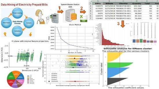
The main aim of this study is to analyze the data of ECPB of Tulkarm district using data mining techniques. A comprehensive data analysis approach is used to analyze ECPB. This approach consists of three key components as shown in Figure 1 and is discussed in detail in Section 3. As a result of this analysis, electricity consumers’ behavior in electricity consumption and their behavior in charging their smart cards are understood and new consumer segmentation is proposed. This will help decision and policy makers at TM to manage the electricity system at strategic, tactical and operational levels.
The structure of this document is presented as follows. Section 2 presents the background of electricity system in Palestine, the state of the art in the field of electricity consumer prepaid bills, and the main novelties of this study. Section 3 presents the key components of the data analysis approach. Section 4 presents the theoretical background of data mining techniques. Section 5 presents the experiment. Section 6 presents the results and discussion. Section 7 presents the conclusion of this study. Finally, abbreviations and references are presented.
2. Background
TM is the main electricity distributor of the Tulkarm district. Tulkarm district, which includes the city and its suburbs and villages is part of the West Bank. TM electricity management system is in an urgent need for improvement. For this reason, it is taken as the sample of this study. This study can be generalized to all West Bank electricity distribution companies, municipalities, and local authorities, because of the similarities of electricity systems setup. The land area of the West Bank including east Jerusalem is 5640 km2, The population as of July 2017 is estimated as of 2,747,943 Palestinians [5]. Tulkarm district’s area is located in the north western part of the West Bank. Its area is about 246 km2 and, as of July 2017, its population is estimated at 166,832 people, representing 12.4% of the population of the West Bank [6]. Tulkarm’s climate is similar to the Mediterranean type, which has long, hot, and dry summers between May and August, and short, cool, and rainy winters between November and March. At the present time, the energy sector in Palestine depends on external energy sources. It heavily dependent on imports from Israel. Palestinian Energy and Natural Resources Authority (PENRA) responsible for developing the energy sector in Palestine. It has implemented several programs to develop the energy sector such as the rehabilitation and expansion of distribution networks and the implementation of rural electrification projects, electrifying more than 98% of the Regulatory Council (PERC) was established in accordance of the Palestinian General Electricity Law. The main responsibility of PERC is to regulate the sector in order to reach a modern and regulated Palestinian electricity sector [7]. As a result of the full dependency of the Israeli electricity supply, six electricity distribution companies and some municipalities and local authorities are responsible of electricity distribution in West Bank and Gaza Strip (WBGS) supervised and controlled by PENRA and PERC. In 1995, since the creation of the Palestinian Authority, the majority of the energy projects have been funded by international aid. The international aid comes from donors, who are seeking to improve the security and stability of the Palestinian energy sector in the WBGS such as, Italy, France, Norway, the Word Bank, and the EU have provided support to reform the regulations and institutions in the sector [2].
TM is currently using a traditional (ordinary) electricity grid that relies on an electronic prepaid metering system using a smart card-operated system. These electronic prepaid meters installed at consumer’s homes and other premises. The consumer purchases credit and then uses the resource until the credit expires. In [8] describes the prepaid metering systems in detail.
TM strategy as mentioned earlier is structured around the reduction of energy consumption through energy conservation and efficiency. One of the key factors to meet this strategy is to understand electricity consumers’ behavior in all sectors. Understanding consumers’ behavior will help the electricity management system to understand how electricity is actually consumed by different consumers and obtain the consumers’ load patterns, electricity consumption’s tariff design, forecasting of scale load, demand response and energy efficiency targeting, detection of loss from non-technical causes, and outliers detection. In addition to the above, it will help in understanding consumers’ behavior in charging their electricity meters’ smart cards in different time periods such as hourly, weekly, daily, etc. This will help electricity management to optimally allocate resources such as opening new vending stations and consumer support centers in peak hours, days, and weekends. To achieve this, a comprehensive data analysis approach is used to analyze ECPB data by using data mining techniques. One of the most important data mining techniques for understanding electricity consumers’ behavior (load profiling) is clustering.
There have been numerous studies to investigate data mining techniques applications in energy consumption such as clustering for electricity consumer segmentation, understanding electricity consumers’ behavior, electricity consumption analysis, data mining based methodologies to support electricity customers’ characterization, etc. For example, in [1] a novel data mining framework is presented and used to explore and extract actionable knowledge from smart meters’ data. Real-time meters’ readings are transmitted to a central location for analysis in order to produce immediate outcomes, in [9] a data-mining-based methodology is presented to support medium voltage electricity customers’ characterization, it relies on smart meter data of 1.022 medium voltage customers, the power consumed was recorded every 15 min in a period of one year, and in [10] a dynamic clustering algorithm is presented and applied. Spanish electricity consumption offline time series data is used for dynamic clustering segmentation of load profiles. The dynamic data represented by feature trajectories in time, etc.
The main novelty of this study in comparison with the previous studies, is that it relies on the analysis and mining of electricity consumers prepaid bills (ECPB) data, which is an offline data with limited features related to the bills of smart card charging by consumers in different time periods. It is about electricity consumers’ smart card charging transactions. The bills’ features are customer (ID, Area, Tariff), bill No., bill date and time, and quantity charged in kWh. Unlike the previous studies that rely on data provided by smart grids, which is an online two-way flow of information at a high frequency, e.g., minutes to hours, which represent the actual consumption of electricity at a specific time period, it might be from 15 min to an hour, day, week, etc. ECPB data is the only source of data available in TM used to know the electricity consumption by consumers and also used for financial accounting issues. This limitations of the data because of the adoption of traditional electricity grid, that relies on traditional prepaid electricity meters. The main aim of this study is to analyze the data of ECPB using data mining techniques. A comprehensive data analysis approach is used to analyze ECPB. As a result of this analysis, electricity consumers’ behavior in electricity consumption and their behavior in charging their smart cards are understood, and new consumer segmentation is proposed. A classification problem is solved, it allows us to predict a certain electricity consumer is belong to which consumer segment. The result and discussion of this study is explained in detail in Section 6. This approach consists of three key components as shown in Figure 1 and is discussed in detail in Section 3. The key components are:
- Data capture, transfer and storage: Electricity data is collected by consumers services centers (Vending Stations), then transferred to System Master Station (SMS), then stored and accumulated in a specific database;
- Data is processed using data analysis, visualization and data mining techniques;
- Management of electricity system will use the result of analysis to support strategic, tactical and operational planning, decision making, and polices drawing of electricity management system at TM.
3. Key Components of the Data Analysis Approach
This approach presents an electricity consumers’ behavior understanding approach supported by knowledge discovery in database (KDD). The main idea is to understand electricity consumers’ behavior in terms of electricity consumption in different time periods, areas, and tariffs (load profiles), and to identify new electricity consumer segmentation by using data mining techniques. To achieve this goal, a methodology is used as shown in Figure 1 consists of three key components and supported by KDD. In [11] KDD is defined as the “nontrivial process of identifying valid, novel, potentially useful, and ultimately understandable patterns or relationships within a data set in order to make important decisions”. In [12] data mining is completely different from straight forward descriptive statistics calculations such as finding the means, standard deviations, or variances. It involves the inference and iteration of many different hypotheses. Pattern generalization from the data sets is one of the key aspects of data mining. Data mining is a well known process with defined steps, each with a set of tasks. The primary objective of data mining is to find the potential useful conclusions that could be acted upon by the users of the analysis. the key components of the ECPB data analysis are:
- Step 1
- Data Capture, Transfer, and Storage.
- Data is captured from different consumer service centers (vending stations) distributed in the Tulkarm district.
- Data is transferred to SMS to ensure a common database.
- Data and feature selection. The first step consists of the data definition, which will be applied to the ECPB data analysis process. Typically, the study of load profiling is implemented based on stored historical data and electricity consumers’ commercial information as well [9]. In this step, the types of consumers selected for the analysis is defined. A good understanding and knowledge of the study application area are required at this phase in order to choose calmly the attributes related to the demand objectives, contracted power, time of day, tariff period, peak power value, geographical areas, etc. The definition of the period of time such as season and year, which is intended to analyze is one of the important tasks, as well as the recorded interval cadence specification [9].
- Electricity consumers prepaid bills data is stored in csv format to form ECPB data set.
- Step 2
- Technology and Algorithm.
- Data pre-processing is applied on the data set to have a cleaned data set ready for analysis.
- Many data pre-processing techniques used in the literature. Section 4 discussed these techniques in detail.
- Data standardization (normalization). See Section 4.1.5.
- Data analysis and data visualization. To obtain a summary and data understanding of the data set, descriptive statistical analysis such as means, standard deviations, medians, variances, correlations, and the five number summary like maximum, minimum, first quartile, third quartile, median and mean are applied. This statistical analysis tells the basic idea how the data set is useful or not for further experimentation. More about statistical analysis is shown in Section 4.2
- Data mining techniques. Data mining is defined in [9] “Is the task of discovering patterns in large data sets involving methods of artificial intelligence, machine learning, statistics, and database systems”. In [10] data mining is considered as an intermediate step with KDD process. This process involves the whole procedure of a data set analysis. The steps are as follows. Data warehousing, which includes all the techniques and procedures to process missing values or errors in data in order to be analyzed. Data mining, which is the intermediate step, the main goal of this step is to extract useful relations or information from the data. The final step is the interpretation of the result, an expert is needed to analyze the obtained results from the data mining procedures in order to draw the conclusions.
- The main techniques applied in the data mining process are as follows. Machine learning, which is classified as Supervised and Unsupervised Learning techniques and algorithms. In supervised learning, we have decision trees, artificial neural networks, Bayes classifier, Association rules, case-base reasoning, genetic algorithm, fuzzy sets, and rough sets. In unsupervised learning, we have clustering, and self-organizing maps. Prediction involves regression models, decision trees, artificial neural network, and support vector machine. Evolution analysis involves time-series data mining, and classification of time-related data.
- Step 3
- Management and Decision MakingFindings and results will support executives, department managers and decision-makers of the electricity system to manage the electricity system in an efficient and effective manner. Electricity systems management is concerning the traditional large consumption customers and also the residential user with medium and high energy consumption, whose electricity consumption depicts abnormal or unbalanced patterns, and peak-off areas where the energy demand remains low [10]. Demand-side management (DSM) tools provide end-user a with valuable interface, information and reports to facilitate energy management. DSM or demand response (DR) as defined by the U.S. Department of Energy technical report: “Changes in electric usage by end-user customers from their normal consumption patterns in response to changes in the price of electricity over time, or to incentive payments designed to induce lower electricity use at times of high wholesale market prices or when system reliability is jeopardized [13]”. Financial incentives and awareness are used to address management by DSM, whereas active management of loads in households and appliances is used by DR [10]. Periodical reports about electricity consumption are sent to electricity consumers by electricity management departments in order to adjust their behaviors to reduce energy costs. This is because of the inability of electricity meters to enable consumers directly review their electricity usage. The awareness of all consumers about energy production and consumption let them adapt their electricity usage during high demand periods, high pricing or lower supply. Therefore, more reliable and stable supply, savings and efficiency will be obtained [14].
4. Theoretical Background of Data Mining Techniques
In this paper, different data mining techniques are used to analyze ECPB. Figure 2 is a data mining work flow that is applied on the data. The literature is full of data mining techniques and their applications in various domains.
The theoretical view of the data mining techniques used in this study are as follows:
4.1. Data Pre-Processing
In general, real-world data or raw data could be incomplete, noisy and/or inconsistent, for instant the incomplete data lacking attribute values. Noisy data contain errors, missing values and/or outliers. Inconsistent data contain discrepancies in codes or names [15]. Major pre-processing techniques used are as follows:
4.1.1. Data Cleaning
The data cleaning process is varying from domain to domain, but basically, it is used to find incomplete, inaccurate, or defect data and then improving the quality of data through correction of detected errors and deletions. The main issue of data cleaning is to find and correct the errors and inconsistencies [16]. Checks for data validation may also include testing for subjugation against applicable standards, conventions, and rules [17].
4.1.2. Data Integration
Data integration is defined in [18] as “The process of obtaining and combining multiple data sources for use in an application”. Multiple databases, data cubes or files are examples of data sources, the destination is a sole or usable format.
4.1.3. Data Transformation
In this phase, data is transformed from one format to another, which is more appropriate for data mining. Data transformation is necessary to facilitate and prepare the data for statistical analysis such as data testing, derived data by computation of the original values, adjusting for outliers by statistical techniques [19]. Smoothing, aggregation, normalization and attribute construction can be applied to the data.
4.1.4. Data Reduction
One of the important issues in data mining now a day is data reduction. Because of the huge size data sets with a maximum which is irrelevant to the objective or some of the data is redundant, dealing with such data as is will increase the consumption of processing power and will generate the wrong results. Here data reduction is a mandatory. Data reduction implies reducing the data but without compromising its integrity [20].
4.1.5. Data Standardization
The central pre-processing step in data mining is Standardization. Standardizing attributes refers to converting values of attributes (features) from one dynamic range into another specific range. Clustering results will be affected depending on the size and variability of the features. Data standardization is an important pre-processing activity to control or scale the variability of the data sets [21]. Improving the accuracy of clustering algorithms and generating good quality clusters are achieved by applying a linear transformation of the raw data (Standardization) to convert the raw data into specific range [21]. Normalization of the data sets features is necessary when measuring Euclidean distance, the outcomes of the clustering are affected by units of measurements of the numerical values of the ranges of dimensional features [22,23]. A universally defined rule for normalization is not exist. Therefore, choosing a normalization rule is left to the discretion of the user [24]. Some of which are (1) natural logarithm; (2) Z-score normalization method; (3) decimal scaling; (4) min–max method; and (5) the Bob–Cox method. Z-score normalization method is taken as an example of applying the normalization process. Let X be an attribute in a data set, the values for an attribute X are standardized based on the mean and standard deviation of X as in Equation (1).
where, and are the mean and standard deviation of x attribute respectively. Generally the Z-score method is useful when the actual minimum and maximum of attribute x are unknown [21]. In this study, a natural logarithm normalization method is used.
4.2. Data Analysis and Data Visualization
Data analysis is defined in [25] as “a process of inspecting, cleansing, transforming, and modeling data with the goal of discovering useful information, informing conclusions, and supporting decision-making. Data analysis has multiple facets and approaches, encompassing diverse techniques under a variety of names, and is used in different business, science, and social science domains. In today’s business world, data analysis plays a role in making decisions more scientific and helping businesses operate more effectively”. Data visualization is defined in [26] as “the science of visual representation of “data”, defined as information which has been abstracted in some schematic form, including attributes or variables for the units of information”. Data are generated in different forms, and used for different purposes. Isolated data has no meaning, but integrated and correlated data within a context, it becomes information with meaning and useful to decision makers [27]. Knowledge is the result of grouping information together. It adds value to the decision-maker for solving problems [28]. Decision maker’s judgment based on prior experiences is required after synthesizing and combining information and prioritizing knowledge [29]. Visionary leader and strategic implementer use data visualization as a popular solution for using big data [30].
4.3. Outliers Detection
An outlier is a datum point, which is unlike the rest of the data set based on some measure. The outlier often refers to abnormal behavior of the system described by data set [31]. Outliers detection is very important in data analysis, the main aim of outliers detection in data mining is to find the dissimilar, inconsistent and exceptional information with respect to the majority of the data set. Outliers detection is applied in many applications in different fields such as financial applications and marketing, fraud detection, network intrusion detection, and network robustness analysis [31]. Breunig in 2000 proposed the local outlier factor (LOF) which is an outlier algorithm used to find irregular data points by using the local deviation of each given data point with respect to its neighbors [32]. The visualization tools can be used to detect outliers, such as box plots and scatter plots. In this paper box plot is used for outliers detection. Box plots are a powerful graphing tool that can be used to improve our understanding of data and allow us to make comparisons across data points [33].
4.4. Clustering
Cluster analysis or clustering is one of the important techniques in data mining [34]. Clustering’s main objective is dividing a data set into some groups, each group called a cluster, such that the more similar data points are located in the same cluster [35]. Clustering is a complex challenge because it entails many methodological choices that determine the quality of a cluster solution [36]. The literature mentioned many different types of clustering algorithms, in [37] a comprehensive classification of clustering algorithms is presented. K-means and single linkage are two types of clustering algorithms use the spectrum analysis of the affinity matrix, which are effective clustering techniques compared with the traditional algorithms [37]. In this paper, the K-keans clustering technique is used because of its simplicity and effectiveness. In clustering, the data sets are assumed to be unlabeled. Clustering as an unsupervised learning problem is frequently considered the most valuable one [38]. It based on the category of centroid-based clustering (partitioning base clustering method). A centroid is a data point at the center of a cluster. In centroid-based clustering, clusters are represented by a central vector. The centroid might not be one of the data set. Centroid-based clustering is an iterative algorithm in which the concept of similarity is derived by how close the distance of a data point is to the centroid of the cluster. In this algorithm, partitioning a data set D of n objects into a set of k clusters, such that the sum of squared distances is minimized. The objective function is as follows in Formula (2).
where, is the distance between a data point and the centroid , which is an indicator of the distance of the n data points from their respective centroids. The significant sensitivity of the initial randomly selected cluster centers is one of the disadvantages of K-means. To reduce this effect, The K-means algorithm can be run multiple times [35].
4.5. Data Classification
Before digging deep into data to find patterns and gain knowledge, you should understand what predictive analysis is. Nyce in [39] defined predictive analysis as the analysis of current and historical facts to make predictions about the future, or otherwise unknown events. This analysis relies on prediction modeling, machine learning and data mining, which are statistical techniques. In predictive analysis, a supervised machine learning algorithm, that is trying to find a variable, which is the target variable according to a labelled data set [40]. One of the important data analysis tasks is classification. Classification is a process of finding a model that distinguishes and describes data classes. It is the problem of finding to which of a set of categories, a new sample belongs to, on the basis of a training set of data containing samples and whose categories membership is known. For example, in this study, we need to classify a new electricity consumer to which groups of consumers (Class) belongs to. A classifier is required to predict class labels such as ‘consumer segment’ for classifying to which group will belong to and to further approve it. The determination of a new electricity consumer to which segment belongs to in advance will help the management function. There are many classification approaches, Kotsiantis in [41] made a detailed review of the most popular Supervised Machine Learning techniques like decision trees, neural networks, naive Bayes, k-nearest neighbor, support vector machine and rule-based machine learning.
5. Experiment
WBGS electricity management systems are in an urgent need for improvement. TM electricity management system is taken as the sample of this study. The method and findings can be generalized to all electricity distributors in WBGS. TM has 18,881 consumers using prepaid electricity meters. Consumers are distributed on 48 different area zones span all Tulkarm district. The consumers are classified according to 27 different types of tariffs such as household, governmental, commercial, industrial, agricultural, etc. A billing processing system captures consumers’ prepayment transaction data. Each transaction, in turn, charges the consumer prepaid smart card. The transactions are recorded in a database. The data from different consumer services centers (vending stations) are consolidated (merged) in CSV Excel file forming ECPB data set. The following are applied on the data sets:
- Data pre-processing techniques, such as data cleaning, integration, transformation, reduction and discretization are applied on the data set.
- Intensive data analysis is implemented on the ECPB data set. Data is analyzed in order to understand consumers’ electricity consumption behavior and consumers’ smart card charging frequencies over time, areas and tariffs. Monthly, weekly, daily, period (evening, morning, and night), and hourly analysis are applied. Electricity consumption summary per area zone and tariff analysis is applied. This analysis is done using descriptive statistics techniques.
- Outliers detection is applied on the data set. Box plot as a visualization tool is used for this purpose.
- K-means clustering algorithm is applied to the ECPB data set. Principal components analysis (PCA) for feature dimensions reduction is applied. One of the main goals of PCA is to reduce the dimensions of the data. Therefore, the complexity of the problem is reduced. Elbow method and silhouette analysis are used to determine the optimal number of clusters to run the K-Means clustering algorithm.
- Classification algorithms are applied. As a result of applying K-Means clustering, new consumer segmentation for electricity consumers is obtained. This new feature is added to the data set and used to apply classification algorithm. Support vector machine (SVM) classifiers are used.
All materials (data sets and codes) are uploaded to github.com. The data sets and codes are shared and can be downloaded freely and used by the public. URL links are provided to the data sets and codes.
The programming environment used in the data analysis is Anaconda 3 (Python 3 distribution) with its popular libraries (Numpy, Scipy, Matplotlib, etc.) [42]. The Data sets and codes files used in this study are uploaded to github.com. It can be downloaded freely to your local drive using this URL link https://github.com/1175maher/Electricity-Data-Mining.
The materials and method used in this study are as follows:
- Step 1
- Install Anaconda 3 and its Python libraries to your computer. You can use the following URL link for the installation. https://www.anaconda.com/distribution/
- Step 2
- Download the data sets and codes files to your local drive. You can use the following URL link to download the data sets and codes files. https://github.com/1175maher/Electricity-Data-Mining. There are 10 files. Three Excel data files (.xlsx), three csv files (.csv) and four Jupyter Notebook Python files (.jpynb). These files are:
- Electricity consumers’ prepaid bills data file. Its name is elect-data.xlsx. It contains all the prepaid bills transactions from June to December 2018. Each row represents one transaction. There are about 250,000 row.
- Consumers’ data file. Its name is clients.xlsx. It contains all electricity consumers’ identification data. There are about 18,000 consumers.
- Tariff data file. Its name is tarif.xlsx. It contains data about consumers’ tariff types such as household, industrial, agricultural, etc. They are about 21 different tariff types.
- Data pre-processing code file. Its name is lelect-data-preprocessing.jpynb. This file contains the code required to clean the raw data file in 1.
- An output file produced after running the code file in 4. Its name is elect-data-phase1.csv.
- Data mapping code file. Its name is elect-mapping-data.jpynb. This file contains the code required to map data files in 2 and 3 with file in 5.
- An output file produced after running the code file in 6. Its name is elect-data-final.csv.
- The data analysis and visualization codes file. Its name is elect-data-analysis-visualization.jpynb. This file contains the codes required for data analysis and visualization using the cleaned and pre-processed data set files in 7, 1 and 2.
- The data mining codes file.Its name is elect-datamining.jpynb. This file contains the codes required for data mining techniques using the data set file in 7.
- The elect-datamining.jpynb is use elect-PCA.csv as an input data file.
- Step 3
- Data pre-processing phase. Open elect-data-perprocessing.jpynb file from the jupyter notebook. Modify the code to setup your data path address. The main input file used here is the elect-data.xlsx file. After running the codes the output file produced is elect-data-phase1.csv file. It is a pre-processed cleaned data set for electricity consumers’ prepaid bills.
- Step 4
- Data mapping phase. Open elect-mapping-data.jpynb file from jupyter notebook. Modify the code to set up your data path address. The main input files used here are the clients.xlsx, tarif.xlsx and elect-data-phase1.csv files. After running the codes the clients and tariffs data are mapped to the electricity consumers’ prepaid bills data in elect-data-phase1.csv file.The output file produced is elect-data-final.csv file. It is a final pre-processed electricity data that is ready for data analysis and mining.
- Step 5
- Data analysis and visualization phase. Open elect-data-analysis-visualization.jpynb file from the jupyter notebook. Modify the code to set up your data path address. The main input files used here are the elect-data-final.csv, clients.xlsx, and tarif.xlsx. After running the codes, data analysis and visualization are implemented and produced.
- Step 6
- Data mining phase. Open elect-datamining.jpynb file from the jupyter notebook. Modify the code to set up your data path address. The main input file used here is the elect-PCA.csv. After running the codes, the data mining techniques such as data normalization, principal components analysis (PCA), elbow method, and silhouette analysis. Clustering and classification are implemented on the data sets.
6. Results and Discussion
TM has 18,881 consumers using prepaid electricity meters. Consumers are distributed on 30 different area zones span all Tulkarm district. The consumers are classified according to 21 different types of tariffs such as household, governmental, commercial, industrial, agricultural, etc. A billing processing system captures consumers prepayment transaction data. Each transaction in turns charges the consumer prepaid smart card. The transactions are recorded in a database. The data from different consumers services centers are consolidated (merged) in CSV Excel file forming ECPB data set. The following phases are applied on the data sets.
6.1. Data Pre-Processing Phase
In this study, data for seven months are collected from the consumer services centers and stored in CSV files covering the period between June and December 2018. Each file contains the following six attributes: bill number, bill date and time, consumer ID, bill quantity charged in Kilo Watt per Hour (kWh), unit price and the total amount of money paid. The collected data are merged in a CSV excel file, and then is mapped with the master consumers and tariff files in order to get the area zone where each consumer belongs to and the tariff type in which each consumer classified (data integration). The file is cleaned from any missing values, not a numeric (NaN) values especially for numerical data (data cleaning). The total amount of money paid attribute is dropped from the data set because it can be derived from the data (data reduction). New attributes are constructed in the data set such as the month-period, month, weekday, weekend, day, period, hour, and peak-hour attributes, which are derived from the date and time attribute. Month-period attribute is 1 if the month attribute value in (June, July, August) or 2 if the month attribute value in (September, October, November), or 3 if the month attribute value in December. Peak-hours attribute is 1 for peak hours if the Hour attribute value between 6 a.m. and 10 a.m. and 5 p.m. and 8 p.m. or 2 for off-peak otherwise. Weekend in Palestine is Saturday and Friday. Friday is a non-working day completely, while Saturday is semi-working day, which means that it is a working day for commercial markets, malls and stores, etc. and a non-working day for governmental institutions, private non-governmental institutions, universities, schools and banks. Therefore, consumers used to charge their prepaid smart card on Thursday (day before the weekend) and on Saturday, these days are the peak week-days or week-end as mentioned in this study. The Week-End attribute value is 1 if the weekday attribute value is (Thursday or Saturday) or 0 otherwise. The period is “evening” if the hour attribute value between 6 p.m. and 8 p.m., “morning” if the hour attribute value between 6 a.m. and 10 a.m., “noon” if the hour attribute value between 11 a.m. and 5 p.m.), “night” otherwise. Some other normalization attributes are added for classification and clustering issues will be discussed later (data transformation). Binning of quantity charged is also applied to classify bills and consumers’ consumption in specific ranges (data discretization). As a result of data pre-processing, a cleaned 250,000 consumers bills csv file is produced. The attributes of the data set and the description is shown in Table 1.
6.2. Data Understanding Phase
The main findings are presented as follows:
6.2.1. Monthly Analysis
Figure 3 shows monthly electricity consumption. The analysis shows that August, July and September having more electricity consumption than other months. August has the most electricity consumption 18.3%, while July and September have 17.7%, 15.9% respectively. Analysis of electricity consumption shows also that the June–August period has more electricity consumption than the September–November period, it is 50.4% over the time period of the data set, while September-November period is 38.6%, while December 11.1%. Consumers tend to use more electricity in the June–August period than the September–November period, this is because of using more electrical appliances. Consumers seeking refuge from the high temperatures, using lights, electronics, and most of all, air conditioning.
6.2.2. Weekly and Daily Analysis
The weekly analysis leads us to see data from a different perspective. The weekly analysis helps management to understand consumers’ behavior in terms of quantities charged per weekdays. Peak week-days are Thursday and Saturday, days before and after weekend, While off-peak weekdays are Sunday, Monday, Tuesday, Wednesday, and Friday. Weekly analysis shows that the total quantity charged in kWh on peak week days (Week-End) is approximately half of the total quantity charged on off peak weak days. Figure 4 shows that 62.2% of the total quantity charged on off peak weekdays, while 37.8% of the total quantity charged on peak weekdays over the time period of the data set.
The weakly analysis helps management to open temporary new service centers in peak weekdays to speed up the charging process and minimize the waiting time of consumers during the charging of smart card process. The daily analysis helps management to understand consumers’ behavior in terms of quantities charged per day. The daily analysis shows that Saturday has the largest total quantity charged 21.4% overall weekdays, followed by Thursday 16.4%, this is a prove that the peak weekdays are Saturday and Thursday. Figure 4 shows the daily distribution of quantity charged over the time period. The analysis shows that Friday which is the main week-end day in Palestine has the smallest quantity charged 4.3% from the overall weekdays.
6.2.3. Period and Hourly Analysis
A day is divided into four time periods as mentioned before. “Evening” period refers to the time period between 6 p.m. and 8 p.m., “morning” refers to the time period between 6 a.m. and 10 a.m., “noon” refers to the time period between 11 a.m. and 5 p.m., and the “night” period otherwise. Period analysis shows that the most quantities charged (50.5%) were in the noon period, followed by a morning period (32%). Figure 5 shows period analysis over the time period of the data set. This analysis will help management understand the consumer behavior in charging their electricity smart cards in terms of time period. The author thinks it is a reasonable result because consumers try to charge their smart cards before going to work or after leaving the work.
TM assumes that peak-hours from 6 a.m. to 10 a.m. and from 5 p.m. to 8 p.m. and off peak-hours otherwise. Figure 5 shows that the total electricity charged on peak-hours is 55.7%, while 44.3% of electricity charged is off peak-hours.
6.2.4. Electricity Consumption Summary per Area Zone
Analysis shows that the consumers behavior in electricity consumption and in charging their prepaid smart cards are varied depends on time periods. The most electricity consumed and quantities charged is in area 10 (North), followed by area 1 (South), and then area 47 (Tulkarm) and so on in all timing periods, this is due to area population size differences. This can be seen in Figure 6.
6.2.5. Tariff Analysis
TM classified consumers according to 27 different tariffs such as household, governmental, commercial, industrial, agricultural, etc. They do not account for any other factors in the classification of consumers. Prices per kWh vary according to consumers’ tariff type. The following is the tariff analysis of the existing system. In the next clustering section, K-means clustering algorithm is applied on the data set to create a new consumer segmentation taking into account other factors. Figure 7 shows the electricity consumption for each tariff type over the time period of the data set. Household is the most electricity consumption 69.8% overall other tariffs type, followed by governmental tariff type 23.3%, then municipality employee tariff type 6.9%. Tariff analysis shows that some consumers move from tariff to another for example tariff Temp1 has no transactions in October, November and December, this implies that consumers of this tariff type transferred to another tariff after September.
6.2.6. Feature Transformation by Using Principal Component Analysis (PCA)
The main aim of using PCA is to reduce the dimensionality of large data sets, but at the same time minimize information loss [43]. In this study, PCA is used to obtain a two-dimension (2D) visualization of all electricity consumers. It allows us to compare consumers at a glance according to ECPB data set’s four features. PCA is applied on the pre-processed data set to find the dimensions about the data that maximize the variance of features involved. The explained variance ratio of each dimension will also be reported as well. A PCA component or dimension can be considered a new “feature” of the space. This feature is a composition of the original features present in the data. Figure 8 shows that the first and second features, in total, explain approximately 83.4% of the variance in the data set. The first three features, in total, explain approximately 95.3% of the variance. In terms of electricity consumers,
- Dimension 1 has a high negative weight for AreaNo feature and low negative weight for Quantity feature. This dimension might represent electricity consumers located in areas with high Areano and consume low quantities.
- Dimension 2 has a high negative weight for Quantity feature, and medium positive weight for BillNo feature, and low positive weight for AreaNo feature. This dimension might represent electricity consumers who consume large quantities per month and charge their smart card a moderate number of times per month and located in areas with low Areano.
- Dimension 3 has a high positive weight for BillNo feature, and medium positive weight for Quantity feature, and approximately 0 weight for AreaNo feature, and low negative weight for TariffNo feature. This dimension might represent electricity consumers who charge their smart card large number of times per month, consumes medium quantites, located in one specific AreaNo, and have Tariff Type with low TariffNo.
As mentioned before, one of the main goals of PCA implementation is to reduce the dimensions of the data. Therefore, the complexity of the problem is reduced. In this study, PCA is used to obtain a two-dimension (2D) visualization of all electricity consumers. Figure 9 shows a biplot (scatterplot), where X-axis represents the first principal component or dimension and the Y-axis represents the second component or dimension. Each data point is represented by its scores along the principal components. The biplot shows the projection of the original features along the components. It helps us understand the reduced dimensions of the data, and find relationships between the principal components and original features. As seen in the Figure 9 the original feature projections (in blue) and it is easy to understand the relative position of each data point in the scatterplot. For example, a point the lower left corner of the figure will likely correspond to a consumer that consumes a high quantity per month and belongs to a high AreaNo. We can observe that Quantity as well as AreaNo at the two most important components.
6.3. Outliers Detection
Figure 10 shows a box plot, that illustrating a large number of outliers. After analyzing some of these outliers the following result is achieved:
- The most electricity consumption per month by ConsumerID Y00010828-001105, which belongs to AreaNo 10 (North) and TariffID 5 (Governmental), is a government institution. This is a justifiable consumption.
- Some large quantities of electricity consumption per month by many consumers such as ConsumerID Y00005543-001476 who belong to AreaNo 47 (Tulkarm) and TariffNo 6 (Commercial), it is a commercial economic entity. This is a justifiable consumption.
- Some large quantities of electricity consumption per month by many consumers who belong to TariffNo 3 (Household). This is not justifiable and more investigation should be conducted on them. Table 2 shows a list of consumers who have large quantities of electricity consumption per month.
6.4. Clustering (The Application of K-Means Clustering on The Data Set)
The electricity system management in TM, as mentioned in the tariff analysis section, used to classify electricity consumers according to their tariffs. The main objective of this classification is the pricing of the kWh for each consumer tariff. This classification method does not take into account any other features such as quantities consumed per month and areas where consumers are located. At present TM electricity management is planning to classify electricity consumers according to the total quantities consumed in kWh per month and areas in which consumers are located. As a result of applying K-Means clustering on the data set four clusters are obtained. This will enhance electricity consumer segmentation in order to better understand consumers’ behavior and extract more knowledge about electricity consumption issues such as demand, pricing, exemptions, discounts, and others. K-means clustering is used for this purpose and discussed in detail in the next section.
Clustering as an unsupervised data mining technique is implemented on ECPB data set to propose a new consumer segmentation. Electricity consumer segmentation is the sub division of an electricity consumer base into groups called consumer segments such that each consumer segment consists of consumers who share similar electricity consumption characteristics. This segmentation is based on factors that can directly or indirectly influence electricity consumption such as consumer area, tariffs, average quantities charged per month and average number of times consumers charging their smart card per month (average number of bills per month). The importance of consumer segmentation includes, inter alia, the ability of TM to well manage the electricity demand that will be suitable for each of its consumer segments. In this paper, the K-means clustering algorithm has been applied in consumer segmentation. K-means algorithm provided by Sklearn Python Library is applied.
6.4.1. Clustering for Consumers Segmentation
The proposed methodology comprises data pre-processing, data analysis and visualization, abnormal consumption detection, clustering and classification of consumers. It enables understanding electricity consumers’ behavior and segmenting electricity consumers. ECPB data set contains data about electricity consumers. Each record represents an electricity consumer such as ConsumerID, Quantity, BillNo, AreaNo and TariffNo. Where Quantity is the average quantity of electricity consumed per month, BillNo is the average number of times consumer’s electricity smart card is charged per month, Areano is the area where the consumer is located in Tulkarm district and TariffNo is the tariff type the consumer belongs to such as household, agricultural, manufacturer, governmental, etc. For the purpose of targeting a specific type of electricity consumers with similar behavior and characteristics. Machine learning can be used to accomplish this task. Particularly, clustering, it is an unsupervised learning problem, that has the ability to find categories, grouping similar consumers. These categories are called clusters. A collection of points in a data set refers to a cluster, the more similarities of these points let them belong to the same cluster, while the dissimilar points are belonging to other clusters. Distance-based clustering groups the points into some number of clusters such that small distances within the cluster, while large distances between clusters.
The application of K-Means based on the following assumptions:
- The shape of cluster: clusters shape is spherical, which means the distribution variance is spherical. We have to have a normally distributed variables with the same variance.
- The size of cluster: the same number of observations for all clusters.
- The correlation between variables: no or little correlation between the variables.
The variables of the data set are tested by applying the required descriptive statistics on ECPB data set before normalization. Therefore, the variables of the data set are not normally distributed and variances are not close to each other. Logarithm transformation on data set, which is a simpler approach and works in most cases, is applied to the data set to correct non-normal distributed variables or non-equal variances. The result of logarithm scaling is seen in Figure 11, the distribution of each feature is more normal and there is no correlation between the variables. In order to be a way from skew of K-means clustering results, outliers detection is a mandatory for the data.
6.4.2. Deciding the Optimal Number of Clusters Using Elbow Method
The number of clusters must be decided in advance when we want to apply the K-Means clustering. The elbow method is used to decide the optimal numbers of clusters. This method uses the concept of minimizing within-cluster sum of square (WCSS). A scree plot is created which plots the number of clusters in the x-axis and the WCSS for each cluster number in the y-axis. Figure 12, as the number of clusters increase, the WCSS keeps decreasing. The decrease of WCSS is initially steep and then the rate of decrease slows down resulting in an elbow plot. The elbow formation in the graph gives an indication of the number of clusters, in addition to the knowledge of the case are used to decide the optimal number of clusters. The elbow may not be cleared, it may indicate that there may not be any natural groups in the data [44] or may have more than one elbow in the graph, it may indicate that more than one natural group of clusters fit the data [45]. The elbow method presents the variation of the number of clusters with the total WCSS. For that, K-Means is computed with different values of k (number of clusters). Then, the total WCSS is calculated and WCSS vs. number of clusters curve is plotted. Then, the elbow is located in the plot. The minimization of the WCSS is the main objective. This point is considered to be the optimal number of clusters.
6.4.3. Deciding the Optimal Number of Clusters Using Silhouette Analysis
Silhouette analysis is used as a validation of the measurement WCSS along with the elbow method to find the optimal number of clusters for the K-Means algorithm application. The separation distance between clusters can be analyzed using silhouette analysis. The measure of how close every point in a cluster is pointed in the neighboring clusters is displayed by the silhouette plot. This can be used to evaluate parameters like the number of clusters visually. This measure has a range from −1 to 1, it is called the silhouette coefficients. If the silhouette coefficient near +1, that means the sample is far away from neighboring clusters. A value of 0 means that the sample on or very close to the boundary between neighboring clusters and negative values indicate that those samples might have been assigned to the wrong cluster. As a result of using WCSS along with the elbow method, the number of clusters k = 4 is chosen as seen in Figure 12. Figure 13, Figure 14, Figure 15, Figure 16 and Figure 17 show silhouette plots. The easier way to determine the optimal number of clusters using this method is to group together graphs when n-cluster= 3, 5, and 6, this gives the graph with n-cluster = 4, and also group together graphs when n-clusters = 2 and 4 gives also the graph with n-clusters = 4. Therefore, the optimal number of clusters = 4. Therefore, the optimal number of clusters in both methods (elbow and silhouette) are four clusters.
6.4.4. Applying K-means Clustering with Number of Cluster Is Four (k = 4)
Four clusters or consumer segments are identified. The four features considered in the clustering are the normalized average quantity charged of electricity in kWh by consumers per month, the normalized average number of bills charged by consumers per month, the normalized area number and the normalized tariff number that are consumer belongs to. The most important features appear to be the Average Quantity Consumed per month in kWh and AreaNo in which electricity consumers belong to. As a result of WCSS minimization along with elbow method and Silhouette Analysis, the optimal number of clusters used in K-Means clustering is four. Figure 18 shows K-Means plots of the clusters according to the mentioned data set features. Four consumer clusters or segments are identified and labeled thus:
- Cluster 0: consumers with quantities between (20 and 1000) kWh and distributed in areas where AreaNo between (14 and 48).
- Cluster 1: consumers with quantities less than 4000 kWh and are located in AreaNo 1.
- Cluster 2: consumers with quantities between (20 and 7500) kWh and distributed in areas where AreaNo between (4 and 47).
- Cluster 3: consumers with quantities less than or equal 400 kWh and distributed in areas where AreaNo between (4 and 29).
Setting the number of clusters to four might provide a meaningful consumer segmentation. This will help the managers of TM in their strategic, tactical and operational planning as follows:
- The ability of the management to draw their policies and set their programs that will be suitable for each of its consumer-segment.
- Predicting the electricity consumption associated with each segment and effectively and efficiently manage the forces of demand and supply.
- Unravelling some latent dependencies amongst consumers such that their behavior in electricity consumption, number of times they charge their smart cards per month, etc.
- Management and decision support in terms of risky situations such as shortages in electricity supply in case of electricity cut off.
- Forecasting the growth in demand for electricity for each consumer segment.
- Forecasting of the growth rates in new consumers in the coming months.
- Understanding consumers’ distributions in each area and the number of times each consumer segments charging their smart cards per month to make decisions to open new vending stations and to know the feasibility of their opening.
The main question arises now, how we can evaluate the K-means clustering algorithm? In general, it is really hard to figure out if our clustering is good or not. Evaluating cluster is not a well developed or is usually used as a part of cluster analysis. It might be because of its very nature. Even so, the evaluation and validation of clustering is important. As a result of the number of different type of clusters, in other words, each clustering algorithm defines its own type of clusters. It may seem that each clustering might entail a different evaluation measure. Some are using an extrinsic approach for clustering evaluation, which means that using clustering results to solve another problem or task. For example, identifying and eliminating outliers. Another example train different classifiers for each sub-population. Others use an intrinsic approach for clustering evaluation. that means using clustering results to understand the makeup of data, that would be a qualitative type of evaluation.
6.5. Classification
The main classification problem is the identification of a set of categories or sub-populations belongs to which group (cluster) on the basis of a training set of data, that contains observations and whose categories membership is known. For example, suppose we have to predict whether a given electricity consumer belongs to consumer segment (class) 0, 1, 2, or 3, after training a set of ECPB data. To solve this problem applying the classification technique is a mandatory. In this case, a classifier is used to predict class labels such as consumer segment ‘0, 1, 2 or 3’ for classifying electricity consumers.
As a result of K-means clustering, a new attribute is added to the data set named consumer-segment. This labeled data set will be used in a classification model. Now the data set contains (ConsumerID, normalized average quantity per month, normalized average number of bills per month, normalized area, Normalized tariffNo, and consumer-segment). ECPB with the consumer-segment feature is a labeled data set. K-Means is used to find clusters within the data set and test how good it is as a feature. The data set then is divided into train and test data sets. SVM classifier is applied on the data set. The consumer-segment attribute values are 0, 1, 2, or 3 this refer to cluster 0, cluster 1, cluster 2, or 0 cluster 3 respectively. This class attribute is used to determine the consumer segment that a consumer belongs to. The following classification task is applied. Suppose we have to predict whether a given electricity consumer belongs to consumer segments 0, 1, 2, or 3, on the basis of four variables, the average electricity quantity consumed per month, the average number of prepaid bills per month, the area and tariff the consumer belongs to. These variables are called features. To solve this classification problem, a set of ECPB observations called training data set, which is prepared from the actual electricity prepaid bills and the classification results come from the K-means clustering algorithm. A model is trained and used to predict whether a certain consumer will belong to consumer segments 0, 1, 2, or 3. Therefore, the outcome depends upon the ability of features to map to the outcome. Evaluation of the quality of the model by statistical and mathematical measures to check to what extent the classifier generalizes the relationship between the features and the outcome using the optimal parameter values obtained on the training data sets, the accuracy was examined using independent test data sets. The classification accuracy is the ratio of correct prediction to total prediction made. As a result of the SVM classification method application on data sets, the classification accuracy is 93.4%. It can be observed that SVM has a significance performance measure. Therefore, the machine learning classifier based on SVM algorithm applied on the consumer electricity prepaid bills’ data set is more than 93% accurate in predicting whether a consumer belongs to consumer segment 0, 1, 2, or 3.
The accuracy of classification alone is not enough, because it can be misguiding, particularly if we have an unequal number of observations in each class or as in our case if we have more than two classes. Confusion matrix calculation is the solution. The confusion matrix summarizes the performance of the classification algorithm and gives us better information about how our classification model is improvinf and also what types of errors are making. Therefore, the confusion matrix is a mandatory in our work because it can be used to see more detail about the performance of the model. It is a summary of prediction results on a classification problem. The next section is a detail discussion of classification performance.
6.5.1. Classification Performance Results
SVM classification method is applied by using the the scikit-learn for machine learning in Python. ECPB data set is divided into the training data set and test data set. The test data set is 35% of the data set. The result of applying the SVM classifier is shown in Table 3 confusion matrix.
6.5.2. Discussion of Confusion Matrix
The results of the classification model is shown in Table 3. It shows the confusion matrix after applying the SVM classifier. It is a summary of prediction results. The problem is to predict whether a certain electricity consumer will belong to consumer segment (class) 0, 1, 2, or 3. It is a four-class confusion matrix. This matrix helps us to understand the type of errors that occur during the testing and training data sets. The confusion matrix, cm is a 4 × 4 matrix. Its rows and columns refer to the ground truth and predicted class labels of the data set, respectively. In other words, each element, , refers to the number of observations of class i that were assigned to class j by the SVM classification method. For instance, the number of observations of class 1 that were assigned to class 0 by SVM classifier is 104. The diagonal of the confusion matrix gives the correct classification decisions (i = j). Count values in the matrix show the number of correct and incorrect predictions, and broken down by each class. The ways in which the classification model is confused when it makes predictions is shown. Insight not only into errors, but type of errors being made by classifier are given. It is an excellent choice for reporting results in 4-class classification problems because the relations between the classifier outputs and the true ones is possible to be observed. In 2-class confusion matrix, identification of the four possible results, true positive (TP), false positive (FP), false negative (FN), and true negative (TN), that means correctly classified or predicted, incorrectly classified or predicted (type I error), incorrectly rejected (type II error), and correctly rejected, respectively is easy. In a four-class confusion matrix, where the elements in the confusion matrix, where i is row identifier and j is column identifier, refer to the cases belonging to i that had been classified as j. The total numbers of true positive (TTP), false positive (TFP), false negative (TFN), and true negative (TTN) for each class i (i = 0, 1, 2, 3) will be calculated as:
In our case 1351 + 867 + 1940 + 1871 = 6029 times. That means that the total number of times over the samples were correctly classified or predicted is 6029 times.
In our case 32 + 0 + 11 = 44 times. That means we have 44 times non-class 2 classified or predicted as class 2.
In our case 0 + 0 + 0 = 0 times. That means all class 1 instances that are not classified or predicted as class 1 are 0 times.
In our case 1351 + 32 + 26 + 94 + 1940 + 9 + 153 + 11 + 1871 = 5487 times. That means all non-class 1 instances that are not classified or predicted as class 1 are 5487 times.
In our case the total number of cases is 6458 cases. To evaluate the overall accuracy of the classifier:
In our case the overall accuracy of SVM classifier is 93.3%, obviously, the 1—overall accuracy is the overall classification error, which is 6.7%.
The measure of the overall accuracy is characterizes the classifier as whole. There are three class-specific measures, that describe how well the SVM classifier algorithm performs on each class. Firstly, the class recall measures, R(i), which is the proportion of data with true class label i that were correctly assigned to class i. In other words, out of all positive classes, how much we predicted correctly? It should be high as possible.
In our case the recall measure of class 0, which correctly assigned class 0 is 0.99 (99%). Secondly, the class precision, P(i), which is the fraction of observations that are correctly classified to class i if we take into account the total number of observations that are classified to that class. In other words, out of all positive classes we have predicted correctly, how many are actually positive.
In our case the precision measure of class 2, which measures the fraction of data, which are correctly classified to class 2 if we take into account the total number of data, which are classified to class 2 is 0.993 (99.3%). Thirdly, the class specificity measures, S(i), which answer the question that out of all negative classes we have predicted correctly, how many are actually negative?
Finally, we conclude that SVM classifier can be used to predict whether a certain electricity consumer will belong to the consumer segment (class) 0, 1, 2, or 3 with a high degree of accuracy.
7. Conclusions
In this study, a comprehensive data analysis approach supported by KDD is used. Different data mining techniques for understanding electricity consumers’ behavior are applied to the ECPB data set. Data pre-processing, outliers detection, and normalization are applied. A common method to cluster the ECPB data set into groups with similar characteristics was chosen. K-Means clustering algorithm is used to achieve this objective. Principal components analysis (PCA) for feature transformation is used. The main goal of using PCA is to reduce the dimensions of the data and to obtain a two-dimension (2D) visualization of all electricity consumers. It allows us to compare consumers at a glance according to ECPB data set’s four features. The appropriate number of clusters is verified through the use of elbow and silhouette methods. The ECPB data set is a successful group together in a cluster, in which each cluster consisted of electricity consumers with similar consumption behavior. Classification algorithms are used based on the consumer segmentation feature of K-Means clustering results to enable the classification of new consumers. The classification algorithms present a good overall accuracy.
As a result we conclude the following:
- Outliers detection. A list of household electricity consumers with huge electricity consumption per month is created in order to do more consumer investigation.
- A new consumer segmentation is proposed by implementing the K-Means clustering algorithm, four consumer clusters or segments are identified and labeled. The advantages of the new consumers segmentation compared with the existing segmentation, that the existing segmentation relies on the consumers’ tariff only (household, agricultural, governmental, manufacturer, etc.), while the new proposed consumers segmentation help electricity management system to understand how electricity is actually consumed for different consumers and obtain the consumers’ load profiles or load patterns, tariff design related to the electricity consumption, consumer scale load forecasting, demand response and energy efficiency targeting, non-technical loss detection and outliers detection. Moreover, the management can benefit from This new consumers segmentation as follows:
- (a)
- Drawing policies and programs that will be suitable for each of its consumer-segment.
- (b)
- Predicting the electricity consumption for each segment and effectively and efficiently manage the forces of demand and supply.
- (c)
- Unravelling some latent dependencies amongst consumers such that their behavior in electricity consumption, number of times they charge their smart cards per month etc.
- (d)
- Managing risky situations such as shortages in electricity supply in case of electricity cut off.
- (e)
- Forecasting the growth in demand of electricity for each consumer segments.
- (f)
- Forecasting of the growth rates in new consumers in the coming months.
- (g)
- Evaluating the feasibility of opening new vending stations for each consumer segment to better serving them.
- A new consumer segmentation feature is added to the data set and then a classification problem is solved by SVM classification method. Confusion matrices are produced to show the accuracy of the classification and prediction.
Funding
This research received no external funding.
Acknowledgments
It is my pleasure to thank the senior management of Tulkarm municipality particularly, the mayor, the Information Technology and electricity management departments for their support in providing me the raw data of the consumers electricity prepaid bills of Tulkarm district.
Conflicts of Interest
The author declare no conflict of interest.
Abbreviations
The following abbreviations are used in this manuscript:
| TM | TulKarm Municipality |
| ECPB | Electricity consumers prepaid bills |
| PENRA | Palestinian Energy and Natural Resources Authority |
| PERC | Palestinian Electricity Regulatory Council |
| WBGS | West Bank and Gaza Strip |
| SMS | System master station |
| KDD | Knowledge discovery in database |
| DSM | Demand side management |
| DR | Demand response |
| kWh | Kilo Watt per Hour |
| PCA | Principal components analysis |
| WCSS | Within cluster sum of square |
| SVM | Support vector machine |
References
- Silva, D.; Xinghuo, Y.; Alahakoon, D.; Holmes, G. Data Mining Framework for Electricity Consumption Analysis From Meter Data. IEEE Trans. Ind. Inform. 2011, 7, 399–407. [Google Scholar] [CrossRef]
- CES-MED. Municipality of Tulkarm Sustainable Energy Action Plan (SEAP). 4 January 2016. Available online: https://www.ces-med.eu/sites/default/files/SEAP_Tulkarem_Palestine.pdf (accessed on 14 April 2019).
- Wang, Y.; Chen, Q.; Kang, C.; Xia, Q. Clustering of electricity consumption behavior dynamics toward Big Data applications. IEEE Trans. Smart Grid 2016, 7. [Google Scholar] [CrossRef]
- Granell, R.; Axon, C.; Wallom, D. Impacts of raw data temporal resolution using selected clustering methods on residential electricity load profiles. IEEE Trans. Power Syst. 2015, 30, 3217–3224. [Google Scholar] [CrossRef]
- The World Factbook-Middle East: West Bank. Central Intelligence Agency, 26 September 2018. Available online: https://www.cia.gov/library/publications/the-world-factbook/geos/we.html (accessed on 3 October 2018).
- PCBS (Palestinian Central Bureau of Statistics). Demographic Survey of the West Bank and Gaza Strip; District Report Series. No. 1–9; PCBS: Ramallah, Palestine, 2010.
- Palestinian Electricity Regulatory Council (PERC). Annual Report; PERC: Ramallah, Palestine, 2011. [Google Scholar]
- Bandyopadhyay, K. User acceptance of prepayment metering systems in India. Int. J. Indian Cult. Bus. Manag. 2008, 1, 450–465. [Google Scholar] [CrossRef]
- Ramos, S.; Duarte, J.; Vale, Z. A Data-mining based Methodology to support MV Electricity Customers’ Characterization. Energy Build. 2015. [Google Scholar] [CrossRef]
- Benitez, I.; Quijano, A.; Diez, J.; Delgado, I. Dynamic clustering segmentation applied to load profiles for energy consumption from Spanish customers. Electr. Power Energy Syst. 2014, 437–448. [Google Scholar] [CrossRef]
- Fayyad, U.; Piatetsky-shapiro, G.; Smyth, P. From data science to knowledge discovery in databases. AI Mag. 1996, 17, 37–45. [Google Scholar]
- Vijay, K.; Bala, D. Predictive Analytics and Data Mining Concepts and Practice with Rapidminer; Morgan Kaufmann: Burlington, MA, USA, 2015. [Google Scholar]
- Benefits of Demand Response in Electricity Markets and Recommendations for Achieving Them; Tech. Rep.; U.S. Department of Energy: New York, NY, USA, 2005.
- Alahakoon, D.; Yu, X. Smart electricity meter data intelligence for future energy systems: A survey. IEEE Trans. Ind. Inform. 2015. [Google Scholar] [CrossRef]
- Bhatt, C. Data Visualization and Visual Data Mining. CSI Communications. January 2014. Available online: https://www.researchgate.net/publication/259922079-Data-Visualization-and-Visual-Data-Mining (accessed on 4 April 2019).
- Kumar, K.; Chadrasekaran, R.M. Attribute Correction-Data Cleaning Using Association Rule and Clustering Methods. Int. J. Data Min. Knowl. Manag. Process 2011, 1. [Google Scholar] [CrossRef]
- Chapman, D. Principles and Methods of Data Cleaning: Primary Species and Species-Occurrence Data; Version 1.0.; Global Biodiversity Information Facility: Copenhagen, Denmark, 2005; Available online: http://www.gbif.org/document/80528 (accessed on 3 April 2019).
- Bazeer, A.; Ramkumar, T. Data Integration-Challenges, Techniques and Future Directions: A Comprehensive Study. Indian J. Sci. Technol. 2016, 9. [Google Scholar] [CrossRef]
- Manikandan, S. Preparing to analyze data. J. Pharmacol. Pharmacother. 2010, 1, 64–65. [Google Scholar] [CrossRef]
- Vora, P.; Oza, B. Improved Data Reduction Technique in Data Mining. IJCSMC 2013, 2, 169–174. [Google Scholar]
- Bin Mohamad, I.; Usman, D. Standardization and Its Effects on K-Means Clustering Algorithm. Res. J. Appl. Sci. Eng. Technol. 2013, 6, 3299–3303. [Google Scholar] [CrossRef]
- Aksoy, S.; Haralick, R. Feature normalization and likelihood-based similarity measures for image retrieval. Pattern Recognit. Lett. 2001, 22, 563–582. [Google Scholar] [CrossRef]
- Larose, D. Discovering Knowledge in Data: An Introduction to Data Mining; Wiley: Hoboken, NJ, USA, 2005. [Google Scholar]
- Karthikeyani, N.; Thangavel, K. Impact of Normalization in Distributed K-Means Clustering. Int. J. Soft Comput. 2009, 4, 168–172. [Google Scholar]
- Xia, B.; Gong, P. Review of business intelligence through data analysis. Benchmark. Int. J. 2014, 21, 300–311. [Google Scholar] [CrossRef]
- Friendly, M.; Denis, D.; Truman, S. Milestones in the History of Thematic Cartography, Statistical Graphics, and Data Visualization. Project. History of Data Visualization January 2001. Available online: https://www.researchgate.net/project/History-of-Data-Visualization (accessed on 13 April 2019).
- Świgoń, M. Information limits: Definition, typology and types. Aslib Proc. 2011, 63, 364–379. [Google Scholar] [CrossRef]
- Mandinach, E.; Honey, M.; Light, D. A theoretical framework for data-driven decision making. In Proceedings of the Annual Meeting of the American Educational Research Association, San Francisco, CA, USA, 1–5 April 2006. [Google Scholar]
- Siemens, G. Connectivism: A learning theory for the digital age. Int. J. Instruct. Technol. Distance Learn. 2005, 2, 3–10. [Google Scholar]
- Moore, J. Data visualization in support of executive decision making. Interdiscip. J. Inf. Knowl. Manag. 2017, 12, 125–138. [Google Scholar] [CrossRef]
- Aggarwal, C.; Yu, P. An effective and efficient algorithm for high-dimensional outlier detection. VLDB J. 2005, 14, 211–221. [Google Scholar] [CrossRef]
- Breunig, M.; Kriegel, H.; Ng, R.; Sander, J. Lof: Identifying density-based local outliers. In Proceedings of the 2000 ACM SIGMOD International Conference on Management of Data, Dallas, TX, USA, 15–18 May 2000; Volume 29, pp. 93–104. [Google Scholar]
- Krzywinski, M.; Altman, N. Visualizing samples with box plots. Nat. Method 2014, 11, 119–120. [Google Scholar] [CrossRef]
- Zhao, Q.; Franti, P. Centroid Ratio for a Pairwise Random Swap Clustering Algorithm. IEEE Trans. Knowl. Data Eng. 2014, 26. [Google Scholar] [CrossRef]
- Badase, S.; Deshbhratar, G.; Bhagat, A. Classification and Analysis of Clustering Algorithms for Large Datasets. In Proceedings of the International Conference on Innovations in Information, Embedded and Communication Systems (ICIIECS), Coimbatore, India, 19–20 March 2015. [Google Scholar] [CrossRef]
- Ketchen, D.; Shook, C. The Application of Cluster Analysis in Strategic Management Research: An Analysis and Critique. Strateg. Manag. J. 1996, 17, 441–458. [Google Scholar] [CrossRef]
- Niu, D.; Dy, J.; Jordan, M. Iterative Discovery of Multiple Alternative Clustering Views. IEEE Trans. Pattern Anal. Mach. Intell. 2014, 36, 1340–1353. [Google Scholar] [CrossRef]
- Cios, K.; Pedrycz, W.; Swiniarski, R.; Kurgan, L. Data Mining: A Knowledge Discovery Approach; Springer: New York, NY, USA, 2007. [Google Scholar]
- Nyce, C. Predictive Analytics White Paper. In American Institute for CPCU; Insurance Institute of America: Malvern, PA, USA, 2007; pp. 9–10. Available online: https://www.the-digital-insurer.com/wp-content/uploads/2013/12/78-Predictive-Modeling-White-Paper.pdf (accessed on 18 September 2019).
- Gmyzin, D. A Comparison of Supervised Machine Learning Classification Techniques and Theory-Driven Approaches for the Prediction of Subjective Mental Workload. Master’s Thesis, Dublin Institute of Technology, Dublin, Ireland, 2017. [Google Scholar] [CrossRef]
- Kotsiantis, S. Supervised machine learning: A review of classification techniques. Informatica 2007, 31, 249–268. [Google Scholar]
- Ryan Spain, G. Python and R in Big Data and Data Science. 2018 DZone Guide to Big Data: Stream Processing, Statistics, and Scalability. Available online: https://dzone.com/articles/dzone-research-5 (accessed on 4 April 2019).
- Jolliffe, I.; Cadima, J. Principal component analysis: A review and recent developments. Philos. Trans. A Math. Phys. Eng Sci. 2016, 374, 20150202. [Google Scholar] [CrossRef]
- Hambrick, D.; Schecter, S. Turnaround strategies for mature industrial-product business units. Acad. Manag. J. 1983, 26, 231–248. [Google Scholar] [CrossRef]
- Aldenderfer, M.; Blashfield, R. Cluster Analysis; Sage: Newbury Park, CA, USA, 1984. [Google Scholar] [CrossRef]
Figure 1.
Key components of data analysis approach.

Figure 2.
Data mining work flow applied in the study.

Figure 3.
Monthly consumption in kWh.

Figure 4.
Electricity quantity charged in kWh weekly and daily.

Figure 5.
Electricity quantity charged in kWh per hour.

Figure 6.
Average consumption in kWh per month per area.

Figure 7.
Electricity consumed in kWh per tariff.

Figure 8.
PCA dimensions.

Figure 9.
PC plane with original feature projections.

Figure 10.
Outliers detection of electricity consumption in kWh per month.

Figure 11.
ECPB data set variables distribution and correlation.

Figure 12.
Elbow method for finding the optimal number of clusters.

Figure 13.
Silhouette analysis where the number of clusters is 2.

Figure 14.
Silhouette analysis where the number of clusters is 3.

Figure 15.
Silhouette analysis where the number of clusters is 4.

Figure 16.
Silhouette analysis where the number of clusters is 5.

Figure 17.
Silhouette analysis where the number of clusters is 6.

Figure 18.
K-means clustering plot.


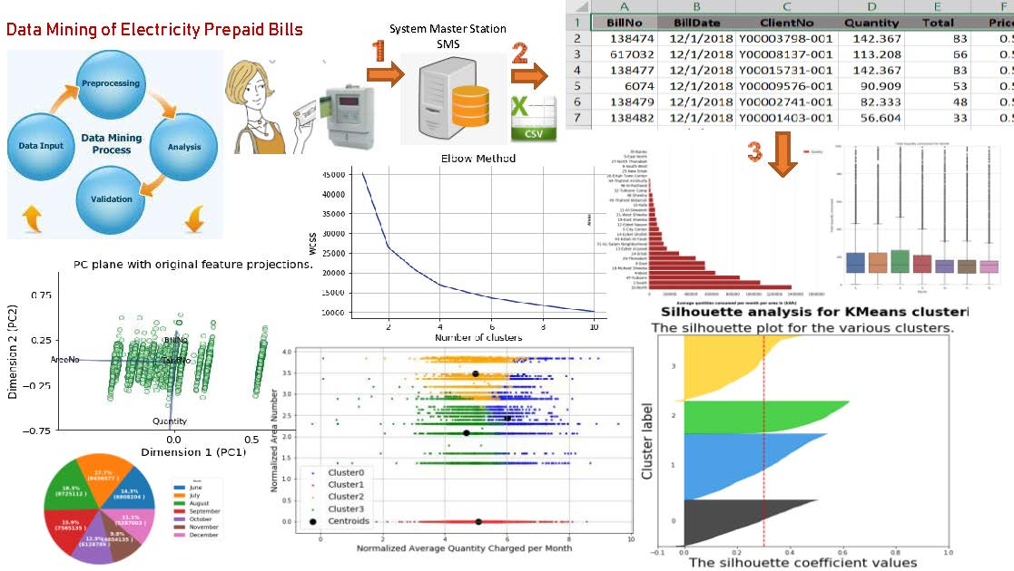
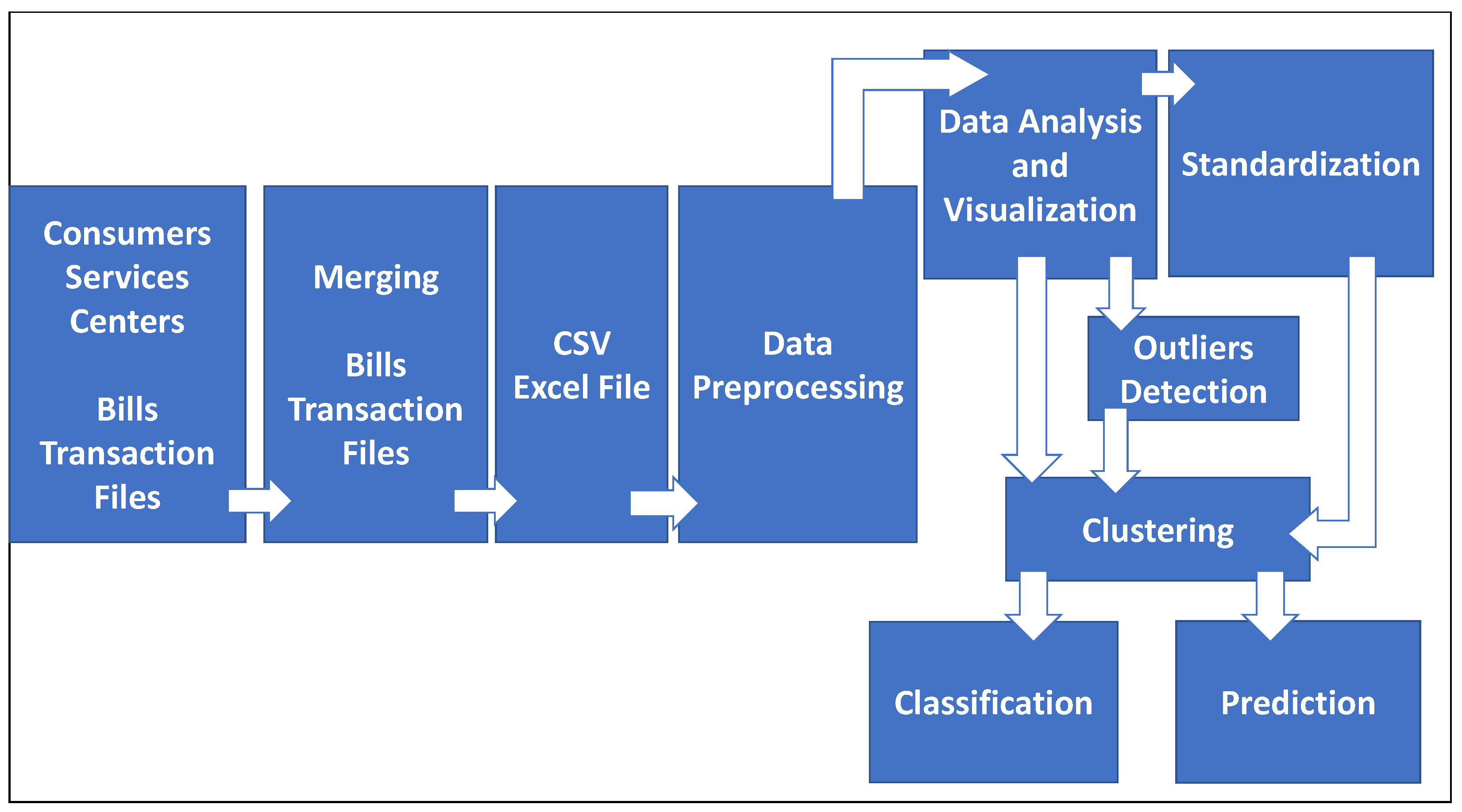
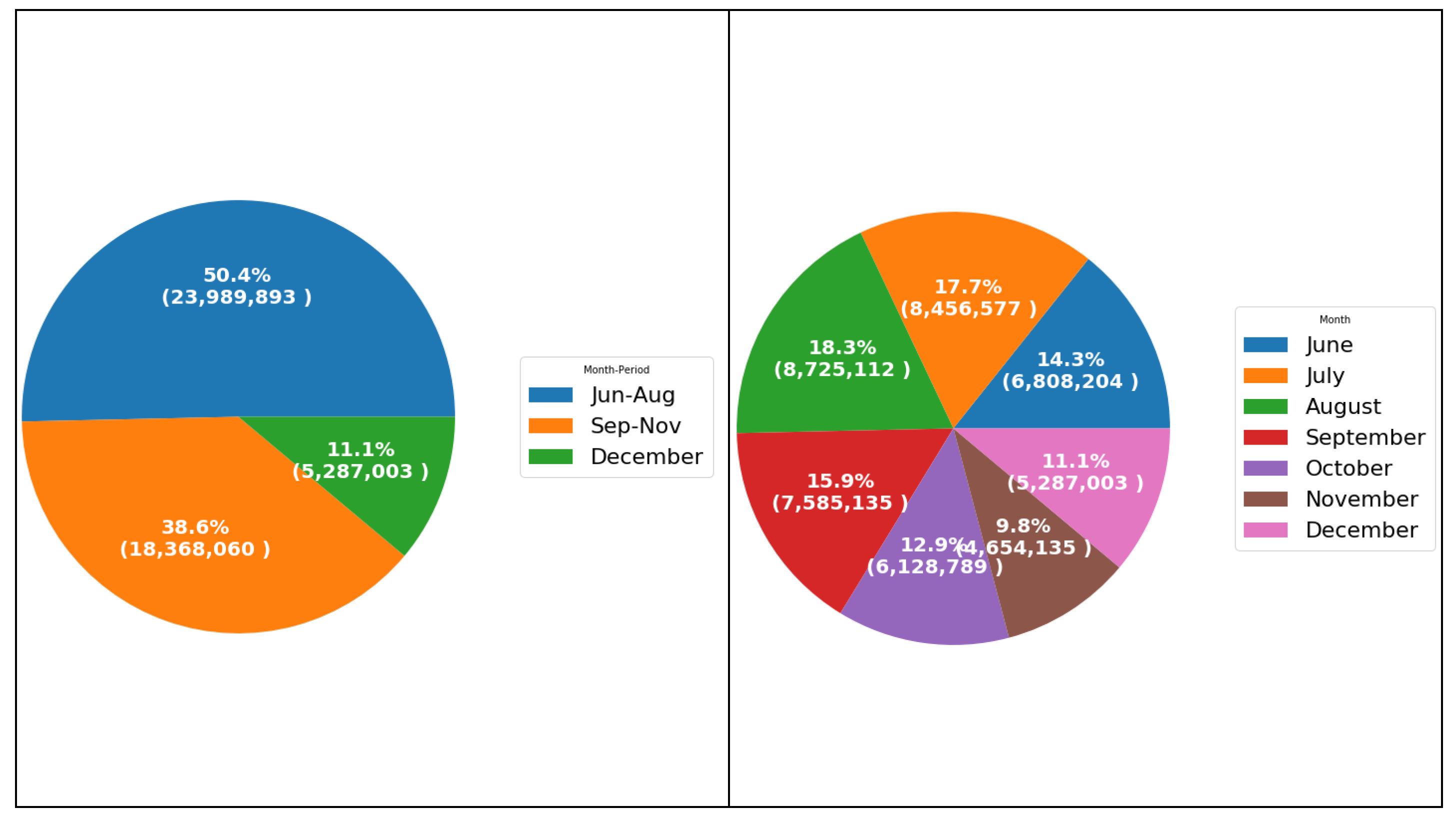
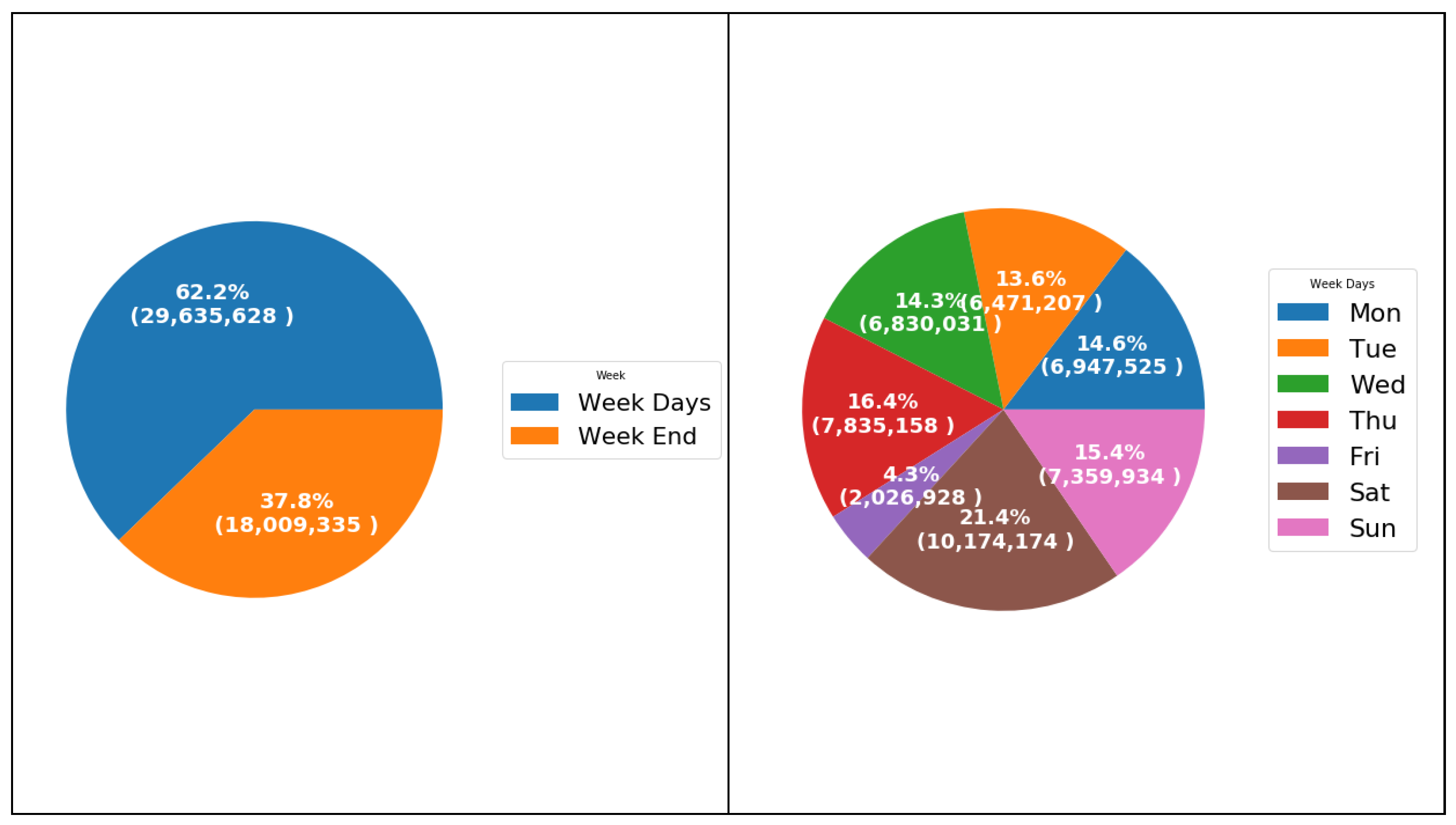
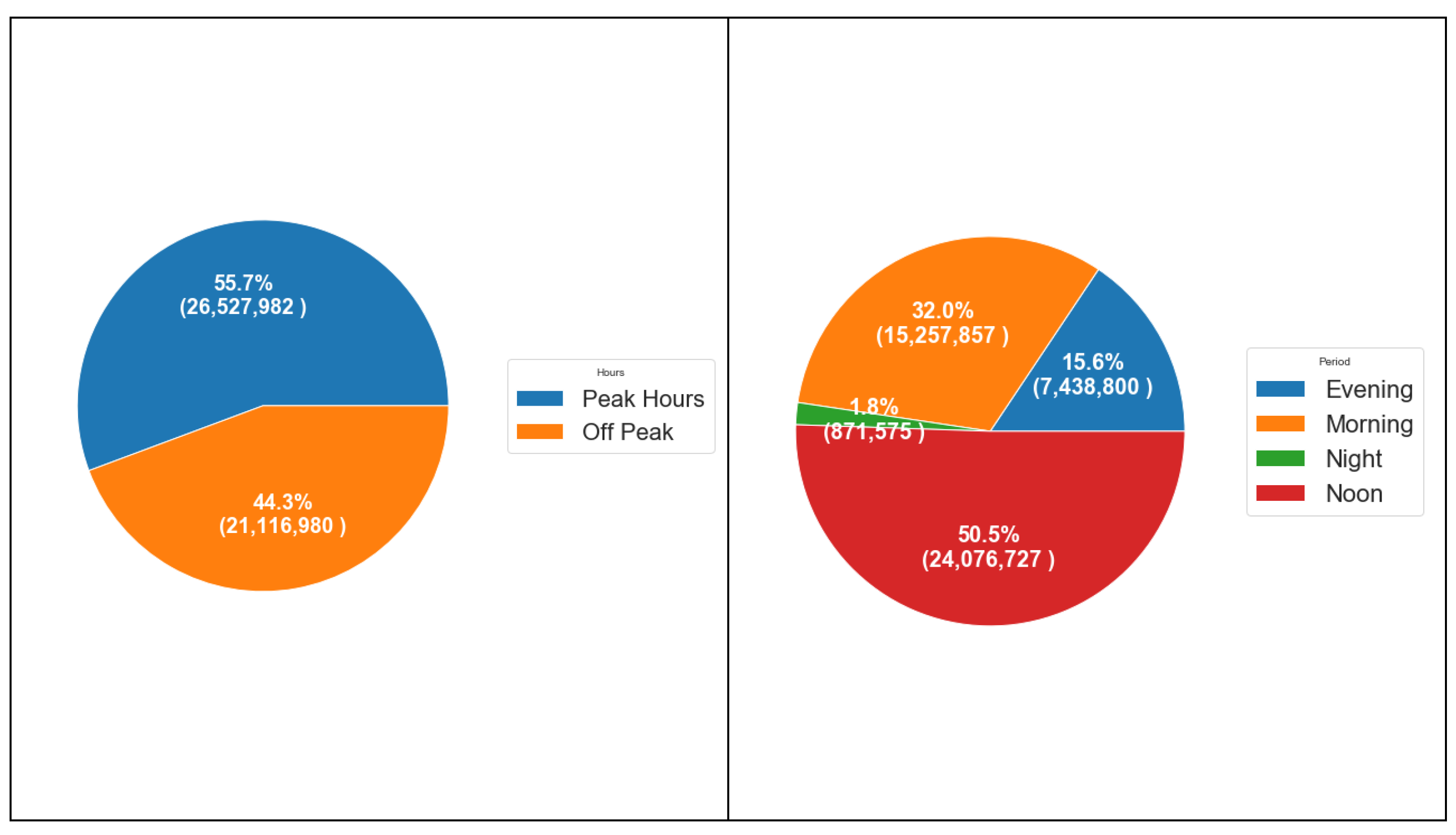
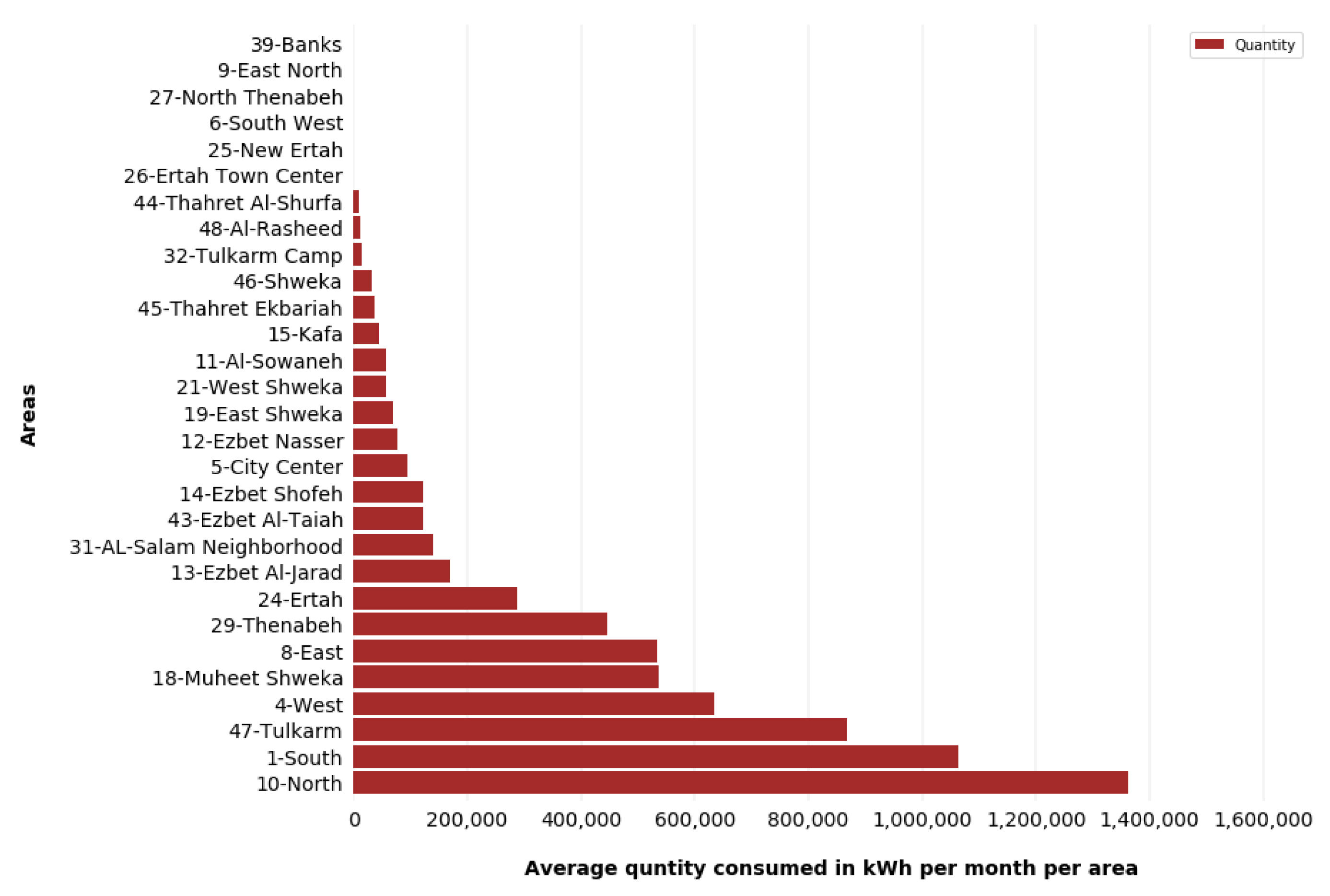
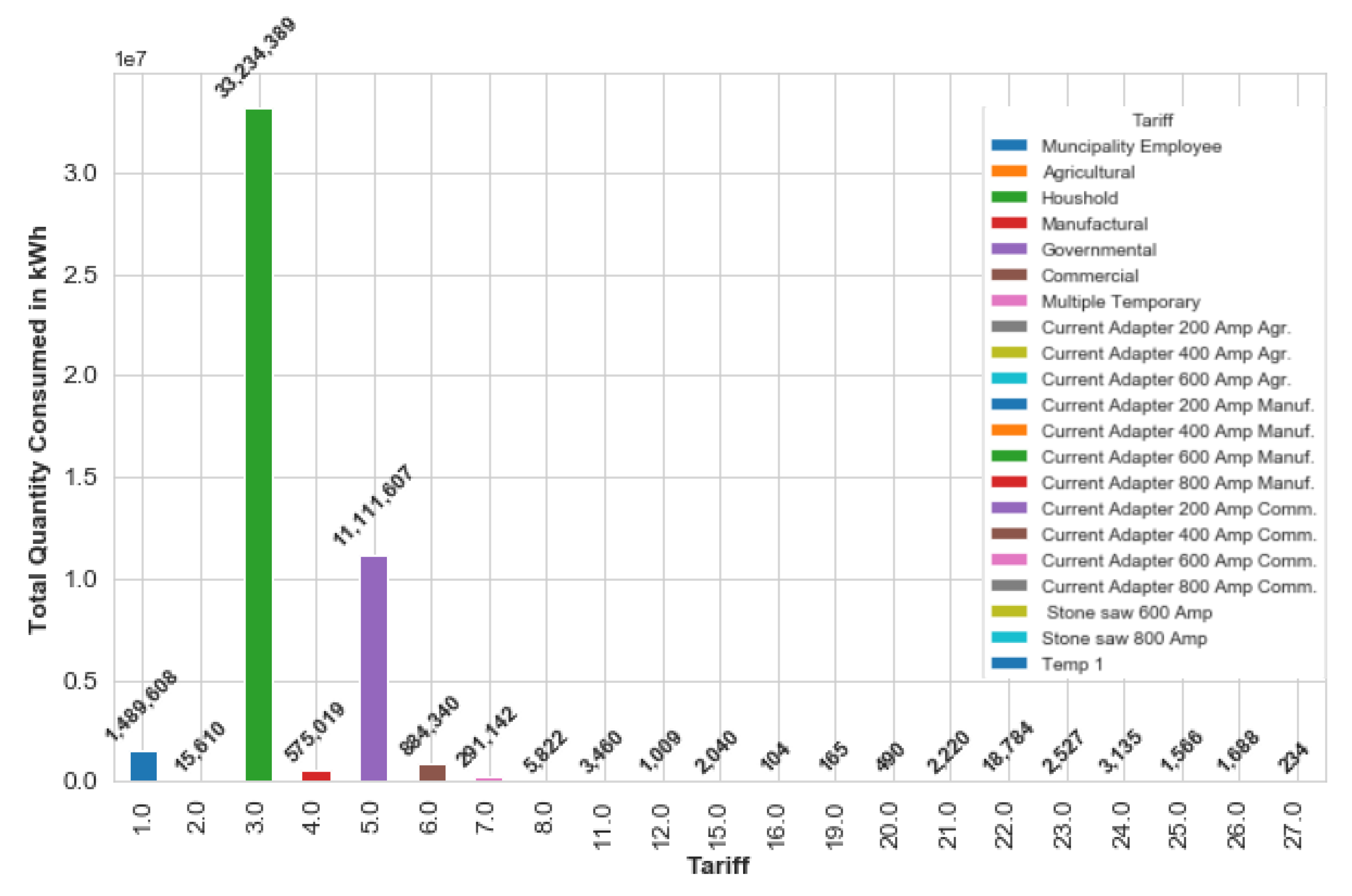
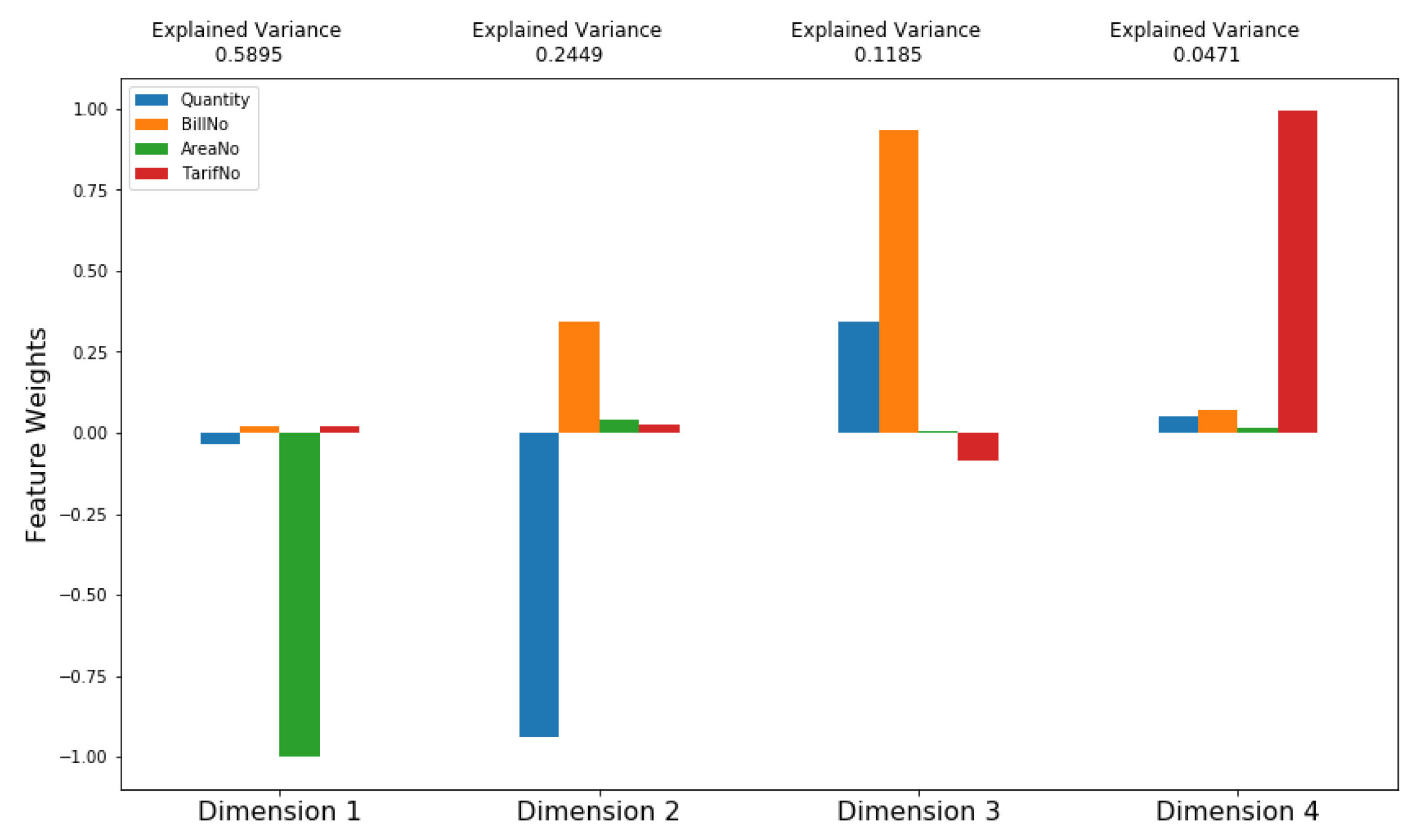
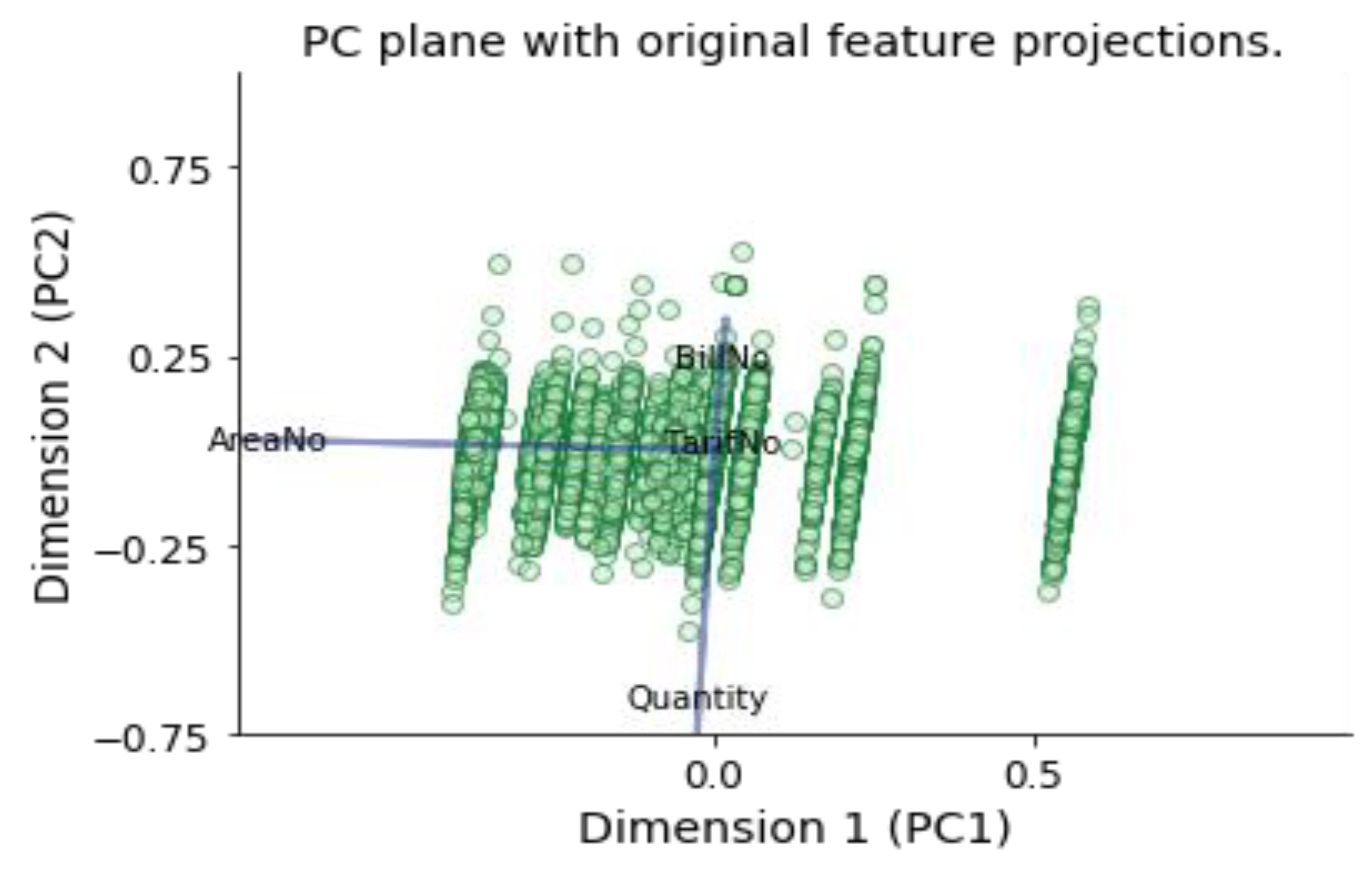
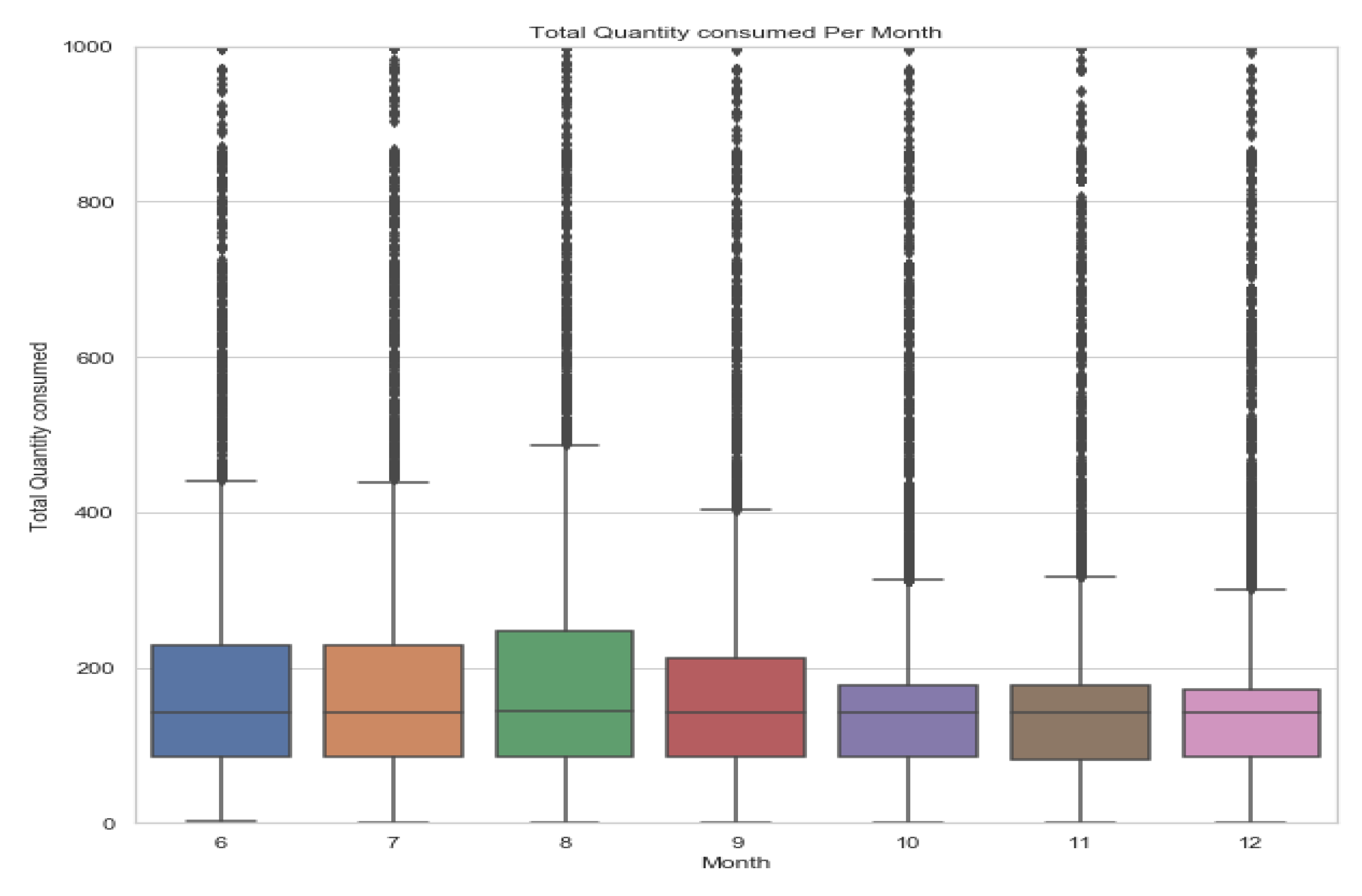
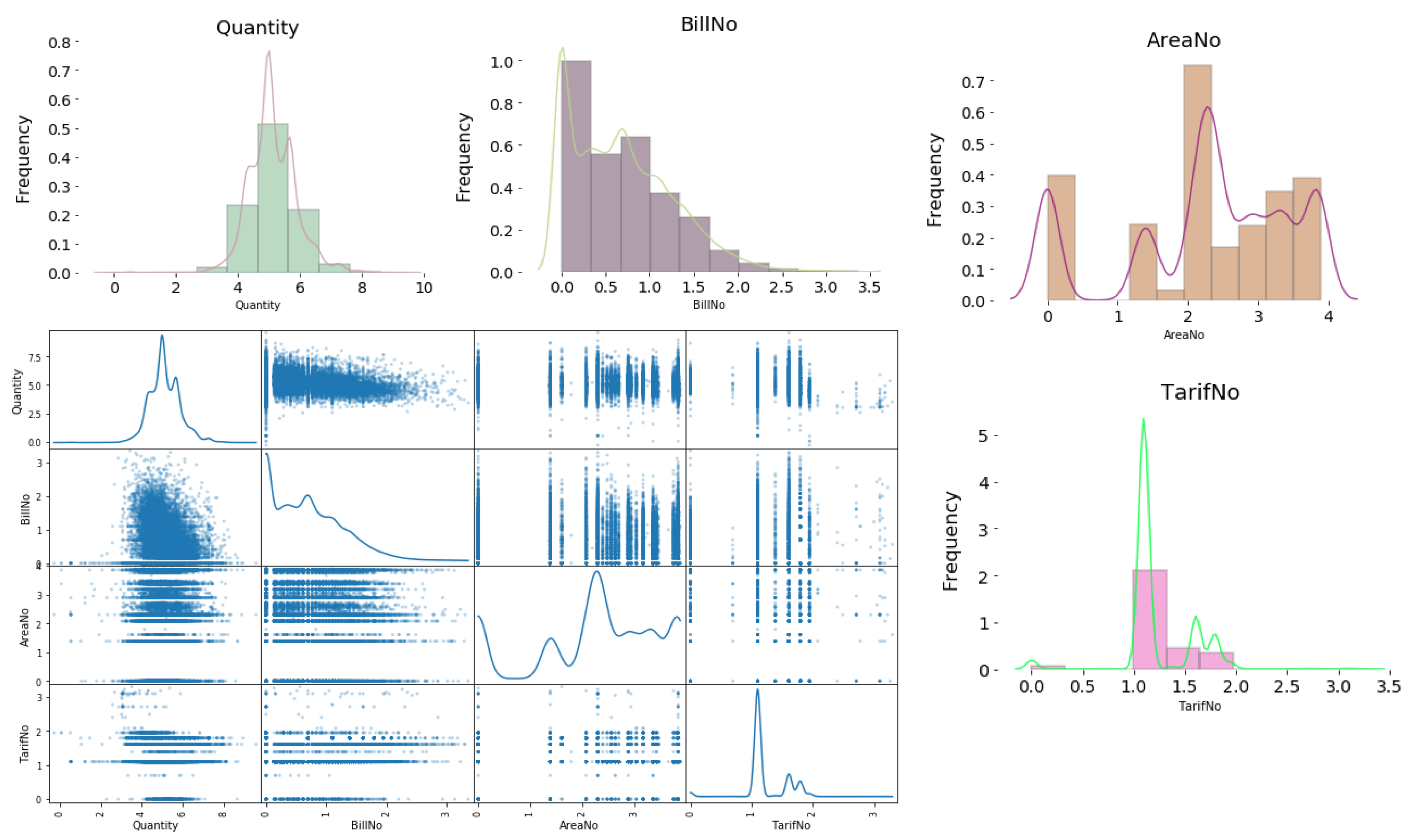
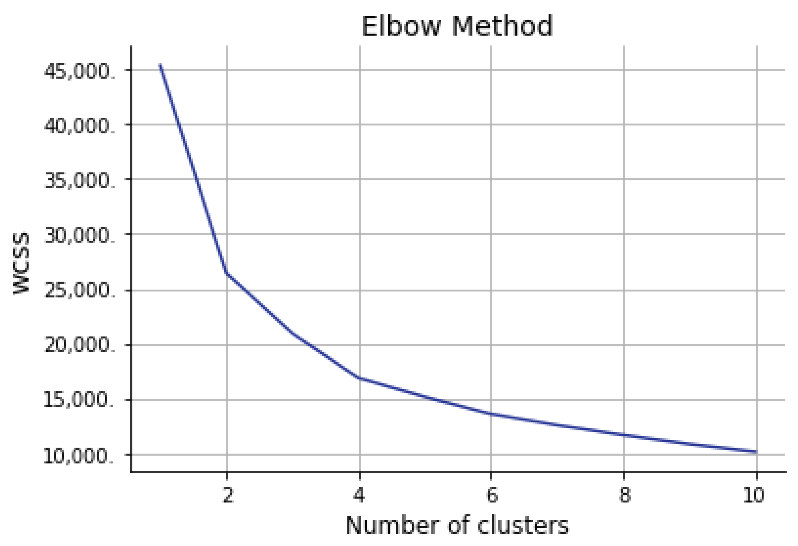
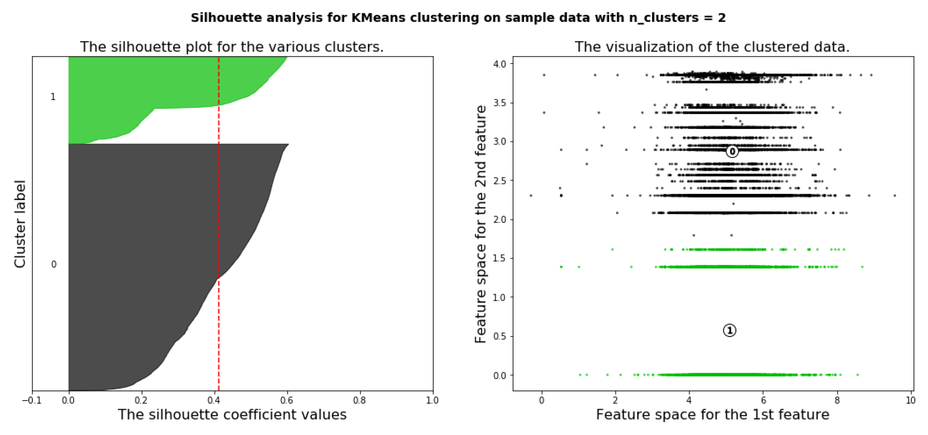
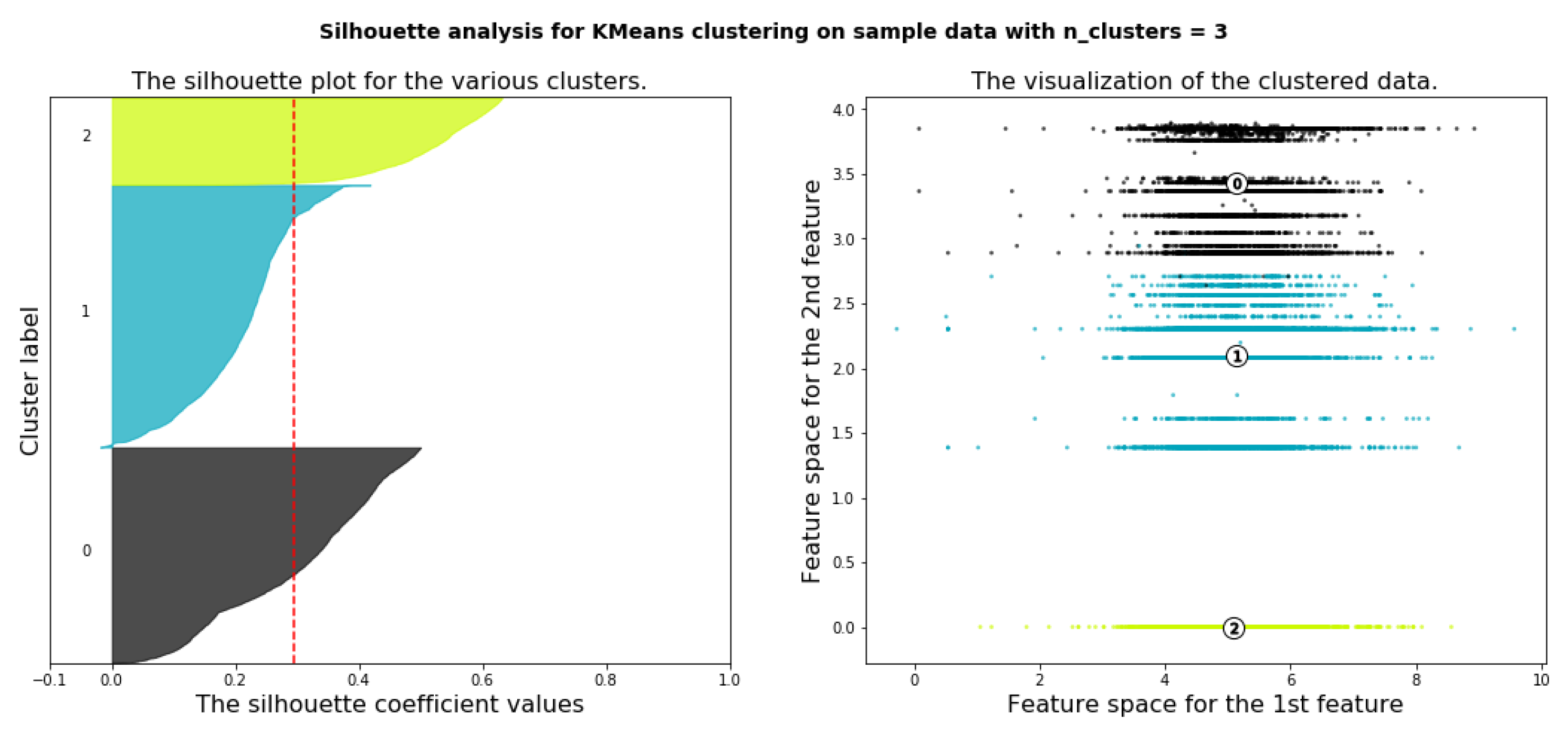
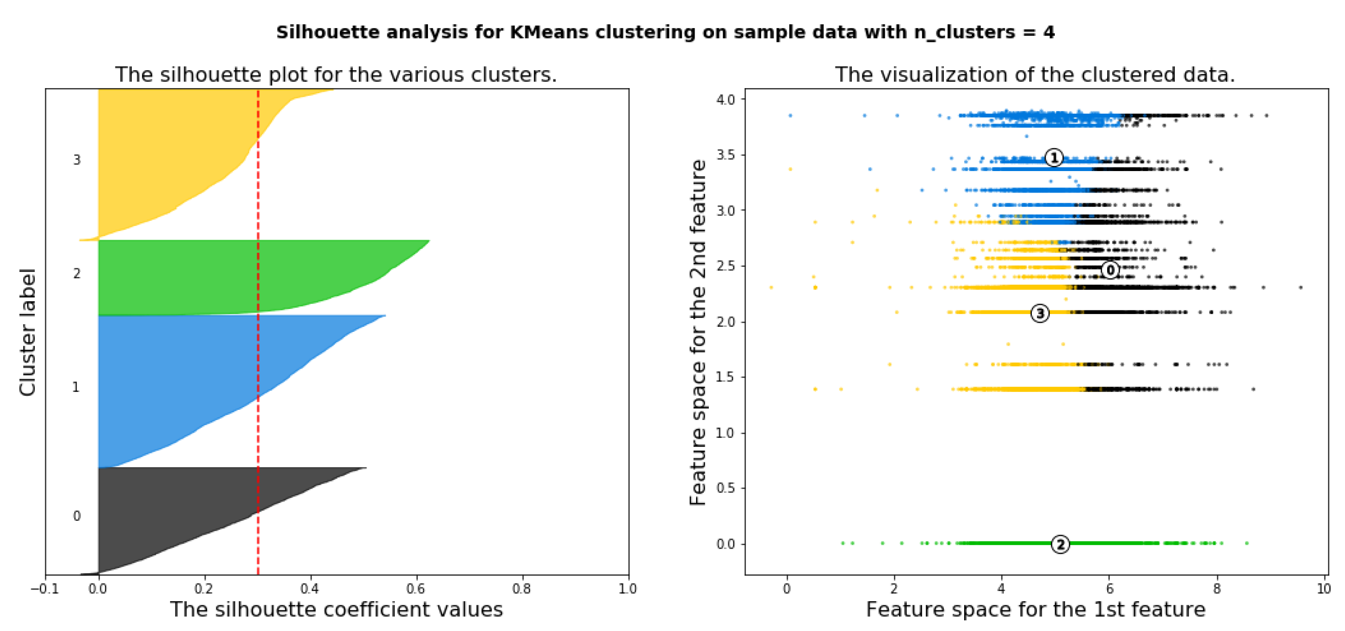
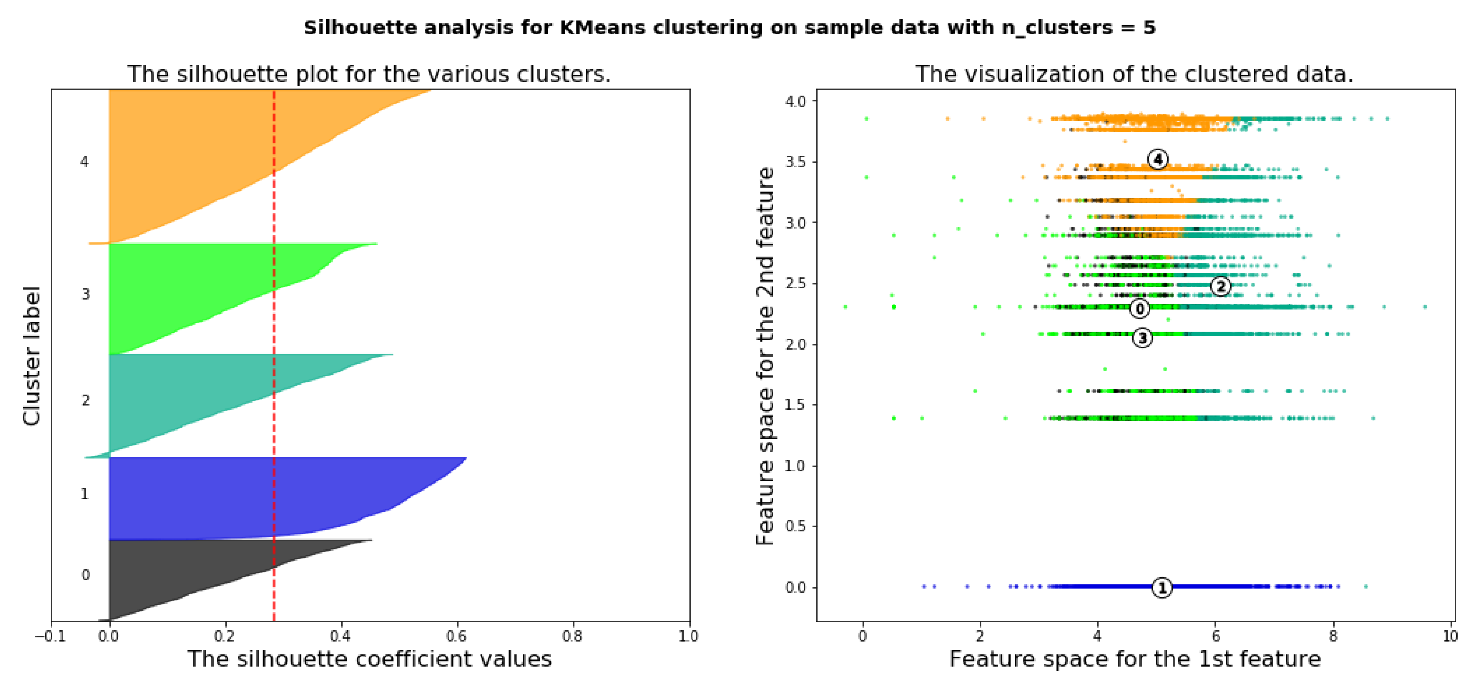
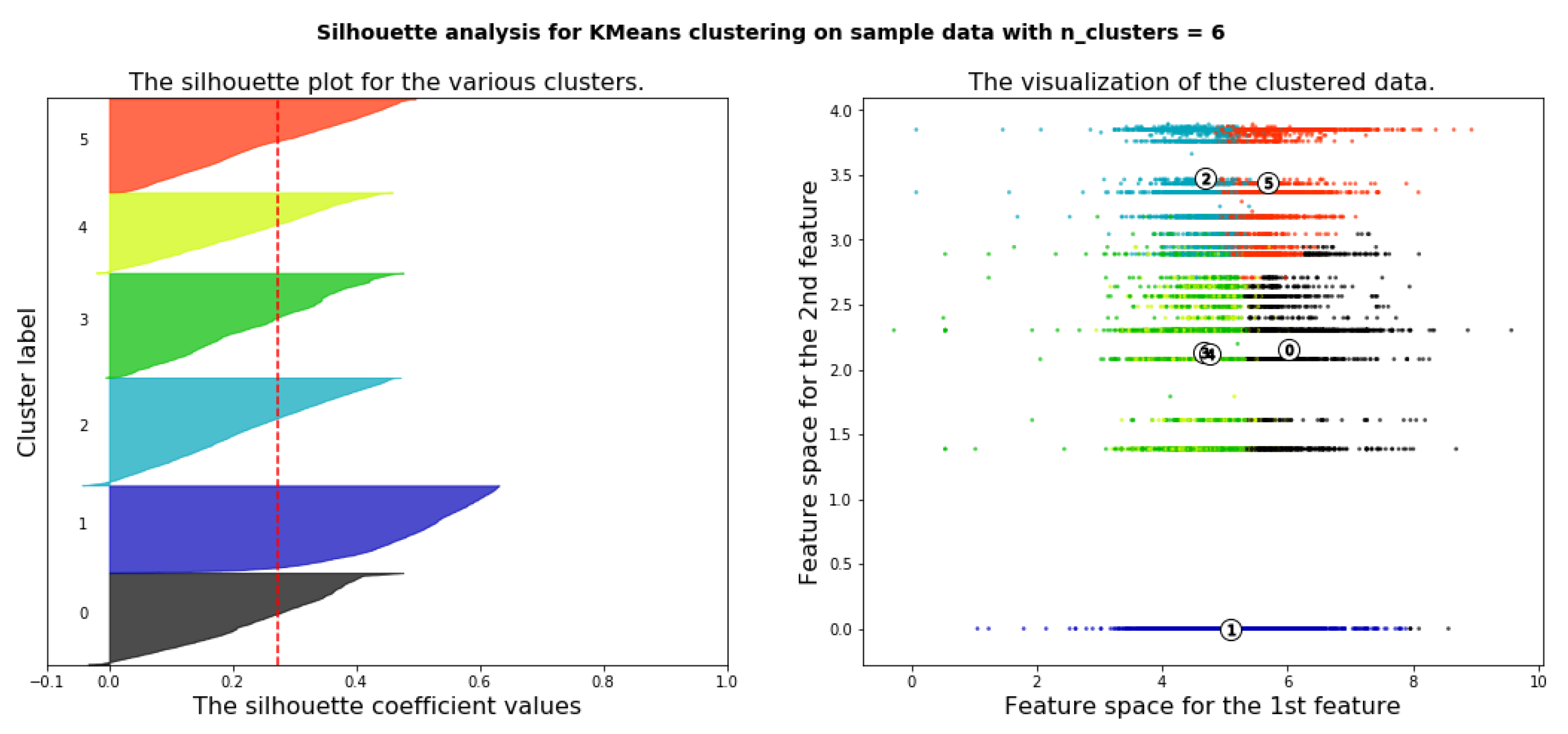
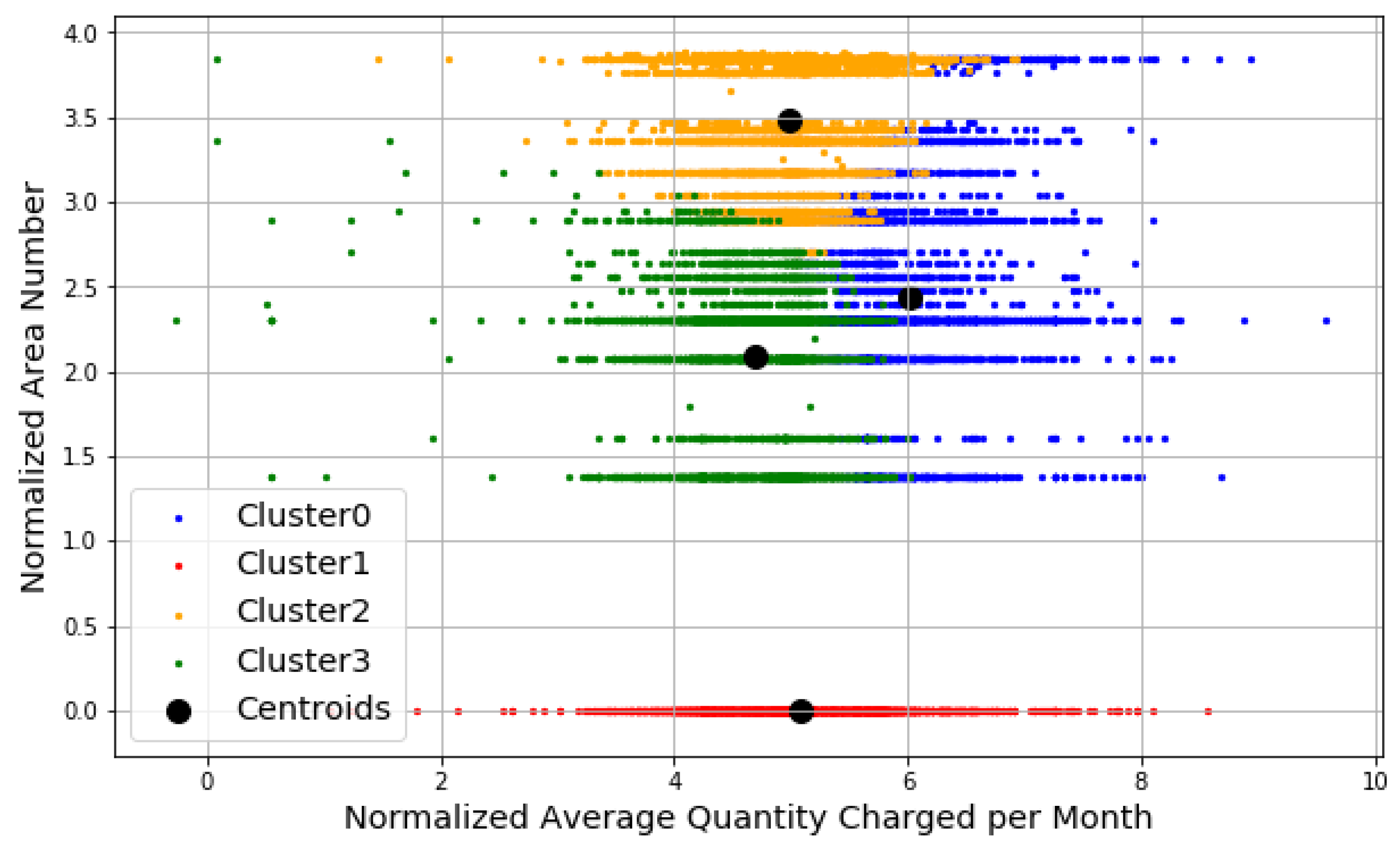
Table 1.
Data set attributes and descriptions.
| Attribute | Description | Format |
|---|---|---|
| BillNo | The bill number of the prepaid smart card charging transaction | Numeric |
| BillDate | The bill date of the prepaid smart card charging transaction | Date |
| ConsumerID | Consumer or user unique ID | String |
| Quantity | The quantity charged in kWh | Numeric |
| Price | The price of 1 KWH | Numeric |
| Hour | The hour of charging smart card | Numeric |
| Period | The period in the day, Evening, Morning, Noon, and Night | String (Evening 6 p.m.–8 p.m., Morning 6 a.m.–10 a.m., Noon 11 a.m.–5 p.m., Night otherwise. |
| Peak | The peak hours during the day are 6 a.m.–10 a.m. and 5 p.m.–8 p.m., or off peak hours otherwise | Numeric (peak-hour = 1, off peak = 2) |
| Day | The day in which the transaction is occurred | Numeric |
| DayofWeek | Weekday | Numeric (Mon = 0 and Sun = 6) |
| WeekEnd | Week end in Palestine is Friday and Saturday, here refers to days before and after Friday the weekend i.e., Thursday and Saturday. | Numeric (Weekend = 1 and 0 otherwise) |
| Month | The month in which the transaction is occurred | Numeric |
| Month-Period | There are 3 months periods June-August is period 1, September-November is period 2, and December is period 3. | Numeric |
| AreaNo | The area number where consumer is located | Numeric (from 1 to 48) |
| TariffNo | Consumers’ Tariff | Numaric (from 1 to 27) |
Table 2.
List of household consumers considered as an outliers.
| ConsumerID | Quantity in kWh per Month | AreaID | Area Name |
|---|---|---|---|
| Y00013083-00143 | 8488.851 | 4 | West |
| Y00010603-00113 | 6831.904 | 1 | Sowth |
| Y00006277-001473 | 5145.798 | 47 | Tulkarm |
| Y00005194-001133 | 5145.798 | 13 | Ezbet Al-Jarad |
| Y00013083-00143 | 5116.638 | 4 | West |
| Y00011015-001473 | 5116.638 | 47 | Tulkarm |
| Y00018491-001103 | 4288.165 | 10 | North |
| Y00011015-001473 | 4288.165 | 47 | Tulkarm |
| Y00015645-00183 | 4087.479 | 8 | East |
Table 3.
Confusion matrix of the support vector machine (SVM).
| Class | 0 | 1 | 2 | 3 |
|---|---|---|---|---|
| 0 | 1351 | 0 | 32 | 26 |
| 1 | 104 | 867 | 0 | 0 |
| 2 | 94 | 0 | 1940 | 9 |
| 3 | 153 | 0 | 11 | 1871 |
© 2019 by the author. Licensee MDPI, Basel, Switzerland. This article is an open access article distributed under the terms and conditions of the Creative Commons Attribution (CC BY) license (http://creativecommons.org/licenses/by/4.0/).
Share and Cite
MDPI and ACS Style
AbuBaker, M. Data Mining Applications in Understanding Electricity Consumers’ Behavior: A Case Study of Tulkarm District, Palestine. Energies 2019, 12, 4287. https://0-doi-org.brum.beds.ac.uk/10.3390/en12224287
AMA Style
AbuBaker M. Data Mining Applications in Understanding Electricity Consumers’ Behavior: A Case Study of Tulkarm District, Palestine. Energies. 2019; 12(22):4287. https://0-doi-org.brum.beds.ac.uk/10.3390/en12224287
Chicago/Turabian StyleAbuBaker, Maher. 2019. "Data Mining Applications in Understanding Electricity Consumers’ Behavior: A Case Study of Tulkarm District, Palestine" Energies 12, no. 22: 4287. https://0-doi-org.brum.beds.ac.uk/10.3390/en12224287
Note that from the first issue of 2016, this journal uses article numbers instead of page numbers. See further details here.