Balancing Generation from Renewable Energy Sources: Profitability of an Energy Trader

Abstract

Motivated by a practical problem faced by an energy trading company in Poland, we investigate the profitability of balancing intermittent generation from renewable energy sources (RES). We consider a company that buys electricity generated by a pool of wind farms and pays their owners the day-ahead system price minus a commission, then sells the actually generated volume in the day-ahead and balancing markets. We evaluate the profitability (measured by the Sharpe ratio) and market risk faced by the energy trader as a function of the commission charged and the adopted trading strategy. We show that publicly available, country-wide RES generation forecasts can be significantly improved using a relatively simple regression model and that trading on this information yields significantly higher profits for the company. Moreover, we address the issue of contract design as a key performance driver. We argue that by offering tolerance range contracts, which transfer some of the risk to wind farm owners, both parties can bilaterally agree on a suitable framework that meets individual risk appetite and profitability expectations.

1. Introduction

Energy markets have gone through a tremendous transition during the last two decades. In the old days, electricity was produced by a few large companies with limited competition and the necessity for short-term load or generation adjustments. Trading was rather a long-term business. The deregulation and liberalization processes that started in the 1990s have led to the introduction of organized market places for short-term electricity trading [1,2,3]. Moreover, under the current European Union climate and energy framework, the energy sector in Europe is in need of extensive modernization. This is especially relevant in Poland, where the generation is still heavily dependent on coal. Of the ca. 45.9 GW of installed capacity at the end of 2018, only ca. 8.6 GW was from renewable energy sources (RES; see https://www.ure.gov.pl).

The dynamic expansion of RES generation (e.g., in Poland from 0.5 to 5.9 GW for wind and from zero to 0.14 GW for solar in the last decade) has had the effect of increasing the volatility of supply. Due to the intermittent and unpredictable nature of wind and solar production, real-time balancing of supply and demand has recently become a more important and complex activity than ever before [4,5,6]. On one hand, this has amplified the importance of intraday markets, which can be used to balance deviations resulting from positions taken in the day-ahead market and the actual demand [7,8,9]. On the other, this has resulted in a situation where—to hedge themselves against the volume risk—utility companies are prepared to pay for wind and solar-generated electricity much less than the day-ahead system price. Actually, in Poland the Renewable Energy Sources Act [10] (Art. 4.1) specifies that small producers (of installed capacity under 10 kW, e.g., a few rooftop PV panels) are guaranteed to be paid for only 80% of generated electricity.

This is where energy traders see their chance to make a profit. If they collect a pool of spatially diversified small RES producers and offer them better financial conditions than a utility company normally would, then both sides can benefit from this situation. This reminds of the virtual power plant (VPP) concept, with a slight difference—VPPs usually integrate several types of dispatchable and non-dispatchable generating units, flexible loads, and storage systems to give a reliable overall power supply [11,12]. In the setup we consider, the generation pool only consists of intermittent sources and does not include loads or storage. All the energy trader can do, is bid the predicted volume in the day-ahead market and trade the remaining energy in the balancing market, typically at a loss. Note, that in contrast to the neighboring German market, in Poland the intraday power market is illiquid and cannot be used to hedge deviations in RES generated volume [13]. This may soon change, however, as in November 2019 Poland started using the XBID model, which allows for cross-border continuous trading of electricity [14].

Hence, the pertinent question is—what is the minimum level of commission charged by the energy trader for the business to be still profitable? And three follow-up questions—what is the risk of running such a business model? Can the trader increase profits by improving the quality of RES generation forecasts? Can the trader maintain the same level of profitability by transferring some of the risk to the wind farm owner, at the cost of charging a lower commission for its services? In this article, we address these issues.

The remainder of the paper is structured as follows. In Section 2 we briefly describe the datasets. In Section 3 we first introduce the benchmark business model, then the alternative trading strategy, which utilizes improved wind generation forecasts. In Section 4 we elaborate on the contract design and introduce tolerance range contracts, which mitigate the extreme risks back to RES producers. In Section 5 we compare the different trading strategies and contract designs in terms of the total profit, Value-at-Risk, and the Sharpe ratio. Finally, in Section 6 we wrap up the results and discuss future directions. Since companies active in the power sector compete in terms of operational excellence and portfolio management capabilities—also via contract design—the presented topic is very current and features high relevance for academics and practitioners alike. To our knowledge, this is the first paper that addresses this important aspect of electricity trading.

2. Datasets

To evaluate the considered trading strategies we use a three-year (1 November 2016–31 October 2019) sample of hourly prices and generation volumes from the Polish power market, see Figure 1 and Figure 2:

• ${\mathit{DA}}_{d,h}$—day-ahead electricity system prices in PLN/MWh (source: TGE S.A., https://tge.pl/statistic-data),
• $B_{d,h}$—balancing market settlement prices in PLN/MWh, i.e., the so-called Imbalance Settlement Prices (in Polish: Cena Rozliczeniowa Odchylenia, CRO; source: PSE S.A., https://www.pse.pl/web/pse-eng/data/balancing-market-operation/settlement-prices),
• ${\widehat{G}}_{d,h}^{WPKD}$—two-days-ahead country-wide wind generation forecasts in MWh, extracted from the Initial Daily Coordination Plan (also called the Two Days Ahead Coordinated Plan; in Polish: Wstȩpny Plan Koordynacyjny Dobowy, WPKD; source: PSE S.A., https://www.pse.pl/web/pse-eng/data/polish-power-system-operation/two-days-ahead-basic-data),
• $G_{d,h}$—actual country-wide wind generation in MWh (source: PSE S.A., https://www.pse.pl/web/pse-eng/data/polish-power-system-operation/generation-in-wind-farms),

where $d=1,\dots ,1095$ is the target day (ranging from 1 November 2016 to 31 October 2019) and $h=1,\dots ,24$ is the target hour. For strategies that require improving generation forecasts, the first year (i.e., 1 November 2016–31 October 2017) will be used for calibrating the predictive model, while the latter two (i.e., 1 November 2017–31 October 2019) for evaluation. Although the benchmark strategy does not require calibration—for consistency—only the latter two years will be used for its evaluation. To put prices denominated in Polish Złoty (PLN) into perspective, let us note that in the last three years the exchange rate oscillated around $1\mathrm{EUR}=4.25\mathrm{PLN}$, with a minimum of ca. 4.10 and a maximum of ca. 4.48 PLN.

3. Trading Strategies

3.1. Assumptions

To define and later evaluate the trading strategies, we have to make some assumptions regarding the energy trader. Firstly, we assume that the company interacts and enters into agreements with small RES producers. Note, that due to data availability we focus on wind generation only. This is not a very restrictive limitation as the installed solar capacity in Poland is still small compared to wind. Furthermore, the pool of wind farms in the company’s portfolio is assumed to be proportional to the country-wide wind generation, both spatially and volume-wise. Its share is equal to U percent of the total generation in Poland. For simplicity we set $U=1\%$, however, this is not a limitation as the results scale linearly with U.

Secondly, we assume that the company buys all of the electricity produced by the RES units in its portfolio and the contracts are structured in such a way that the trader pays the day-ahead price ${DA}_{d,h}$ minus a fixed commission C for every MWh generated. Thirdly, that the trader is a price taker and its impact on imbalance volumes and prices are negligible. Finally, we do not take into account transaction costs, since they are dependent on individual bilateral agreements between clearing banks, exchanges, and energy traders, and may vary.

3.2. The Benchmark Strategy

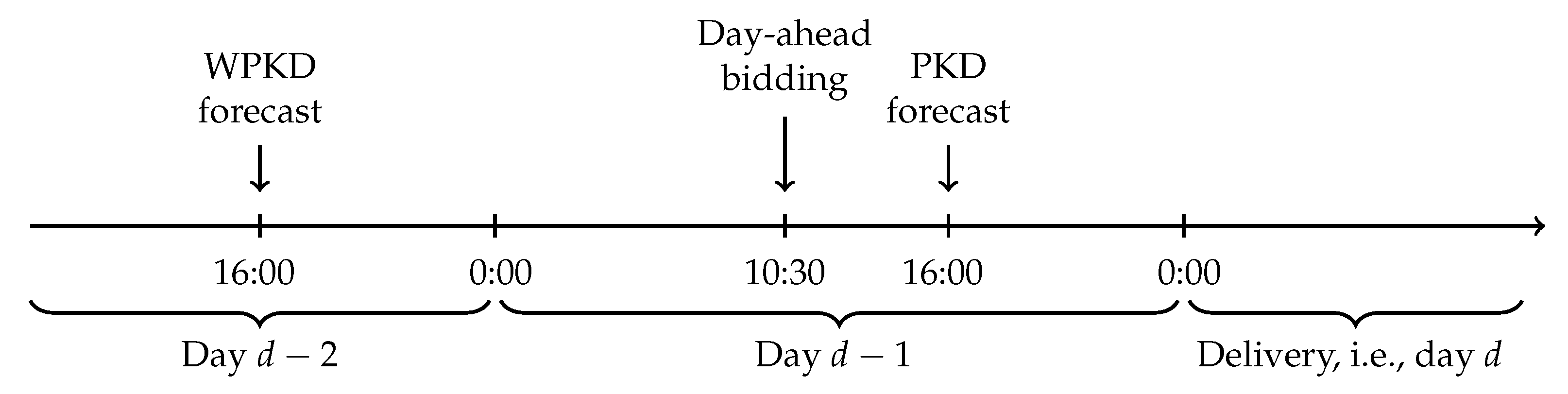
The benchmark strategy is based on data freely available to all market participants and a simple decision rule. Namely, as the country-wide wind generation forecasts ${\widehat{G}}_{d,h}^{\mathit{WPKD}}$ extracted from the Initial Daily Coordination Plan (i.e., WPKD) are published in the afternoon of day $d-2$, they can be used when bidding in the day-ahead market, i.e., before 10:30 on day $d-1$, see Figure 3. The decision rule is: bid the WPKD-predicted volume in the day-ahead market, then buy/sell the residual volume in the balancing market. More precisely, the benchmark strategy is as follows:

• Before 10:30 on day $d-1$, the trader bids a volume of ${\widehat{G}}_{d,h}^{\mathit{WPKD}}\times U$ in the day-ahead market, at the minimum price. Note, that there is no risk of not accepting such bids. Hence, we can interpret that de facto the company sells this volume at the day-ahead price ${\mathit{DA}}_{d,h}$ PLN/MWh.
• On day d, the company sells (if positive) or buys (if negative) the residual volume:

  $${\mathit{Res}}_{d,h}=\left(G_{d,h}-{\widehat{G}}_{d,h}^{\mathit{WPKD}}\right)\times U\mathrm{MWh},$$

  (1)

  in the balancing market at the CRO price $B_{d,h}$ PLN/MWh.

For the whole generated volume, i.e., $G_{d,h}\times U$, the company charges a fixed commission of C PLN/MWh. Hence, the profit (or loss) of the energy trader for day d and hour h is given by

$$P_{d,h}=\left\{(B_{d,h}-{\mathit{DA}}_{d,h})\times \left(G_{d,h}-{\widehat{G}}_{d,h}^{\mathit{WPKD}}\right)+C\times G_{d,h}\right\}\times U.$$

(2)

3.3. Trading on Improved Wind Generation Forecasts

The benchmark strategy relies on relatively inaccurate two-days-ahead (i.e., WPKD) wind generation forecasts. What would be the financial outcome if we used better predictions? Firstly, let us note that perfect or crystal ball predictions, i.e., ${\widehat{G}}_{d,h}^{\mathit{perfect}}\equiv G_{d,h}$, would lead to selling the whole production in the day-ahead market at ${\mathit{DA}}_{d,h}$ PLN/MWh and paying exactly the same price to the RES generators. Consequently, the profit would be

$$P_{d,h}^{\mathit{perfect}}=C\times G_{d,h}\times U.$$

(3)

If better than WPKD but worse than perfect forecasts were used, then the financial outcome could be different. Unfortunately, the more up-to-date Daily Coordination Plan (also called the Day Ahead Coordinated Plan; in Polish: Plan Koordynacyjny Dobowy, PKD) is published by PSE S.A. at 16:00 on day $d-1$, see Figure 3, too late to be taken into account in the decision process. Hence, we take an alternative approach and—following the recent works of Maciejowska et al. [13,15]—use a regression-type model to improve on WPKD forecasts. Then we let the improved predictions ${\widehat{G}}_{d,h}^{\mathit{Imp}}$ define the volume of bids submitted to the power exchange.

More precisely, we model the country-wide wind generation by the following formula:

$$G_{d,h}={\beta }_{h,0}+{\beta }_{h,1}{G}_{d-1,h}^{*}+{\beta }_{h,2}{\widehat{G}}_{d,h}^{\mathit{WPKD}}+{\beta }_{h,3}{\widehat{G}}_{d,ave}^{\mathit{WPKD}}+{\epsilon }_{d,h},$$

(4)

where independently for each hour h. Here, ${\beta }_{h,0},\dots ,{\beta }_{h,3}$ are the coefficients, ${\widehat{G}}_{d,h}^{\mathit{WPKD}}$ is the WPKD forecast for the current day and hour, ${\widehat{G}}_{d,ave}^{\mathit{WPKD}}$ is its average across all 24 hours of day d and ${\epsilon }_{d,h}$ is the noise term. Note, that at the time the trading decision has to be made, i.e., before 10:30 on day $d-1$, the actual wind generation is unknown for hours $h>10$. Hence, we define the autoregressive term as

$$G_{d-1,h}^{*}=\left\{\begin{array}{c}{G}_{d-1,h}\mathrm{if}h\le 10,\hfill \\ {\widehat{G}}_{d-1,h}^{\mathit{WPKD}}\mathrm{if}h>10,\hfill \end{array}\right.$$

(5)

which replaces the unknown observations with their WPKD forecasts for day $d-1$.

The model defined by Equation (4) is estimated using least squares for different lengths of the calibration window. Then the predictions are averaged across the calibration windows, as originally proposed by Hubicka et al. [16]. Based on a limited simulation study and empirical evidence presented in [16,17,18], we use six short windows of $\tau \in \{56,82,108,134,160,186\}$ days, which range from two to six months of past data, and six long windows of $\tau \in \{330,337,344,351,358,365\}$ days, which balance the short term effect. The improved country-wide wind generation forecasts are then computed as a simple arithmetic average over the 12 individual predictions obtained for $\tau \in \{56,82,\dots ,365\}$, adjusted by the mean error of the WPKD forecasts from the previous year and with a lower bound at zero:

$${\widehat{G}}_{d,h}^{\mathit{Imp}}\equiv max\left\{\underset{\mathrm{ensemble}\mathrm{forecast}}{\underbrace{\frac{1}{12}\sum _{\tau \in \{56,82,\dots ,365\}}{\widehat{G}}_{d,h}^{\tau }}}-\underset{\mathrm{WPKD}\mathrm{adjustment}}{\underbrace{\frac{1}{364}\sum _{i=d-365}^{d-2}\left(G_{i,h}-{\widehat{G}}_{i,h}^{\mathit{WPKD}}\right)}};0\right\},$$

(6)

where ${\widehat{G}}_{d,h}^{\tau }$ is the forecast obtained for model (4) using calibration window of length $\tau$. Note, that the improved forecasts are computed independently for each hour, hence h is fixed in the above formula.

The WPKD adjustment is required for the improved forecasts to be at par with ${\widehat{G}}_{i,h}^{\mathit{WPKD}}$, which—on average—consistently underestimate the actual wind generation volume. Given that the balancing prices in Poland are generally higher than in the day-ahead market, a company trading on WPKD predictions would achieve higher profits than when using more accurate, but on average higher improved forecasts, simply because it would sell more in the balancing market. Finally, the lower bound at zero is there to ensure that ${\widehat{G}}_{d,h}^{\mathit{Imp}}$ is non-negative. Since we are considering wind generation volumes, negative values would not make sense.

4. Contract Design

4.1. The Importance of Contract Design for Financial Performance and Risk Mitigation

In Section 3 our main concern was the trading strategy. However, the contract design itself is a key performance driver as well. The perception of risk and volatility in trading even found its way into best-selling book lists. As Taleb [19] argues, traders frequently underestimate extreme tail events causing entire businesses to go bankrupt. A core message is to expect the unexpected, i.e., expect statistical outliers even beyond your initial sample. While this is a more time-series related argumentation, there is also the omnipresent risk of regime-switches. In particular, the balancing market regulations have changed in the European countries quite frequently in the past and are likely to do so in the near future [20,21]. Given this, an energy trader has two options—accept the full risk for a considerable premium on the commission or mitigate risks by specific contract design, e.g., by transferring risks related to extreme price scenarios back to the RES producers. Such risk-mitigating contracts may be viewed as a chance for the generators since they do not have to pay an additional insurance fee for the extreme events that might never come.

For the sake of completeness, we do not want to leave another option unmentioned. If the RES producer is—based on market expectations—willing to accept the entire price risk, i.e., pay the imbalance costs, then no risk mitigation or specific contract design is required. This approach reduces the relationship between an energy trader and a RES producer to a service level agreement in which the energy trader carries out operational tasks, like TSO nomination. As these contracts do not require any price-based computation, we do not discuss them any further in this paper.

4.2. Unrestricted Contracts

The simplest form of a RES-based Power Purchase Agreement (PPA) is an unrestricted contract. It confirms the willingness of an energy trader to take over the entire volume and price risk. The trader is responsible for the respective bidding strategy. Based on generation forecasts, volumes will be sold in day-ahead markets. However, it will be inevitable that the deviation between the generation forecast and the actual generation will be settled in imbalance markets. This settlement adds uncertainty about the actual imbalance price ${\mathit{B}}_{\mathit{d},\mathit{h}}$ to the expected profit of the energy trader, see Equation (2).

That being said, an unrestricted contract works like a fully comprehensive cover. It features no limitation of imbalance price liability. The RES producer does not have to care about generation forecast accuracy or imbalance prices anymore. On the other hand, the energy trader takes the full risk of regime-switches or extreme price movements of ${\mathit{B}}_{\mathit{d},\mathit{h}}$. Unrestricted contracts are usually more costly for RES producers than their restricted equivalents, however, they are perfectly suited for generators that need constant and predictable cash-flows for investment decisions and have a very low-risk appetite. For instance, a consortium of investors willing to build a wind farm may evaluate profitability based on cash-flows over the next 20 or even 30 years. Their investment decisions are less complex if they can mitigate as many risks as possible and swap concerns about imbalance price spikes for a higher commission [22,23].

4.3. Tolerance Range Contracts

An alternative to unrestricted contracts are agreements which transfer the risks related to extreme price scenarios back to the RES producers [24,25]. In such contracts, traders define a tolerance range in which they pay ${\mathit{DA}}_{d,h}$ to asset owners. In financial terms, this means that the profit is no longer given by Equation (2) but becomes:

$$P_{d,h}=\left\{\begin{array}{cc}\left\{(B_{d,h}-{\mathit{DA}}_{d,h})\times \left(G_{d,h}-{\widehat{G}}_{d,h}^{\mathit{WPKD}}\right)+C\times G_{d,h}\right\}\times U\hfill & \mathrm{for}\left|B_{d,h}-D{A}_{d,h}\right|<T_{d,h},\hfill \\ 0\hfill & \mathrm{otherwise},\hfill \end{array}\right.$$

(7)

where ${\mathit{T}}_{\mathit{d},\mathit{h}}$ is the tolerance threshold in PLN/MWh, potentially set for each hour independently. The latter defines the range of imbalance prices in which the energy trader takes over the imbalance risk. Outside of that range, the generator has to cover any imbalance costs that arise (but does not have to pay the commission). This risk mitigation oriented contract design allows one to hedge extreme price events and works like an inverted insurance policy with a voluntary excess. The only difference to the well-known concept in the insurance world is that the RES producer does not receive a small fee at the time the event occurs (like a writer of a voluntary excess policy would), but accepts the whole risk in case of extreme price events. Seen from the other side, the tolerance range contract does not generate profits for the energy trader if $|B_{d,h}-D{A}_{d,h}|\ge T_{d,h}$, but protects the trader against losses under such business threatening scenarios.

The threshold ${\mathit{T}}_{\mathit{d},\mathit{h}}$ can be determined in multiple ways. One could argue for using empirical quantiles of ${\mathit{B}}_{d,h}$. However, this approach bears a risk. The main idea of a tolerance range contract is to prepare for the unexpected. Hence, a derivation based on historical distributions implies that nothing worse than in the past can occur. Only using quantiles of ${\mathit{B}}_{d,h}$ could lead to biased decision making since the ratio between day-ahead and imbalance markets is the one that matters for the pay-off of the contract. If the imbalance price reaches high levels and the day-ahead price does so as well, the impact on the profits will not be as extreme as an isolated view on quantiles suggests. Therefore, we propose an approach that bears in mind the limited informative content of past values and the spread characteristics of the pay-off structure. Using the absolute difference between day-ahead and imbalance prices $|B_{d,h}-D{A}_{d,h}|$ as the threshold determinant allows the energy trader to effortlessly adjust the contract based on the willingness to accept risk. Another advantage of the absolute difference or the spread between day-ahead and imbalance prices is its simplicity that allows senior managers or potential customers to grasp its meaning without any statistical knowledge or the necessity to have a formula in front of them.

5. Results

5.1. Evaluation Metrics

We will evaluate the different strategies and contract designs using three types of metrics, for a range of C and $T_{d,h}$ values. The first type includes two simple statistics – the total and cumulative profits. The former is defined as a sum of $P_{d,h}$ across all days d and all (or selected) hours h in the evaluation period $\mathcal{T}$, while the latter as a sum across all (or selected) hours from day one (in the evaluation period) up to a certain day, say, $d^{*}$. The second is a Value-at-Risk type measure [26]. Mathematically, it is a quantile of the (empirical) distribution of the daily profit $P_d={\sum }_{h=1}^{24}{P}_{d,h}$ in the evaluation period $\mathcal{T}$. We will denote it by ${\mathit{VaR}}_{1-q}$, where q is the quantile level, e.g., $q=5\%$. Finally, we will also look at a well-known criterion for portfolio performance evaluation, namely the Sharpe ratio [26]:

$$SR=\frac{\frac{1}{\#\mathcal{T}}{\sum }_{d\in \mathcal{T}}{P}_d}{{\sigma }_d},$$

(8)

where $\#\mathcal{T}$ is the number of days in $\mathcal{T}$ and ${\sigma }_d$ is the standard deviation of $P_d$ in the evaluation period. Note, that in the original formulation of the Sharpe ratio, the performance of the investment is compared to the returns of a risk-free instrument. However, here we follow [8,27] and assume a zero risk-free rate, so that the realized profits are identical to the relative portfolio returns.

5.2. Total and Cumulative Profits

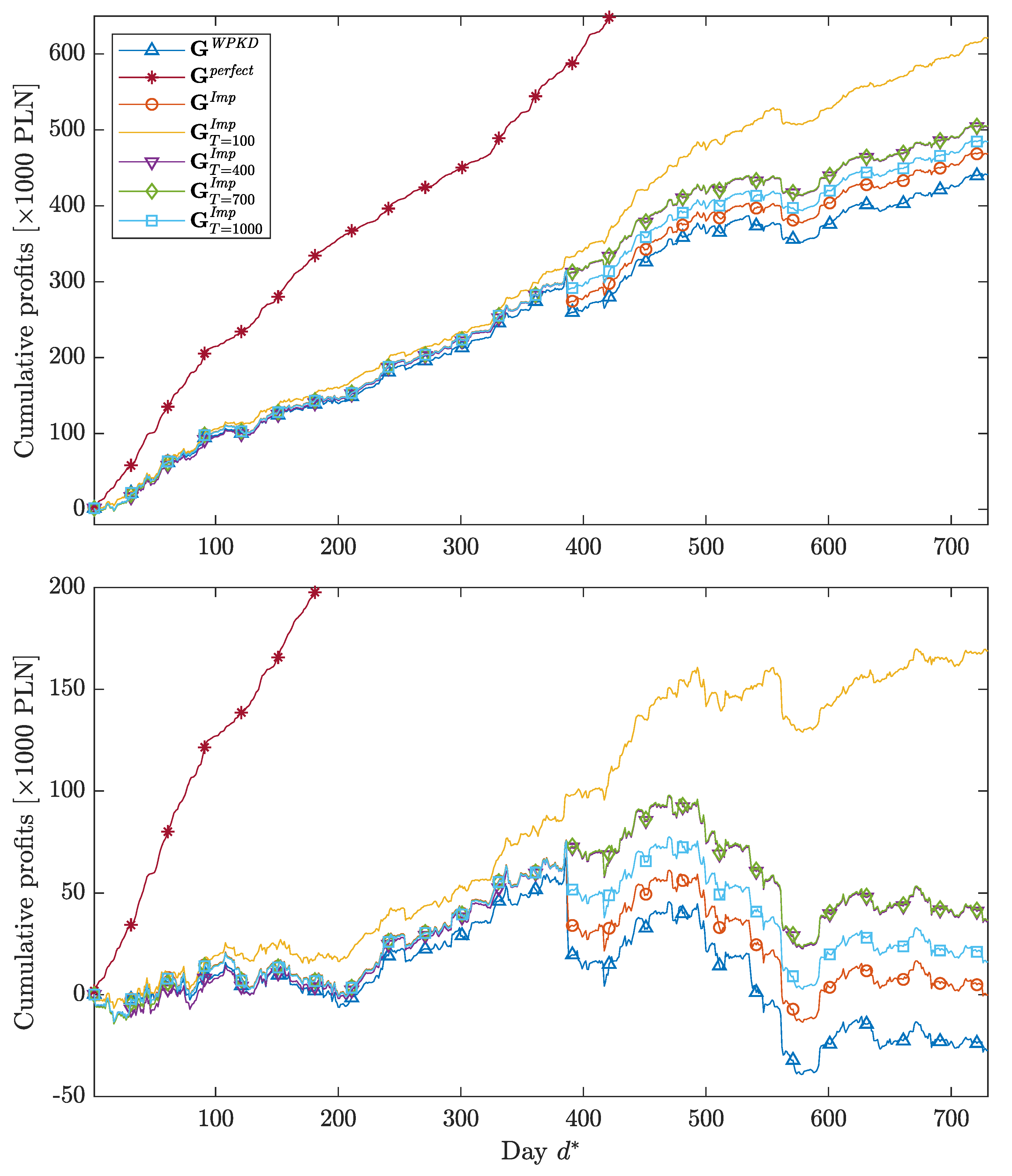
Let us now look at the total and cumulative profits for two benchmark strategies and two types of trading strategies utilizing improved wind generation forecasts:

• the benchmark strategy—denoted by ${\mathbf{G}}^{\mathit{WPKD}}$—based on unrestricted contracts (see Section 4.2) and WPKD forecasts (see Section 3.2),
• the crystal ball strategy—denoted by ${\mathbf{G}}^{\mathit{perfect}}$—based on perfect wind generation forecasts (see Equation (3) in Section 3.3) instead of WPKD predictions,
• a strategy—denoted by ${\mathbf{G}}^{\mathit{Imp}}$—utilizing improved wind generation forecasts (see Section 3.3) instead of WPKD predictions,
• strategies—denoted by ${\mathbf{G}}_T^{\mathit{WPKD}}$ or ${\mathbf{G}}_T^{\mathit{Imp}}$ —based on tolerance range contracts for a range of tolerance thresholds $T=100,\dots ,1300$ (see Section 4.3), respectively utilizing the WPKD or improved wind generation forecasts.

For simplicity, we assume that the tolerance threshold is the same for all days and hours in the evaluation period, i.e., $T=T_{d,h}$. However, this restriction can be easily lifted.

The total profits for the different strategies considered and the whole two-year out-of-sample evaluation period are summarized in

Table 1. Comparison of total profits for the different strategies considered and the whole two-year out-of-sample evaluation period, see Figure 1 and Figure 2. Two values of C are emphasized in bold: 2.51 PLN, which yields a zero profit for the ${\mathbf{G}}^{\mathit{Imp}}$ strategy, and 1 EUR ≈ 4.25 PLN.

Commission	Strategy
C [PLN]	${\mathbf{G}}^{\mathit{WPKD}}$	${\mathbf{G}}^{\mathit{perfect}}$	${\mathbf{G}}^{\mathit{Imp}}$	${\mathbf{G}}_{\mathit{T}=100}^{\mathit{Imp}}$	${\mathbf{G}}_{\mathit{T}=400}^{\mathit{Imp}}$	${\mathbf{G}}_{\mathit{T}=700}^{\mathit{Imp}}$	${\mathbf{G}}_{\mathit{T}=1000}^{\mathit{Imp}}$
0.00	−705,573	0	−678,294	−485,524	−641,585	−641,220	−661,914
1.00	−435,664	269,909	−408,385	−225,058	−371,924	−371,432	−392,065
2.00	−165,755	539,818	−138,476	35,408	−102,264	−101,644	−122,216
2.51	−27,279	678,293	0	169,038	36,084	36,769	16,228
3.00	104,154	809,727	131,433	295,874	167,397	168,144	147,633
1 EUR ≈ 4.25	441,540	1,147,113	468,819	621,456	504,473	505,379	484,944
5.00	643,972	1,349,545	671,250	816,806	706,719	707,720	687,331

. We can see that the strategy utilizing improved wind generation forecasts outperforms the benchmark strategy by ca. 27 thousand PLN. The break even commission is somewhere between 2 and 3 PLN, except for the crystal ball strategy (which has a break even point at $C=0$ PLN) and the tolerance range contract with threshold $T=100$ PLN. The latter also leads to significantly higher profits than ${\mathbf{G}}^{\mathit{WPKD}}$ and ${\mathbf{G}}^{\mathit{Imp}}$. The downside of this is that a lower commission will most likely be negotiated with the RES producers as a substantial part of the risk is transferred to them. Interestingly, there is almost no difference between the ${\mathbf{G}}_{T=400}^{\mathit{Imp}}$ and ${\mathbf{G}}_{T=700}^{\mathit{Imp}}$ strategies, actually the latter is slightly more profitable. This suggests that there are ranges of tolerance threshold values that yield nearly identical outcomes but provide different negotiation grounds. Naturally, a higher commission can be achieved for higher thresholds.

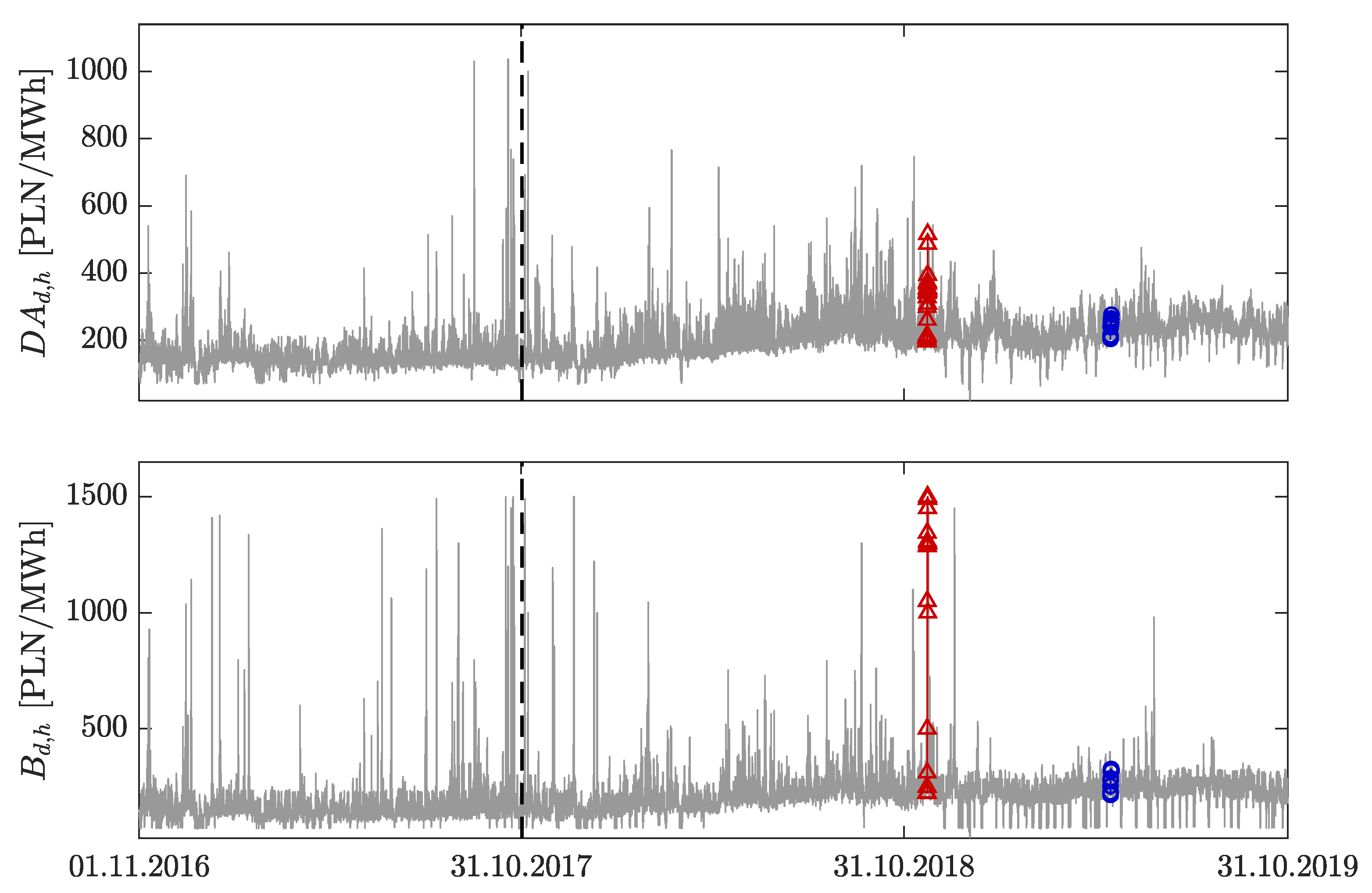
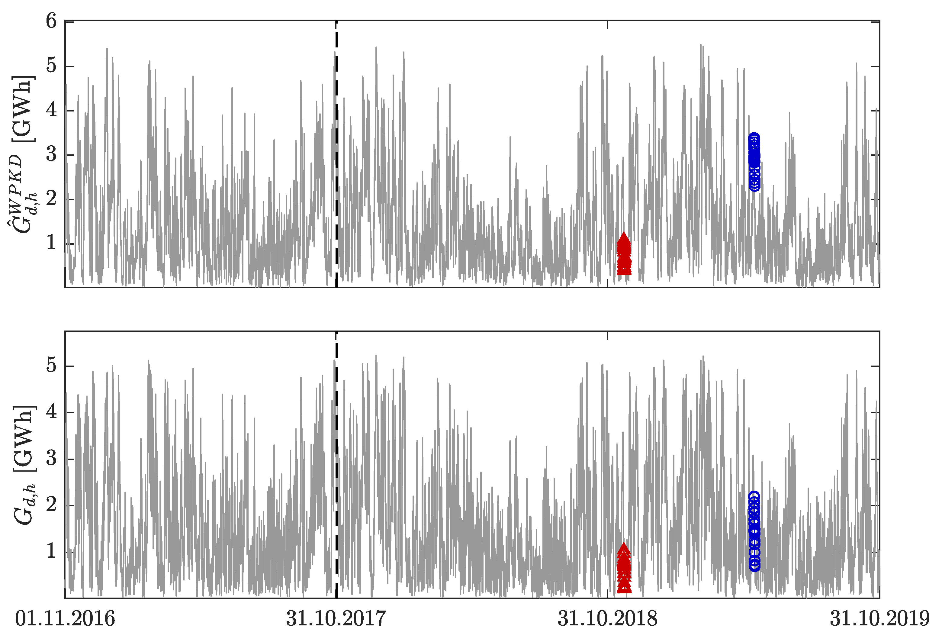
What is important, the profits from this line of business are persistent—see Figure 4 illustrating cumulative profits for the different strategies considered—although with a few draw-downs. As expected, the losses are more severe for unrestricted contracts and tolerance range contracts with large thresholds. The largest draw-down in profits for the unrestricted contract strategies occurred on 22.11.2018 ($d^{*}=387$), when wind generation for hours 15–21 was much lower than predicted and balancing prices spiked, see the red triangles in Figure 1 and Figure 2. Nevertheless, ${\mathbf{G}}^{\mathit{Imp}}$ fared much better than ${\mathbf{G}}^{\mathit{WPKD}}$, its daily loss for commission level $C=4.25$ PLN was $-\mathrm{29,790}$ PLN compared to $-\mathrm{34,115}$ PLN for the benchmark. Note, that the ${\mathbf{G}}_T^{\mathit{Imp}}$ strategies were largely immunized by the tolerance threshold. The second-largest draw-down—this time influencing all strategies—occurred on 16.05.2019 ($d^{*}=562$), when wind generation was largely overestimated for all hours of the day, but balancing and day-ahead prices stayed similar, see the blue circles in Figure 1 and Figure 2.

Finally, note that in Figure 4 we are comparing strategies based on only one commission level, i.e., $C=4.25$ PLN (upper panel) or $C=2.51$ PLN (lower panel), as using different levels for different contracts would require assumptions on the terms of the individual bilateral agreements. Hence, we cannot simply say that ${\mathbf{G}}_{T=700}^{\mathit{Imp}}$ is more profitable than ${\mathbf{G}}^{\mathit{Imp}}$, because we do not know what would be the difference between the commissions negotiated on such contracts.

5.3. Value-at-Risk

Let us now focus on the risk borne by the energy trader. In

Table 2. Comparison of daily $Va{R}_{95\%}$ values for the different strategies considered and the whole two-year out-of-sample evaluation period, see Figure 1 and Figure 2. Two values of C are emphasized in bold: 2.51 PLN, which yields a zero profit for the ${\mathbf{G}}^{\mathit{Imp}}$ strategy (see Table 1), and 1 EUR ≈ 4.25 PLN.

Commission	Strategy
C [PLN]	${\mathbf{G}}^{\mathit{WPKD}}$	${\mathbf{G}}^{\mathit{perfect}}$	${\mathbf{G}}^{\mathit{Imp}}$	${\mathbf{G}}_{\mathit{T}=100}^{\mathit{Imp}}$	${\mathbf{G}}_{\mathit{T}=400}^{\mathit{Imp}}$	${\mathit{G}}_{\mathit{T}=700}^{\mathbf{Imp}}$	${\mathit{G}}_{\mathit{T}=1000}^{\mathbf{Imp}}$
0.00	−4803	0	−4465	−3535	−4424	−4445	−4465
1.00	−4305	78	−4046	−2979	−3934	−3930	−4046
2.00	−3865	156	−3705	−2408	−3449	−3449	−3705
2.51	−3697	196	−3562	−2158	−3379	−3379	−3562
3.00	−3515	235	−3406	−1927	−3254	−3254	−3406
1 EUR ≈ 4.25	−3034	333	−2883	−1468	−2514	−2 725	−2883
5.00	−2786	391	−2666	−1179	−2184	−2333	−2666

we report the daily $Va{R}_{95\%}$ values, see Section 5.1, for the different strategies considered and the whole two-year out-of-sample evaluation period. The picture is similar to that in Table 1. The daily $Va{R}_{95\%}$ is more negative for ${\mathbf{G}}^{\mathit{WPKD}}$ than for ${\mathbf{G}}^{\mathit{Imp}}$, which is more negative than for ${\mathbf{G}}_T^{\mathit{Imp}}$ with $T=100,400$, and 700 PLN. Interestingly, the profit and loss (P/L) distribution for the ${\mathbf{G}}_{T=1000}^{\mathit{Imp}}$ strategy has the same 5% quantile as ${\mathbf{G}}^{\mathit{Imp}}$.

The energy trader may be interested in setting the commission level so that the daily $Va{R}_{95\%}$ does not exceed a certain threshold. With this in mind, in Figure 5 we plot C as a function of $Va{R}_{95\%}$. For instance, if a daily ${\mathrm{VaR}}_{95\%}$ of $-4000$ PLN is acceptable for the company, then the minimum commission the company can charge is 1.49 PLN when using the ${\mathbf{G}}^{\mathit{WPKD}}$ strategy and 0.99 PLN when utilizing the improved forecasts (see the leftmost square and circle, respectively). However, when a negative P/L is acceptable on only 5% of days, then the commission has to be in excess of 14.05 PLN for WPKD forecasts and 13.75 PLN for improved forecasts (see the rightmost values in the plot).

5.4. Sharpe Ratios

A higher total or cumulative profit is not necessarily a good indicator of a profitable strategy, as it neglects the risk borne by the energy trader. On the other hand, the Sharpe ratio introduced in Equation (8) does not possess this draw-down. It reflects the trade-off between maximizing profits and minimizing their variance.

In Figure 6 we plot the Sharpe ratio as a function of the tolerance threshold $T=T_{d,h}$; note, that all computations involve one and the same commission level of $C=4.25$ PLN. Clearly, the lower the tolerance threshold, i.e., the more risk is transferred to the RES producer, the higher the Sharpe ratio. However, the relationship is not linear. The Sharpe ratio decays approximately exponentially between $T=100$ and 300 PLN, then stays practically constant up to $T=900$ PLN, then decays in a stepwise fashion until $T=1150$ PLN and finally stays constant. In other words, the profitability is roughly the same for a wide range of thresholds—from $T=300$ to 900 PLN—a phenomenon already visible to some extent in Table 1. This non-linearity is most likely caused by the underlying price spread between day-ahead and imbalance prices. Taking a closer look at Figure 1 we can clearly see the mean-reverting character of electricity prices. Generally, the prices stay in the “normal” regime, but once in a while, they spike, then quickly return to the previous level [1]. This effect translates into a Sharpe ratio which is stable for a wide range of Ts, but rapidly changes in the tails, i.e., in the areas where we observe extreme prices.

The above observation provides valuable insights for contract negotiators, who can charge a higher commission for $T=900$ PLN without accepting any more risk than for $T=300$ PLN. Note also, that the ${\mathbf{G}}_T^{\mathit{Imp}}$ strategies are more profitable than the corresponding ${\mathbf{G}}_T^{\mathit{WPKD}}$ strategies for the whole range of tolerance thresholds considered, justifying the approach introduced in Section 3.3.

6. Summary and Outlook

6.1. Conclusions

Managing a RES portfolio is one of the major challenges for modern energy traders in Europe. Investors, stipulated by new government guidelines, seek to build new wind farms and consequently are looking for commercial partners that offer suitable agreements. In this paper, we have discussed two major aspects that are crucial for the overall performance from an energy trader’s perspective. Firstly, we have shown, based on the example of the Polish power market, that traders can substantially increase their profitability by utilizing RES generation forecasts of higher quality. To this end, we have proposed a parsimonious linear regression model that uses publicly available data (WPKD wind generation forecasts of the system operator and past wind generation figures) to model the country-wide wind generation. Our approach outperforms the benchmark strategy based on WPKD predictions and yields significantly higher profits for the energy trader. Hence, we also contribute to a relatively new and important area of energy research, which focuses on the economic benefits of improved forecasts instead of the prediction errors themselves [8,13].

Secondly, we have addressed the issue of contract design as another key performance driver. While energy traders can improve their profitability with advanced forecasting techniques, they can hardly predict future policy changes or very extreme price movements. Since these events are a considerable threat to profitability, we consider a viable way to mitigate these risks. Instead of signing unrestricted contracts where the energy traders take all the risk, they can negotiate tolerance range contracts where the extreme tail events are to be paid by the RES producers. We suggest considering absolute price spreads between the day-ahead and imbalance markets as the contractual anchor point and demonstrate that a tolerance range based on this spread helps to increase the profitability and the Sharpe ratio. At the same time, it allows one to reduce the commission, which leaves both the RES producer and the energy trader with more flexibility in their contract design. Within such a contract design, they can bilaterally agree on a suitable framework based on individual risk appetite and profitability expectations. We believe that this is an important aspect that will increase commercial interest in RES investment projects.

6.2. Future Directions

We should also emphasize that in this study we are using only one, relatively simple way of improving wind generation forecasts. More complex approaches, like LASSO [9,28] or deep learning [29,30], and the addition of other exogenous variables, like power plant availability, control area balances or updated forecasts of RES generation [7], can be easily addressed in future work. Instead of using point predictions, one could improve the spot trading activities based on probabilities instead of the expected outcome alone [31,32]. Besides the methodological extensions, future research could also address practical aspects of RES-related contracts more prominently. We have made the first step by considering contract design issues. However, there are many more aspects to be taken into account. For instance, how should risk mitigation be considered in the active promotion of RES-related trading contracts? How should the flexibility in contract design be added to long-term evaluations of wind farm projects? Last but not least, we want to emphasize that the Polish market discussed in this paper features limited liquidity in intraday trading, which is why we have neglected this facet of RES portfolio management. It could be beneficial to transfer our considerations to a market with more liquid intraday trading activities and evaluate how decision making in these markets affects profitability. However, such an analysis would require both intraday RES generation forecasts and order book data.

References

- Weron, R. Electricity price forecasting: A review of the state-of-the-art with a look into the future. Int. J. Forecast. 2014, 30, 1030–1081. [Google Scholar] [CrossRef] [Green Version]
- Viehmann, J. State of the German short-term power market. Zeitschrift für Energiewirtschaft 2017, 41, 87–103. [Google Scholar] [CrossRef]
- Mayer, K.; Trück, S. Electricity markets around the world. J. Commod. Mark. 2018, 9, 77–100. [Google Scholar] [CrossRef]
- Gianfreda, A.; Parisio, L.; Pelagatti, M. The impact of RES in the Italian day-ahead and balancing markets. Energy J. 2016, 37, 161–184. [Google Scholar]
- Cole, W.; Frazier, A. Impacts of increasing penetration of renewable energy on the operation of the power sector. Electr. J. 2018, 31, 24–31. [Google Scholar] [CrossRef]
- Maciejowska, K. Assessing the impact of renewable energy sources on the electricity price level and variability—A Quantile Regression approach. Energy Econ. 2020, 85, 104532. [Google Scholar] [CrossRef]
- Kiesel, R.; Paraschiv, F. Econometric analysis of 15-minute intraday electricity prices. Energy Econ. 2017, 64, 77–90. [Google Scholar] [CrossRef] [Green Version]
- Kath, C.; Ziel, F. The value of forecasts: Quantifying the economic gains of accurate quarter-hourly electricity price forecasts. Energy Econ. 2018, 76, 411–423. [Google Scholar] [CrossRef] [Green Version]
- Uniejewski, B.; Marcjasz, G.; Weron, R. Understanding intraday electricity markets: Variable selection and very short-term price forecasting using LASSO. Int. J. Forecast. 2019, 35, 1533–1547. [Google Scholar] [CrossRef] [Green Version]
- Renewable Energy Sources Act of 20 February 2015. Republic of Poland, Dz.U. 2015 poz. 478 and Later Amendments. 2015. Available online: http://prawo.sejm.gov.pl/isap.nsf/DocDetails.xsp?id=WDU20150000478 (accessed on 20 February 2015).
- Morales, J.M.; Conejo, A.J.; Madsen, H.; Pinson, P.; Zugno, M. Integrating Renewables in Electricity Markets: Operational Problems; Springer: New York, NY, USA, 2014. [Google Scholar]
- Sikorski, T.; Jasiński, M.; Ropuszyńska-Surma, E.; Wȩglarz, M.; Kaczorowska, D.; Kostyła, P.; Leonowicz, Z.; Lis, R.; Rezmer, J.; Rojewski, W.; et al. A case study on distributed energy resources and energy-storage systems in a Virtual Power Plant concept: Economic aspects. Energies 2019, 12, 4447. [Google Scholar] [CrossRef] [Green Version]
- Maciejowska, K.; Nitka, W.; Weron, T. Day-ahead vs. Intraday—Forecasting the price spread to maximize economic benefits. Energies 2019, 12, 631. [Google Scholar] [CrossRef] [Green Version]
- Kath, C. Modeling intraday markets under the new advances of the cross-border intraday project (XBID): Evidence from the German intraday market. Energies 2019, 12, 4339. [Google Scholar] [CrossRef] [Green Version]
- Maciejowska, K.; Nitka, W.; Weron, T. Enhancing load, wind and solar generation forecasts in day-ahead forecasting of spot and intraday electricity prices. Energy Econ. 2019. submitted. [Google Scholar]
- Hubicka, K.; Marcjasz, G.; Weron, R. A note on averaging day-ahead electricity price forecasts across calibration windows. IEEE Trans. Sustain. Energy 2019, 10, 321–323. [Google Scholar] [CrossRef]
- Marcjasz, G.; Serafin, T.; Weron, R. Selection of calibration windows for day-ahead electricity price forecasting. Energies 2018, 11, 2364. [Google Scholar] [CrossRef] [Green Version]
- Serafin, T.; Uniejewski, B.; Weron, R. Averaging predictive distributions across calibration windows for day-ahead electricity price forecasting. Energies 2019, 12, 2561. [Google Scholar] [CrossRef] [Green Version]
- Taleb, N. Fooled by Randomness: The Hidden Role of Chance in Life and in the Markets; Random House: New York, NY, USA, 2005. [Google Scholar]
- Zaleski, P.; Klimczak, D. Prospects for the rise of renewable sources of energy in Poland. Balancing renewables on the intra-day market. In Capacity Market in Contemporary Economic Policy; Zamasz, K., Ed.; Difin: Warszawa, Poland, 2015; pp. 124–138. [Google Scholar]
- Koch, C.; Hirth, L. Short-term electricity trading for system balancing: An empirical analysis of the role of intraday trading in balancing Germany’s electricity system. Renew. Sustain. Energy Rev. 2019, 113, 109275. [Google Scholar] [CrossRef] [Green Version]
- Blanco, M.I. The economics of wind energy. Renew. Sustain. Energy Rev. 2009, 13, 1372–1382. [Google Scholar] [CrossRef]
- Dicorato, M.; Forte, G.; Pisani, M.; Trovato, M. Guidelines for assessment of investment cost for offshore wind generation. Renew. Energy 2011, 36, 2043–2051. [Google Scholar] [CrossRef]
- Tavafoghi, H.; Teneketzis, D. Optimal contract design for energy procurement. In Proceedings of the 52nd Annual Allerton Conference on Communication, Control, and Computing, Monticello, IL, USA, 1–3 October 2014. [Google Scholar] [CrossRef]
- Bruck, M.; Sandborn, P.; Goudarzi, N. A Levelized Cost of Energy (LCOE) model for wind farms that include Power Purchase Agreements (PPAs). Renew. Energy 2018, 122, 131–139. [Google Scholar] [CrossRef]
- Alexander, C. Market Risk Analysis; Wiley: Chichester, UK, 2008; Volume I–IV. [Google Scholar]
- Baltaoglu, S.; Tong, L.; Zhao, Q. Algorithmic bidding for virtual trading in electricity markets. IEEE Trans. Power Syst. 2019, 34, 535–543. [Google Scholar]
- Narajewski, M.; Ziel, F. Econometric modelling and forecasting of intraday electricity prices. J. Commod. Mark. 2019. [Google Scholar] [CrossRef] [Green Version]
- Lago, J.; De Ridder, F.; De Schutter, B. Forecasting spot electricity prices: Deep learning approaches and empirical comparison of traditional algorithms. Appl. Energy 2018, 221, 386–405. [Google Scholar] [CrossRef]
- Oksuz, I.; Ugurlu, U. Neural network based model comparison for intraday electricity price forecasting. Energies 2019, 12, 4557. [Google Scholar] [CrossRef] [Green Version]
- Nowotarski, J.; Weron, R. Recent advances in electricity price forecasting: A review of probabilistic forecasting. Renew. Sustain. Energy Rev. 2018, 81, 1548–1568. [Google Scholar] [CrossRef]
- Janke, T.; Steinke, F. Forecasting the price distribution of continuous intraday electricity trading. Energies 2019, 12, 4262. [Google Scholar] [CrossRef] [Green Version]
Figure 1.
Day-ahead (top) and balancing (bottom) hourly electricity system prices in Poland from the period 1 January 2017–30 September 2019. The dashed line marks the beginning (1 November 2017) of the two-year evaluation period. The red triangles (24 h of 22 November 2018) and blue circles (24 h of 16 May 2019) correspond to the two largest draw-downs in profitability, see Section 5.2 and Figure 4.
Figure 2.
Two-days-ahead wind generation Initial Daily Coordination Plan (WPKD) forecasts (top) and actual wind generation (bottom) in Poland from the period 1 November 2016–30 September 2019. The dashed line marks the beginning (1 November 2017) of the two-year evaluation period. The red triangles (24 h of 22 November 2018) and blue circles (24 h of 16 May 2019) correspond to the two largest draw-downs in profitability, see Section 5.2 and Figure 4.
Figure 3.
The timeline of country-wide wind generation forecasts published by PSE S.A. and trading activity in the Polish market. See text for details.
Figure 4.
Comparison of cumulative profits for the different strategies considered and the whole two-year out-of-sample evaluation period. For all strategies, the commission is set to PLN (upper panel) or PLN (lower panel). The former is equivalent to a commission of ca. 1 EUR, the latter yields a total profit of zero for the strategy, see Table 1. The largest draw-down in profits for the unrestricted contract strategies occurred on 22.11.2018 (), when wind generation was much lower than predicted and balancing prices spiked; the strategies were largely immunized by the tolerance threshold. The second-largest draw-down—this time influencing all strategies—occurred on 16.05.2019 (), when wind generation was overestimated, but balancing and day-ahead prices stayed similar, see the red triangles and blue circles in Figure 1 and Figure 2.
Figure 5.
Commission C as a function of the daily . Clearly, the strategy utilizing improved generation forecasts admits lower commission levels than the one using WPKD predictions.
Figure 6.
Sharpe ratio as a function of the tolerance threshold for commission PLN. Clearly, the lower the tolerance threshold, i.e., the more risk is transferred to the RES producer, the higher the Sharpe ratio. Note also, that the strategies are more profitable than the corresponding strategies for the whole range of tolerance thresholds considered.