The Hybridization of Ensemble Empirical Mode Decomposition with Forecasting Models: Application of Short-Term Wind Speed and Power Modeling

Abstract

In this research, two hybrid intelligent models are proposed for prediction accuracy enhancement for wind speed and power modeling. The established models are based on the hybridisation of Ensemble Empirical Mode Decomposition (EEMD) with a Pattern Sequence-based Forecasting (PSF) model and the integration of EEMD-PSF with Autoregressive Integrated Moving Average (ARIMA) model. In both models (i.e., EEMD-PSF and EEMD-PSF-ARIMA), the EEMD method is used to decompose the time-series into a set of sub-series and the forecasting of each sub-series is initiated by respective prediction models. In the EEMD-PSF model, all sub-series are predicted using the PSF model, whereas in the EEMD-PSF-ARIMA model, the sub-series with high and low frequencies are predicted using PSF and ARIMA, respectively. The selection of the PSF or ARIMA models for the prediction process is dependent on the time-series characteristics of the decomposed series obtained with the EEMD method. The proposed models are examined for predicting wind speed and wind power time-series at Maharashtra state, India. In case of short-term wind power time-series prediction, both proposed methods have shown at least 18.03 and 14.78 percentage improvement in forecast accuracy in terms of root mean square error (RMSE) as compared to contemporary methods considered in this study for direct and iterated strategies, respectively. Similarly, for wind speed data, those improvement observed to be 20.00 and 23.80 percentages, respectively. These attained prediction results evidenced the potential of the proposed models for the wind speed and wind power forecasting. The current proposed methodology is transformed into R package ‘decomposedPSF’ which is discussed in the Appendix.

1. Introduction

Wind energy is a clean and renewable source, which can be dependent on for the very long-term future [1,2]. The use of wind energy saves fossil fuels, since it is non-polluting in nature and its generated energy does not lead to greenhouse gases and radioactivity. This encourages the use of the wind as a free, clean and sustainable source of energy across the world [3,4].

The process of energy generation is usually affected by the uncertain nature of wind energy [5]. To minimize the uncertainty due to intermittent winds, the accurate forecast of wind energy is observed to be the utmost important task for energy managers and electricity operators. The accurate forecast of wind speed can be used in the evaluation of wind energy potential, in the design of wind farms, scheduling and distribution of the power and other situations [6]. Hence, the precise wind energy forecast became a very important task with large benefits and a huge impact for the mankind.

The major wind energy forecasting approaches can be classified majorly into three parts: (1) Model-driven, (2) Data-driven and (3) Hybrid intelligent approaches [7]. In the model-driven approach, abundant meteorological information of distinct physical factors affecting wind energy are required [8]. Whereas, in data-driven approaches, statistical modeling based on data are used for the simulation. Because of recent advancements in the artificial intelligence (AI) research era and higher computational capabilities, higher prediction accuracy can be achieved [9]. Such models require only the historical data for implementation. Many research studies shed light on the performance of various data-driven approaches, which includes basic persistence model [10] and complex models including support vector machine (SVM) [11,12], neural network (NN) [13,14], ARIMA [15], etc.; however, being highly stochastic nature of wind power time-series, it becomes difficult to predict within significant error range. Commonly, such problems are overcome with the hybridization of two or more approaches, where multiple models are integrated to forecast the targeted wind data. Furthermore, several researches indicated the potential of the implementations on the hybrid modeling [16,17] and many others have explained how hybrid intelligent models are better than the individual ones.

The implementation of ARIMA model for modeling wind energy prediction, various modified versions as well as its hybrid models are successfully reported in reducing prediction error [18,19]. Hybrid model of ARIMA and artificial neural networks (ANN) [20] in which ARIMA method predicted the wind speed and the non-linear nature of the time-series was handled by ANN model. Hybridization of ARMA with Generalized Autoregressive Conditional Heteroskedasticity (GARCH) method is exercised in [21], which accurately captured the trend behavior in wind speed. A hybrid ARIMA-Kalman and ARIMA-ANN models [22] were applied for hourly wind energy forecast. A nonlinear autoregressive exogenous (NARX) artificial neural network based multivariate [23] and the fractional autoregressive integrated moving average (f-ARIMA) models [18] used to forecast wind speed and power. All the forgoing studies showed the potential of the hybrid version of ARIMA models in simulating wind speed time-series.

Due to the chaotic and very complex nature of wind speed and power data, understanding the characteristics in order to model a prediction method becomes difficult. To propose a stable forecasting model, it becomes very important to study the data characteristics. Hence, the decomposition analysis of such time-series can be a better step to analyze the time-series characteristics in more detail [24,25].

The hybridization with the decomposition methods is a very famous and effective approach [26]. In a decomposition method, the wind power time-series is decomposed into various sub-series and the cumulative predictions of each sub-series are treated as forecast results. The wavelet transform (WT) [27] and EMD [28] are the most commonly used decomposition methods for wind power time-series prediction. The decomposition with wavelet transform needs prior knowledge of the data whereas the EMD method works on a predefined methodology irrespective of the nature of data. Many EMD based hybrid models show the improvements in forecasting accuracy. In [29], the EMD-ANN model was proposed, where wind speed data was decomposed into a set of sub-series and then ANN method forecasted all sub-series. On the basis of a similar principle, EMD-ARIMA [30], EMD-SVM [31] and many other methods were proposed.

However, the mode mixing problem in the EMD method has affected the result accuracy adversely. Wu and Huang [32] proposed the EEMD method to reduce the effects of the mode mixing problem. Some of such hybrid EEMD models are disucssed in [33,34,35], which showed significant improvements in forecasting results as compared to EMD ones. A detailed review on EMD and EEMD methods based hybrid models for wind speed and power predictions is discussed and compared in [36]. This review is focused on various objectives including the EMD methods evolution, novel ways of handling intrinsic mode functions (IMFs) generated with EMD/EEMD methods. This review concluded that the wind energy prediction are in favor of the hybrid models, which shows their accuracy as compared to the non-hybridized ones. Similar conclusions are observed with recent studies [37,38,39,40].

The wind power data time-series is not an independent phenomenon. It is dependent on various climate variables such as wind direction, wind speed, air temperature, turbines and its physical characteristics [41]. The forecast of wind power indirectly by forecasting wind speed data and then transforming it to wind power with the help of the power curve, which indicates the cubic relation between wind speed and power [42,43,44,45]. Actually, wind power is a function of the cube of the wind speed [44]. Hence, there are always various stands on deciding the best strategy to design a prediction model for either wind power or wind speed [46].

In recent years, the PSF model has been applied in a variety of research domains. The authors in [47,48] proposed the forecasting of electricity price with PSF models compared with ARIMA, ANN, weighted neural network (WNN) and mixed models. Those studies concluded the more accurate performance of the PSF method. It outperformed ARIMA and kNN in electric vehicle charging energy consumption forecasting [49]. Further, the hybridization of NN with PSF methods was exercised in [50]. This hybrid method shows the best performance in forecasting electricity demand. In [51], the PSF algorithm was in forecasting energy demand based on the photovoltaic energy records using the non-negative tensor factorization instead of k-means clustering method. Again, the PSF method is used and compared with state-of-the-art forecasting methods in distinct studies [52]. For the first time, [53] used the PSF method to forecast wind speed data. These prediction results are promising and presented the possibility in improvement in prediction with modifications of the PSF method.

In this paper, two hybrid prediction models (EEMD-PSF and EEMD-PSF-ARIMA) are proposed for both wind power and speed forecasting. In the first model (EEMD-PSF), the wind power/speed time-series is decomposed with the EEMD method and each decomposed sub-series is forecasted with PSF. Similarly, in EEMD-PSF-ARIMA they are categorized into stationary and non-stationary structures. The stationary sub-series are predicted with the PSF model, while non-stationary sub-series are predicted with the ARIMA one. Finally, the performance of the proposed models is compared and evaluated with eight models including PSF, ARIMA, least squares support vector machine (LSSVM) methods and their hybridized models with EMD and EEMD methods. The performance of hybrid EMD and EEMD models are compared with prediction accuracy and consumption time aspects.

The rest of the paper is organized as follows. Section 2 focuses on the acquired methods and the proposed hybrid models in detail. The forecasting results of proposed models are evaluated and compared in Section 3 and Section 4, where a case study is presented. Finally, the conclusions are presented in Section 5. Further, the R package which facilitates the efficient use of the proposed models is described in Appendix A.

2. State-of-the-Art Methods

This subsection presents a brief discussion about conventional algorithms used in the proposed methodologies and a comparison of them. These methods include EMD, EEMD, PSF, and ARIMA.

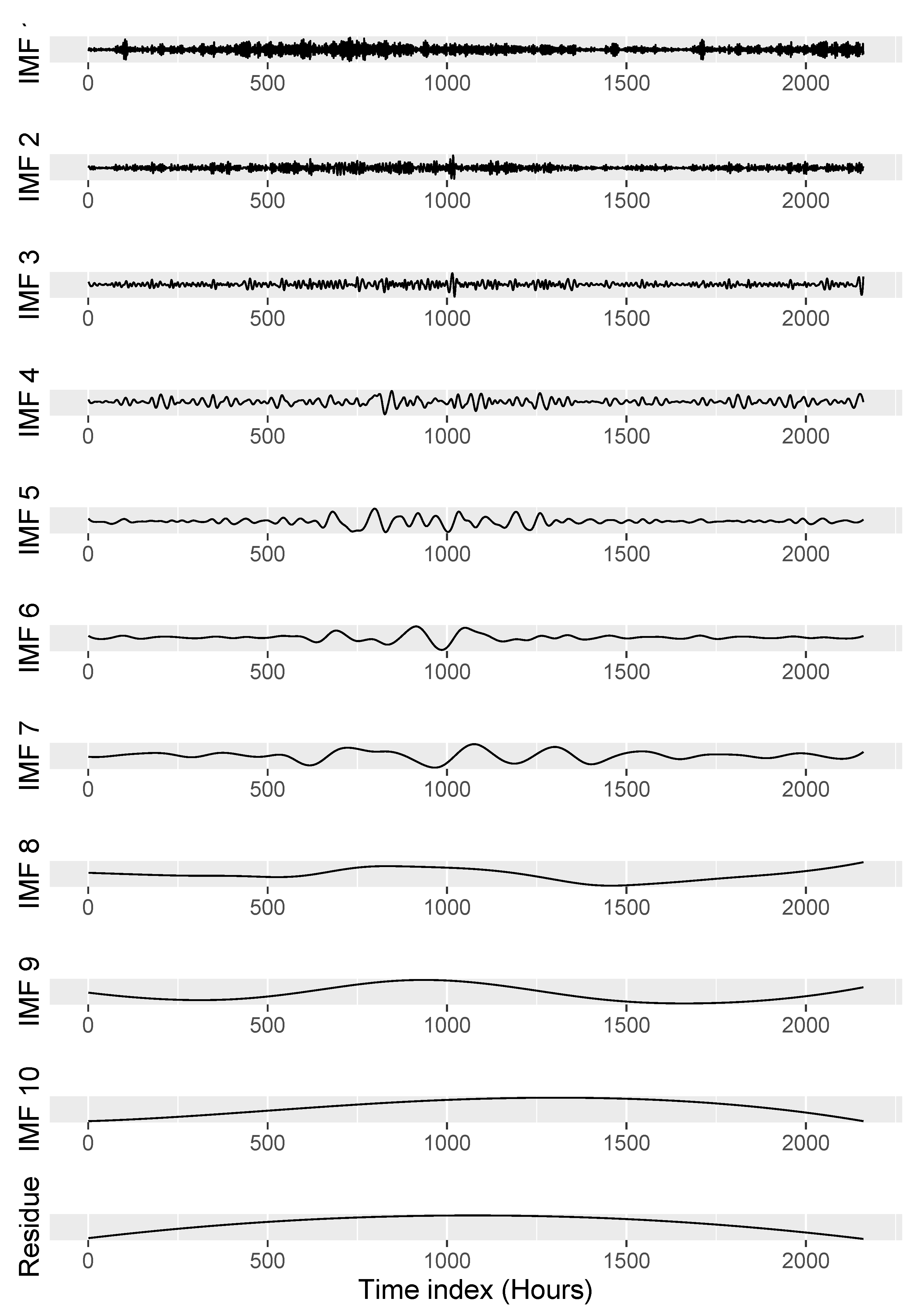
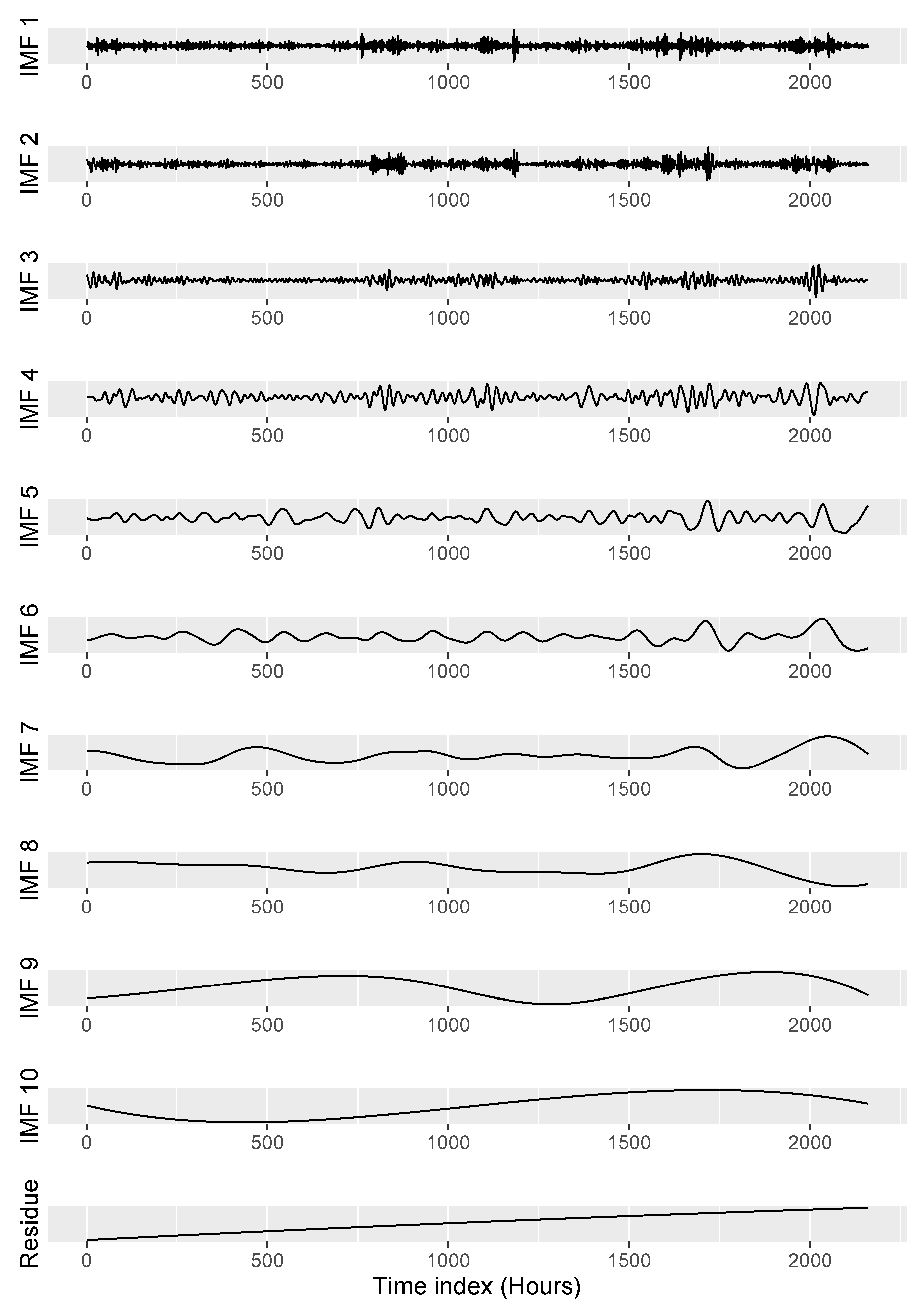
2.1. Empirical Mode Decomposition (EMD) Method

EMD is a very famous and widely accepted decomposition method that is generally applied to non-stationary and nonlinear time-series [28]. It decomposes such a time-series into a finite number of intrinsic modes known as IMFs and a residual.

This process is dependent only on the statistical nature of the time-series. Firstly, it finds local minimas and maximas in the time-series and generates lower and upper envelopes corresponding to the minima and maxima values, respectively, by using an interpolation method. Then, the average of lower and upper envelopes are removed from the original time-series to achieve the local IMFs. This procedure is repeated till following two situations get contented:

• mean of both envelopes (lower and upper) approaches zero
• count of minima and maxima, and zero crossings differs at most by one

This is a sifting process and represented as shown in (1).

$$x\left(t\right)=\sum _{i=1}^{N}IM{F}_i\left(t\right)+R_N\left(t\right)$$

(1)

where $IM{F}_i\left(t\right)$ and $R_N\left(t\right)$ represent generated IMFs and a residue with the decomposition method.

2.2. Ensemble Empirical Mode Decomposition (EEMD) Method

The conventional EMD usually suffers from the problem of mode mixing, which is an existence of the signal frquencies with highly desperate scales seen in IMFs. Ref. [33,54] discussed the mode mixing concept in detail. This problem of mode mixing is reduced significantly with the EEMD method which is the inheritor of EMD discussed in [32]. In EEMD method, the ultimate IMF signals are estimated by averaging IMFs obtained with trials of new noises. In EEMD, each trail consisting decomposed signals along with a white noise having finite amplitudes. It is interesting to observe that EEMD acts as a self-adaptive filter [55,56].

The procedure of the EEMD method is initiated by introducing white noise to the original wind power/speed time-series. Then IMFs and residue are generated with the EMD method. These two steps are repeated with different white noises and the corresponding IMFs are obtained. This process is repeated for few finite numbers, which is also known as ensemble numbers.

The final IMF and a residue generated with the EEMD method is achieved as the IMFs and the residue means at each repetition. However, the original time-series will not be achieved with the addition of these IMFs and residue, but, the EEMD method was supported in [32,33,34,35] because of its better prediction performance and smoother IMFs. In all these IMFs, similar scaled frequencies are obtained. This phenomena is discussed more detailly in [33,54].

2.3. Pattern Sequence based Forecasting (PSF) Method

The PSF method was proposed in [47] and then its utility was explained in detail in [48]. The prediction with the PSF method is dependent on patterns occurred in a time-series. It consists of sub-processes such as data normalization, clustering, clustered data based forecasting and de-normalization, etc. The novelty of this method is that, it uses labels for the patterns present in the data, and not using the original one. With the normalization process, the redundancies present in the data can be eliminated. It is done by (2).

$$X_j\leftarrow \frac{Xj}{\frac{1}{N}{\sum }_{i=1}^N{X}_i}$$

(2)

where N is its size in units of time and $X_j$ is the jth value of every cycle in the time-series.

In the PSF algorithm, the patterns present in the data are replaced with labels and it is done with clustering methods. This method produces clusters by k-means clustering. The advantages of the k-means clustering technique is that it is easy to use and consumes very few calculation time, but it needs the prior information of the number of centers into which the data has to be clustered. Ref. [47] suggested the so-called Silhouette index in order to decide suitable numbers of cluster centers, whereas, [48] suggested three different indices, i.e., the Dunn index [57], the Silhouette index [58], and the Davies-Bouldin index [59].

The ‘best two among three’ policy is used to find the optimum clusters. It means that cluster size will be finalized with a number returned by more than one index. [49,60,61] suggested and used a single index, which leads to simplification of computation for the clustering process. Then, prediction procedure is executed labels series.

The prediction process with the PSF method consists of different steps including optimum window size selection, matching of pattern sequences, and estimations. The sequence of last W labels (Window), is searched within the label series. While doing so, if the window is not repeated at least once, in such cases, the sequence size is reduced by one unit. Again, this process continues until the window repeats itself in the sequence of labels. During window pattern searching in the labels, the labels seen very next to all matched sequence is stored and its mean is considered as the next predicted value.

Finally, de-normalization is used to replace the labels with an appropriate value in the dataset. The predicted value is attached to the original time-series and the entire procedure is repeated to get the next forecasted value. This allows the prediction of multiple future values. The PSF algorithm is operated until the desired outcomes are obtained.

The optimum window size (W) selection in a challenging task in the prediction process of PSF such that the prediction error can be kept minimum. The mathematical representation for the window size selections is the minimization of (3),

$$\sum _{tϵTs}∥\widehat{X}\left(t\right)-X\left(t\right)∥$$

(3)

where $X\left(t\right)$ is the original time-series at time t and $\widehat{X}\left(t\right)$ is the corresponding forecasted values. Practically, cross-validation is used to calculate the window size (W). The methodology of PSF method discussed in [48] is shown in Figure 1.

An R package for the PSF method is explained in [61]. This R package ‘PSF’ [62] automatically calculate various parameters related to PSF method and forecasts the time-series.

2.4. Autoregressive Integrated Moving Average (ARIMA) Method

It method consists of differencing, auto-regression and the moving average model [63]. To fit an ARIMA model, it is necessary that the data is stationary. If not, it is made stationary with differencing technique.

ARIAM method is the combined form of differences, autoregression and moving average methods that is represented as $ARIMA(p,d,q)$, where p is the order of the autoregression, d is the degree of differencing and q is the order of the moving average method. Generally, these parameters ($p,d,q$) are calculated with autocorrelation graphs, Akaike’s information criterion (AIC) and Schwartz Bayesian information criterion (BIC) tests. The linear equation to state the ARIMA method for a time varying time-series $Y_t$ is shown in (4),

$${(1-B)}^d{Y}_t=\mu +\frac{\theta \left(B\right)}{\varphi \left(B\right)}{\alpha }_t$$

(4)

$\theta$ and $\varphi$ represents autoregression and moving average methods applied to a backshift operator B and mean is represented as $\mu$.

3. Proposed Methods

As explained in the introduction, in this work two new methodologies have been developed to improve the results obtained by using the four methods described in Section 2. This section is devoted to explain in detail both proposed methodologies.

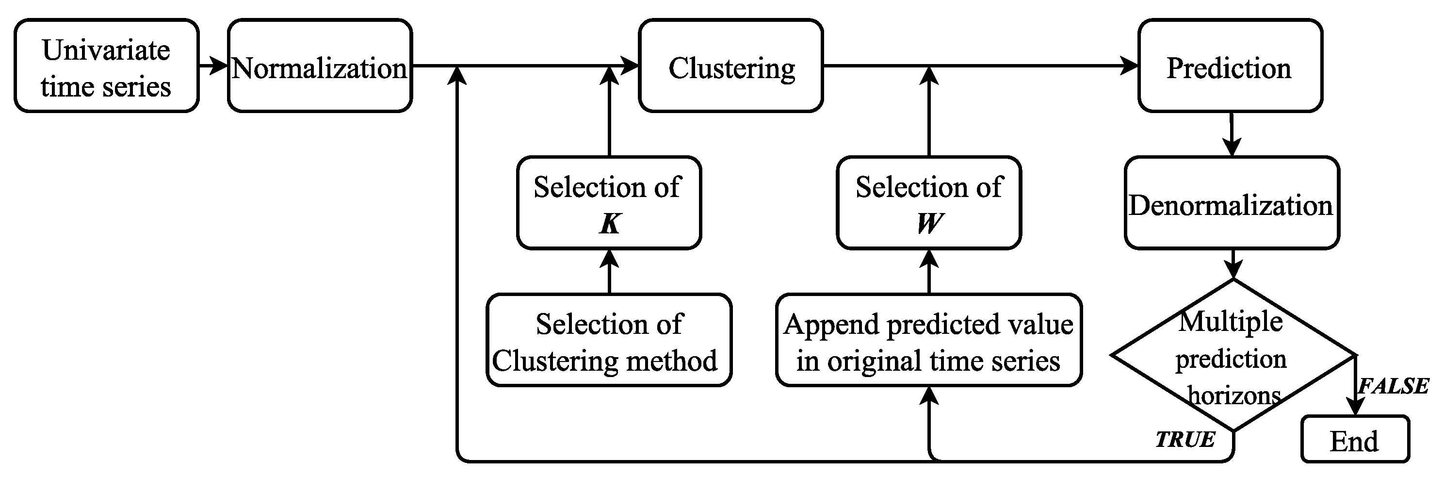
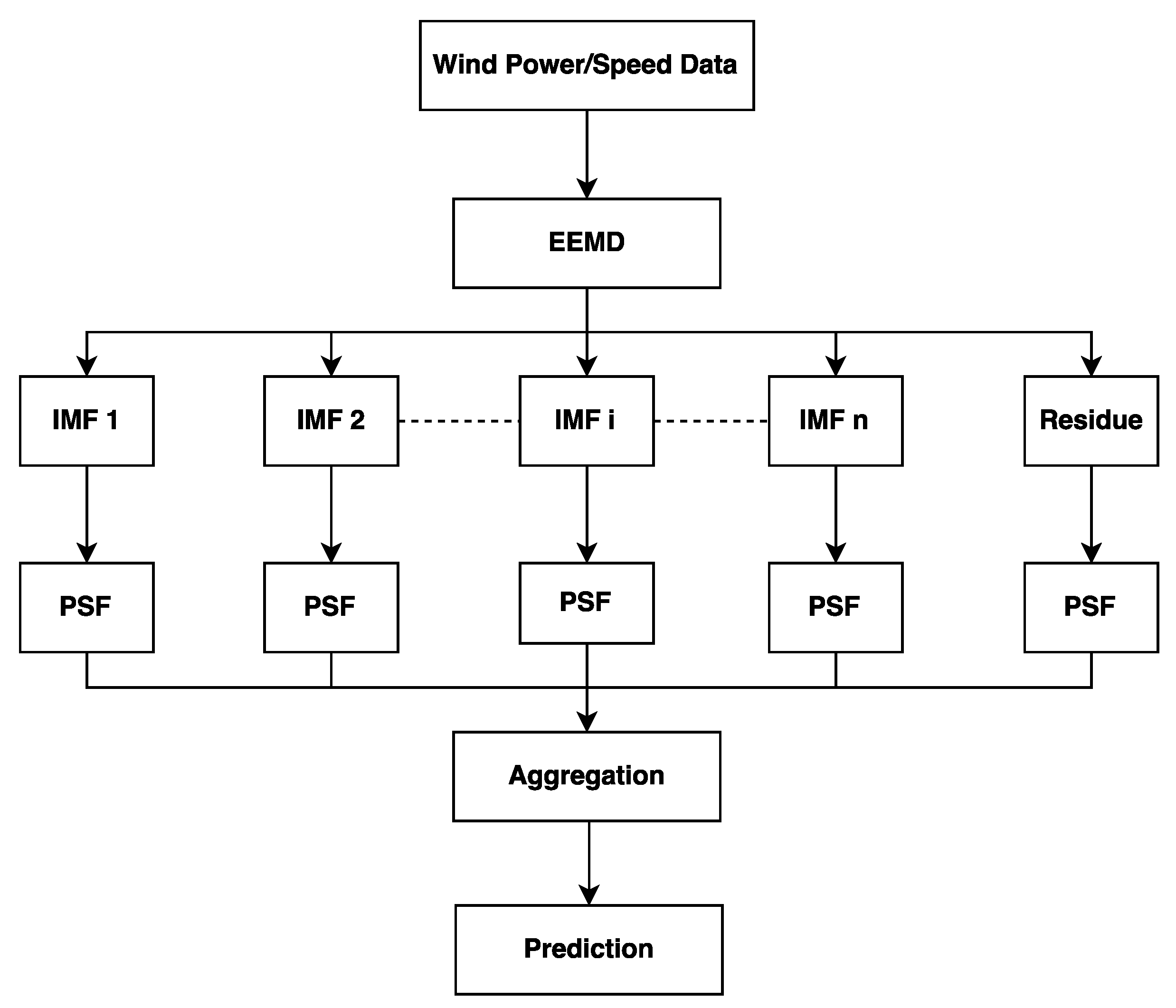
3.1. Hybrid EEMD-PSF Model

PSF is a useful method and proven successfully in time-series forecasting in various domains with satisfactory results [49,51,64]. Though the simple PSF method has many advantages over the conventional forecasting methods, it is tough task to forecast wind power or speed time-series accurately with it because of highly non-stationary and intermittent nature of such datasets. In order to overcome this inability of the PSF method, two new hybrid approaches are proposed in this paper. One of them consists of the hybridization of EEMD and PSF methods, denoted as Hybrid EEMD-PSF model. Whereas, the second one is denoted as hybrid EEMD-PSF-ARIMA model that is the hybridization of PSF, ARIMA and EEMD methods. This and next sections describe both proposed models in detail.

Most of the EMD based forecasting models follow a similar principle. Firstly, they decompose a time-series into sub-series and then forecast each sub-series with suitable methods. Secondly, the addition of all forecasted sub-series is noted as the final forecast result. A similar approach is used in the proposed hybrid model. All the sub-series (IMFs) are treated with the PSF method and the process of future value prediction is performed. The flowchart of the hybrid EEMD-PSF model is shown in Figure 2 and its corresponding procedure is explained as follows:

• Step 1: Apply EEMD method to transform a time-series in to a set of sub-series (IMFs and a residue).
• Step 2: Calculate the cluster size (K) and optimum window size (W) for the IMFs and residue.
• Step 3: Use PSF method to forecast all sub-series (IMFs and residue).
• Step 4: Add forecasted outcomes corresponding to all sub-series to achieve the ultimate forecasting results.

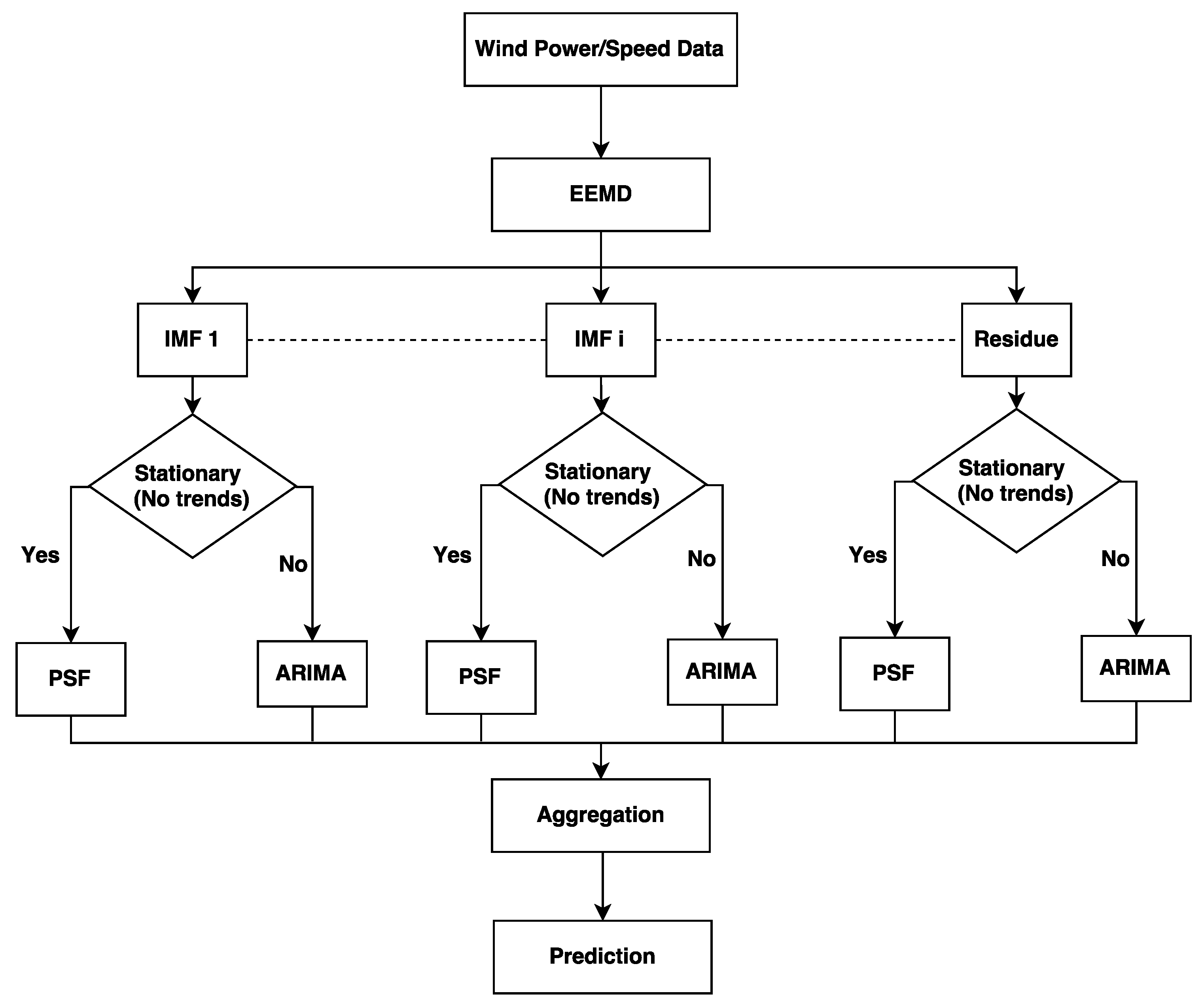
3.2. Hybrid EEMD-PSF-ARIMA Model

This is an extension of the EEMD-PSF model in association with the ARIMA method, which executes both PSF and ARIMA methods for prediction with the consideration of the time-series characteristics of respective IMFs and residue series. As discussed in upcoming sections, different IMFs exhibit distinct time-series characteristics (Refer Figures 5 and 7). Earlier few IMFs exhibit much higher frequencies and reflects the random and mainly noisy information present in wind power and wind speed time-series. Whereas, the middle range of IMFs are more periodic and looks with seasonal patterns as compared to earlier IMFs. Finally, the residue along with last few IMFs show trend components in the series. With the PSF method, it might be quite difficult to achieve accurate predictions for all types of IMFs with distinct types of time-series characteristics. There are many pieces of evidence [48,49,51,61] discussing the superior performance of PSF for stationary, seasonal and cyclic time-series, but it fails to achieve such accurate prediction in most of the cases with trendy and non-stationary time-series because of unavailability of pattern sequences in such trendy time-series. Whereas, methods such as ARIMA belonging to autoregression family achieve better prediction results for trendy and non-stationary time-series by introducing stationarity in such series.

In order to avail the advantages of autoregression based methods in the hybrid EEMD-PSF model, the non-stationary and trendy time-series are processed and predicted with the ARIMA method. This new model is named as hybrid EEMD-PSF-ARIMA model. The stationarity and trends characteristics of all IMFs and the residue are determined with the Kwiatkowski Phillips Schmidt Shin (KPSS) test [65]. This test uses a linear regression technique and breaks a time-series into three sections: (a) a deterministic trend, (b) a random walk, and (c) a stationary error. These sections are the deciding factors to understand the stationarity and trend nature of a time-series, statistically. This test finds out whether a time-series is stationary around a mean or a linear trend. The null hypothesis of KPSS test is that the data is trend stationary. This null hypothesis is rejected usually at 5% confidence level if the p-value associated with the test is lower than the significance level ($p-value<0.05$). With the inclusion of the KPSS test and the ARIMA method, the proposed hybrid EEMD-PSF-ARIMA method is modified as shown in the flowchart in Figure 3. The corresponding steps of EEMD-PSF-ARIMA are as follows:

• Step 1: Apply EEMD method to transform a time-series in to a set of sub-series (IMFs and a residue).
• Step 2: Execute the KPSS test on all IMFs and the residue to differentiate them in stationary and non-stationary groups.
• Step 3: Apply the PSF method on stationary IMFs and the ARIMA method on non-stationary IMFs.
• Step 4: Add forecasted outcomes corresponding to all sub-series to achieve the ultimate forecasting results.

4. Case Study

In this section, two case studies are discussed to evaluate the performance of the proposed methods. In the first one, they are examined on wind power time-series whereas in the second one, a wind speed time-series is used. In both cases, the short-term prediction is performed in two ways:

• 24 h-ahead prediction with iterated strategy, and
• multiple step ahead prediction with direct strategy (12 and 24 h).

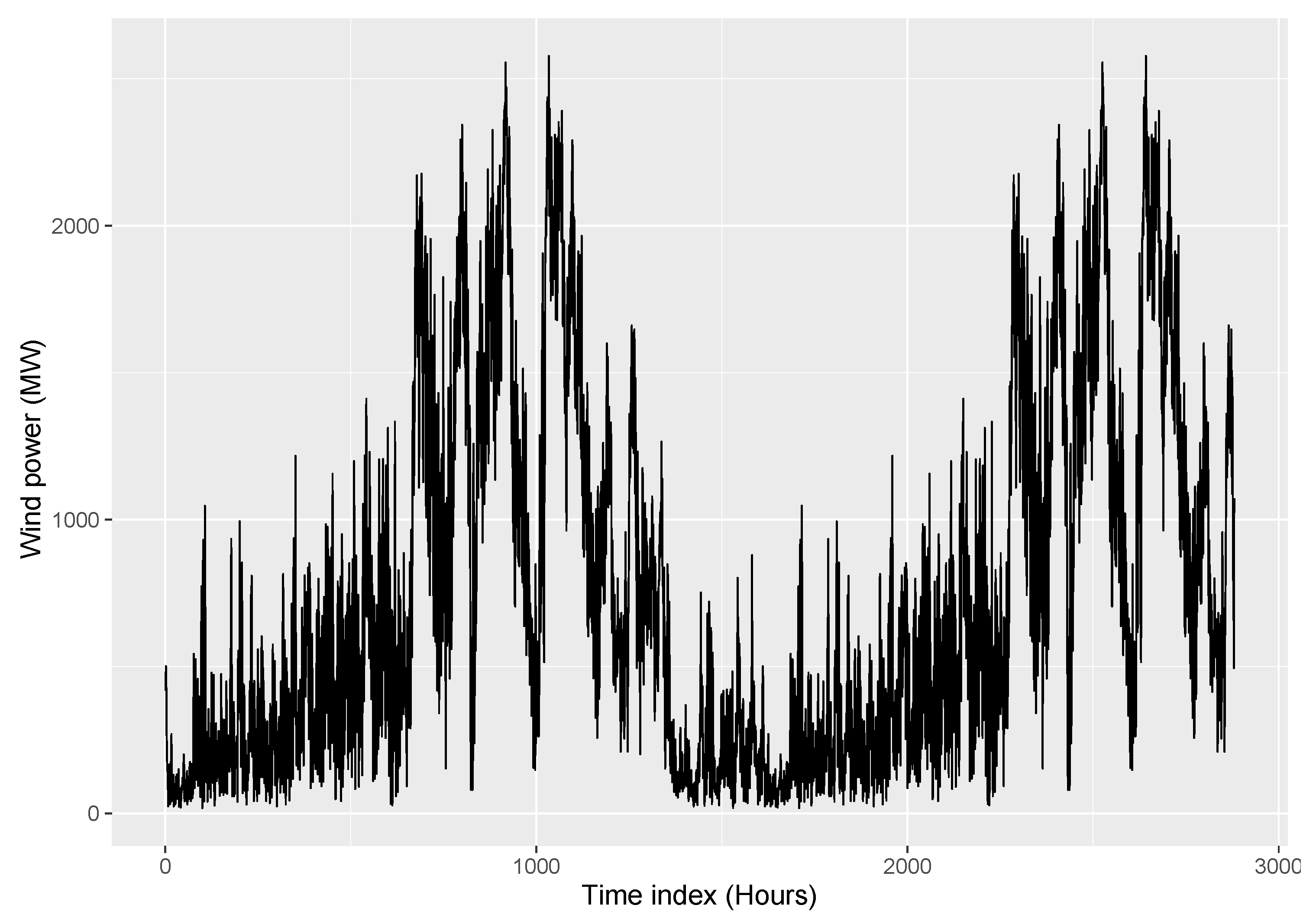
4.1. Case Study 1 - Wind Power Data

The wind power data used in this case study has been collected from an online Government portal which shows average hourly and daily generation of wind power in the state of Maharashtra, India. For this study, the data are taken from 1 January 2016 to 30 April 2016 and averaged over 1 h. No missing values were observed in data within this duration. The data within the first three months (January - March) are used for training and the remaining data are used for validation purpose. The hourly behavior of the wind power of this dataset is from 1 January 2016 to 31 March 2016 illustrated in Figure 4. Furthermore, the statistical parameters including mean, median and standard deviation are mentioned in

Table 1. Statistical details of wind power time-series.

Median	Mean	Maximum	Minimum	Standard Deviation
576.50	757.20	2578.0	18.0	623.53

.

To evaluate the prediction performance of the proposed methods, three error performance measures are used, i.e., Root mean square error (RMSE), Mean absolute error (MAE) and Mean absolute percentage error (MAPE). These error measures are defined in (5)–(7).

$$RMSE=\sqrt{\frac{1}{N}\sum _{i=1}^N{\left|X_i-{\widehat{X}}_i\right|}^2}$$

(5)

$$MAE=\frac{1}{N}\sum _{i=1}^N\left|X_i-{\widehat{X}}_i\right|$$

(6)

$$MAPE=\frac{1}{N}\sum _{i=1}^N\frac{\left|X_i-{\widehat{X}}_i\right|}{X_i}\times 100\%$$

(7)

where $X_i$ and ${\widehat{X}}_i$ original and the forecasted values, respectively. The RMSE and MAE describe the sample standard deviation and the average variance between the true value and the corresponding predicted values, respectively. Whereas, MAPE represents the sensitivity for minute change in the time-series. MAPE does not have any unit measure. Furthermore, the computation time is considered as one of the metrics for comparison of various prediction methods examined in the study.

4.1.1. Simulation

This section describes the proposed models (EEMD-PSF and EEMD-PSF-ARIMA) applied to the wind power time-series. Both of these models initiate with the decomposition of time-series into a finite number of IMFs and a residue with the EEMD technique. For the original series of mean hourly wind power data, 10 IMFs along with a residue are generated (Figure 5).

In the EEMD-PSF model, all sub-series (IMFs and a residue) are forecasted using PSF methodology. First of all, suitable values of clusters and window size are calculated for all IMFs, shown in

Table 2. Prediction method selection for IMFs in EEMD-PSF and EEMD-PSF-ARIMA model for wind power time-series.

IMFs	$\mathit{p}-\mathit{Value}$	EEMD-PSF (Method Selection)		EEMD-PSF-ARIMA (Method Selection)
IMF1	>0.05	PSF	(K = 3, W = 3)	PSF	(K = 3, W = 3)
IMF2	>0.05	PSF	(K = 3, W = 9)	PSF	(K = 3, W = 9)
IMF3	>0.05	PSF	(K = 3, W = 7)	PSF	(K = 3, W = 7)
IMF4	>0.05	PSF	(K = 3, W = 1)	PSF	(K = 3, W = 1)
IMF5	>0.05	PSF	(K = 3, W = 1)	PSF	(K = 3, W = 1)
IMF6	>0.05	PSF	(K = 2, W = 7)	PSF	(K = 2, W = 7)
IMF7	>0.05	PSF	(K = 4, W = 9)	PSF	(K = 4, W = 9)
IMF8	<0.05	PSF	(K = 3, W = 10)	ARIMA	(p = 1, d = 2, q = 0)
IMF9	<0.05	PSF	(K = 2, W = 1)	ARIMA	(p = 1, d = 2, q = 0)
IMF10	<0.05	PSF	(K = 2, W = 10)	ARIMA	(p = 0, d = 2, q = 5)
Residue	<0.05	PSF	(K = 2, W = 1)	ARIMA	(p = 0, d = 2, q = 0)

. With respect to these parameters, different PSF models are assigned for distinct IMFs and finally, the future values predicted for the desired duration. The aggregation of these predicted values corresponding to all IMFs series is treated as the prediction with EEMD-PSF model.

Conversely, the finite number of IMFs are differentiated into two clusters (stationary and non-stationary) in the EEMD-PSF-ARIMA model. The clustering of these IMFs is performed with the KPSS test, which follows the null hypothesis of time-series being stationary. The IMF series with p-values lower than 0.05 belonged to the non-stationary cluster and other IMFs were kept in the stationary one. All stationary signals without trendy characteristics are processed with the PSF method and trendy, non-stationary signals are processed with the ARIMA method. The corresponding optimum window and cluster size for the PSF method and $p,d,q$ parameters for the ARIMA method for respective IMFs and residue are shown in Table 2. Finally, the accumulation of all predicted values is considered as a final prediction with the EEMD-PSF-ARIMA model.

In this study, for evaluation of the proposed methods, forecasted results are compared with PSF, ARIMA and their hybrid combination models (EMD-PSF, EMD-ARIMA, EEMD-ARIMA, EMD-PSF-ARIMA). Furthermore, the benchmarked LSSVM and EEMD-LSSVM models generally used for wind power and wind speed prediction are compared in the study.

4.1.2. Comparison and Discussion

In this subsection, a performance of both proposed models is compared with various models including distinct combinations of PSF, ARIMA, EMD, and EEMD. Further, a comparative analysis is performed with LSSVM and EEMD-LSSVM models. To prove the superiority of the proposed models, different forecast techniques and horizons are selected. Prediction performance is examined on two different techniques of predictions, i.e., a) iterated strategy and b) direct strategy of prediction [66]. In iterated strategy approach, the prediction model predicts a small horizon value and uses this value along with the input time-series to predict the following forecast. Whereas, in the direct strategy approach, a model forecasts using only its observations in a single iteration. In [67], authors explained the difference between these strategies in this way: “Iterated multi-period ahead time-series forecasts are made using a one-period ahead model, iterated forward for the desired number of periods, whereas direct forecasts are made using a horizon-specific estimated model.”

In the iterated strategy, two cases are considered for comparison, i.e., one and two step ahead forecast. In the one step ahead iterated approach, for a given time-series, a very next value is predicted and this value is further considered for the prediction of the next value. While in the two step ahead iterated approach, two future values are predicted and these values are used for the prediction of the next two values.

To evaluate the performance of the proposed models, eight forecasting models are tested: PSF, ARIMA, LSSVM, hybrid models (EMD-PSF, EMD-ARIMA, EMD-LSSVM, EMD-PSF-ARIMA). One and two step ahead (iterated approach) predictions are carried out on all the models and future values are predicted for the next 24 h.

Table 3. Comparison of proposed methods with reported methods on RMSE, MAE and MAPE for one and two step ahead (iterate strategy) forecasting with wind power time-series.

Error Measures	RMSE		MAE		MAPE
Models	1 Step ahead	2 Steps ahead	1 Step ahead	2 Steps ahead	1 Step ahead	2 Steps ahead
EEMD-PSF-ARIMA	30.18	117.84	25.06	117.43	6.34	17.73
EEMD-PSF	49.95	147.89	44.24	133.19	8.27	17.93
EMD-PSF-ARIMA	98.64	175.67	92.41	143.95	16.33	22.02
EMD-PSF	148.14	182.69	135.88	170.64	24.83	28.38
PSF	174.73	185.21	169.02	175.43	26.92	28.91
EEMD-ARIMA	178.22	193.05	174.66	180.52	27.11	29.39
EMD-ARIMA	189.12	212.91	180.82	203.66	29.31	31.48
ARIMA	195.21	257.8	193.13	220.98	41.98	48.82
EEMD-LSSVM	202.07	262.37	197.08	245.06	43.78	50.43
LSSVM	226.92	262.76	221.28	258.31	47.28	52.27

shows the estimated errors in prediction in terms of RMSE, MAE, and MAPE measures. Similarly, a multiple-step ahead (direct strategy) forecast for the horizon of 12 and 24 h are shown in

Table 4. Comparison of proposed methods with reported methods on RMSE, MAE and MAPE for horizon prediction (direct strategy) of 12 and 24 h with wind power time-series.

Horizon	12 Hours			24 Hours
Models	RMSE	MAE	MAPE	RMSE	MAE	MAPE
EEMD-PSF-ARIMA	149.78	132.93	24.97	166.33	148.25	34.34
EEMD-PSF	152.29	137.56	25.73	184.88	167.06	38.40
EMS-PSF,ARIMA	185.8	157.48	29.3	216.96	189.85	46.72
EMD-PSF	200.24	179.46	38.96	226.78	203.34	51.97
PSF	205.54	191.94	39.85	241.88	217.16	57.59
EEMD-ARIMA	299.73	213.26	54.30	317.81	282.22	62.02
EMD-ARIMA	354.78	305.19	57.34	385.79	330.14	66.14
ARIMA	419.65	380.26	59.10	449.83	423.78	71.94
EEMD-LSSVM	434.60	406.22	60.52	482.54	436.06	74.54
LSSVM	460.03	422.01	65.46	517.57	473.97	78.76

with the same error measurements (RMSE, MAE, and MAPE).

From Table 3 and Table 4, the following conclusions can be extracted:

Compared with all models studied in the paper, the proposed models (EEMD-PSF and EEMD-PSF-ARIMA) are showing lower error values (for all error measures) in all cases, whether it is an iterated strategy or a direct strategy of prediction. For example, RMSE, MAE and MAPE values for EEMD-PSF-ARIMA are 30.18, 25.06 and 6.34% for one step ahead forecasts and it is 117.84, 117.43 and 17.73% for two step ahead forecasts. These error values were found to be minimum in the comparison table (refer Table 3). The EEMD-PSF comes out to be a second best model for the same approach to prediction.

A similar performance can be seen in a case of multiple-step ahead (direct strategy) forecast for both horizons (12 and 24 h). The minimum error values are observed for the EEMD-PSF-ARIMA model with respect to all three error measures (RMSE, MAE, and MAPE); the corresponding values are found to be 149.78, 132.93, and 24.97% for 12 h horizon and 166.33, 148.25 and 34.34% for 24 h horizon. Here also, EEMD-PSF performed comparable and ranked as second best in the comparison table (refer Table 4).

From Table 3 and Table 4, it can be seen that both proposed models straightaway outperformed all other models compared in the study. Usually, error measurements are considered as a primary measure to evaluate a performance of a prediction model, but as computation time should be one of the important concerns while evaluating the same,

Table 5. Comparison of computation time (in Seconds).

Models	Wind Power Data	Wind Speed Data
EMD-PSF-ARIMA	9.28	10.18
EEMD-PSF-ARIMA	8.48	10.95
EMD-PSF	7.10	9.75
EEMD-PSF	6.91	11.41
EMD-ARIMA	12.57	13.37
EEMD-ARIMA	10.37	7.2
PSF	1.35	1.68
ARIMA	0.49	0.48
LSSVM	1.11	0.26
EEMD-LSSVM	1.99	1.09

shows the computation time for all the models for 24 step ahead prediction (direct strategy).

The computation time for the proposed models is a bit greater than the one for models without decomposition techniques and its EMD combination counterparts, too. For 24 h horizon prediction (a direct strategy), EEMD-PSF-ARIMA consumed 8.48 s and EEMD-PSF consumed 6.91 s. Whereas, EMD-PSF-ARIMA, EMD-PSF, PSF and ARIMA models consume 9.28, 7.10, 1.35 and 0.49 s, respectively, as shown in Table 5. In other words, it can be said that the proposed methods are forecasting accurately at the cost of consumption of slightly more computation delays. Another interesting thing can be observed from Table 5. While comparing computation time for the PSF model (1.35 s) with that of its hybrid EMD-PSF model, this time increased up to 7.10 s. For sure, this delay is introduced because of the decomposition process and individual prediction processes for each IMFs and the residue. For the wind power time-series, the average computation time for EMD and EEMD decomposition methods are found to be 0.01 and 1.10 s, respectively. Even though the EEMD method consumes more computation time, its hybrid models with PSF, ARIMA, and PSF-ARIMA are consuming significantly less computation time as compared to that of EMD hybrid models (refer Table 5). There can be various reasons for this fact, but the most suitable reason can be the similar scaled nature of IMFs in the EEMD method as compared to the IMFs of the EMD method showing mode mixing problem. Both PSF and ARIMA methods might have forecasted IMFs within specific frequency range more quickly than the IMFs with a combination of multiple frequencies.

There are a large number of evidences (discussed in Section 1) which state, with the hybridization of a time-series prediction algorithm with EMD or EEMD methods, the prediction accuracy is improved by many folds. Similar results are observed in this study. If the prediction results with PSF models are compared with hybrid EMD-PSF model, the error (in terms of RMSE) is reduced by 6.24% and with EEMD-PSF model, it decreases by 15.29% for 24 h horizon prediction with a direct strategy (refer Table 4). Similar behavior of error is observed for ARIMA and its hybrid models (Table 4).

Finally,

Table 6. One-way ANOVA test (p-values) with respect to EEMD-PSF-ARIMA model.

Models	Wind Power Data	Wind Speed Data
EMD-PSF-ARIMA	1.13 $\times {10}^{-4}$	3.01 $\times {10}^{-7}$
EMD-PSF	2.53 $\times {10}^{-8}$	0.003
EEMD-PSF	1.29 $\times {10}^{-13}$	1.41 $\times {10}^{-9}$
EMD-ARIMA	0.087	4.4 $\times {10}^{-4}$
EEMD-ARIMA	0.009	0.007
PSF	2.83 $\times {10}^{-5}$	7.9 $\times {10}^{-4}$
ARIMA	0.043	5.46 $\times {10}^{-9}$
LSSVM	0.062	4.69 $\times {10}^{-7}$
EEMD-LSSVM	0.062	4.55 $\times {10}^{-7}$

illustrates the validation of the proposed hybrid EEMD-PSF-ARIMA model with an ANalysis Of VAriance (ANOVA) test [68,69]. It is used to compare the means of two or more samples based on assumptions of normality from the F distribution. The evaluation of the null hypothesis, which samples in two or more groups and they are selected from same mean values populations can be done with ANOVA test. It compared the results from the models selected for comparison. This test provided confirmation that the prediction results had different statistical behavior and improvements in precision between methods were meaningful statistically. In all comparisons, the one sided p-values were significant at $\alpha =0.05$, which suggests that the selection of the methods was appropriate and the proposed model can improve the prediction in most cases.

4.2. Case Study 2—Wind Speed Data

In this Section, the proposed models are examined on wind speed time-series. The wind speed time-series in this study has been collected in Galicia, which is an autonomous community located in North-Western Spain. The mean wind speed values are sampled every 10 min at several measure stations of the Galician meteorological network. These time-series correspond to four consecutive months as shown in Figure 6. The data corresponding to the initial three months are used for training purpose and the performance of prediction models are validated on the last month data. This time-series shows statistical characteristics (including mean and standard deviation) as noted in

Table 7. Statistical details of wind speed time-series.

Median	Mean	Maximum	Minimum	Standard Deviation
4.66	5.19	18.34	0.00	2.88

.

In case 2, the same performance measures are adopted as that of Case study 1, which includes RMSE, MAE, and MAPE along with a respective comparison with ANOVA test. Furthermore, the computation time is considered as another parameter for comparison.

4.2.1. Simulation

A wind speed time-series is studied, while the case 1 was focused on wind power data. A similar comparison background is maintained in case 2 and a similar length of time-series horizon is maintained for testing and validation of the proposed methods with similar error performance metrics. Various prediction models were examined such as in case 1. Both proposed models (EEMD-PSF and EEMD-PSF-ARIMA) initiate with the decomposition of wind speed time-series in to a set of sub-series (IMFs and a residue). For the given wind speed time-series, 10 true IMFs and a residue are observed as illustrated in Figure 7.

For the EEMD-PSF model, optimum window and cluster size parameters for all IMFs and the residue are estimated as shown in

Table 8. Prediction method selection for IMFs in EEMD-PSF and EEMD-PSF-ARIMA models for wind speed time-series.

IMFs	p-Value	EEMD-PSF (Method Selection)		EEMD-PSF-ARIMA (Method Selection)
IMF1	>0.05	PSF	(K = 6, W = 1)	PSF	(K = 6, W = 1)
IMF2	>0.05	PSF	(K = 10, W = 5)	PSF	(K = 10, W = 5)
IMF3	>0.05	PSF	(K = 4, W = 10)	PSF	(K = 4, W = 10)
IMF4	>0.05	PSF	(K = 3, W = 10)	PSF	(K = 3, W = 10)
IMF5	>0.05	PSF	(K = 6, W = 10)	PSF	(K = 6, W = 10)
IMF6	>0.05	PSF	(K = 4, W = 10)	PSF	(K = 4, W = 10)
IMF7	<0.05	PSF	(K = 4, W = 3)	ARIMA	(p = 1, d = 1, q = 0)
IMF8	<0.05	PSF	(K = 4, W = 1)	ARIMA	(p = 1, d = 2, q = 0)
IMF9	<0.05	PSF	(K = 2, W = 1)	ARIMA	(p = 1, d = 2, q = 0)
IMF10	<0.05	PSF	(K = 2, W = 1)	ARIMA	(p = 0, d = 2, q = 2)
Residue	<0.05	PSF	(K = 2, W = 10)	ARIMA	(p = 0, d = 2, q = 5)

. Whereas in the EEMD-PSF-ARIMA model, with the implementation of KPSS tests, all IMFs and the residue are classified among stationary and non-stationary clusters. Table 8 shows the optimum window and cluster size for stationary and non-trendy IMFs and ($p,d,q$) parameters for non-stationary and trendy IMFs. With these parameters, respective prediction methods (either PSF or ARIMA) are applied and future values are predicted. The aggregation of these values is noted as prediction results with the EEMD-PSF-ARIMA model.

In case 2 (similar to case 1), all contemporary methods are compared with the proposed ones and the comparison results are discussed in next section.

4.2.2. Comparison and Discussion

This section presents a brief description of the proposed hybrid models (EEMD-PSF and EEMD-PSF-ARIMA) for wind speed time-series prediction, similar to the case of wind power prediction discussed in case 1. To examine the usability and stability of the proposed methods on wind speed data, the same analysis techniques and tests are operated in case 2.

In order to avoid redundancy and achieve simplicity, only the evaluations are given in this subsection.

Table 9. Comparison of proposed methods with reported methods on RMSE, MAE and MAPE for one and two step ahead (iterate strategy) forecasting with wind speed time-series.

Error Measures	RMSE		MAE		MAPE
Models	1 Step Ahead	2 Steps Ahead	1 Step Ahead	2 Steps Ahead	1 Step Ahead	2 Steps Ahead
EEMD-PSF-ARIMA	0.15	0.18	0.13	0.16	4.2	6.17
EEMD-PSF	0.16	0.21	0.14	0.19	4.44	7.86
PSF	0.21	0.28	0.19	0.22	6.26	8.74
EMD-PSF-ARIMA	0.23	0.49	0.21	0.43	6.31	12.88
EEMD-ARIMA	0.23	0.47	0.21	0.32	6.29	12.07
EMD-PSF	0.47	0.71	0.39	0.63	12.78	15.18
EMD-ARIMA	0.23	0.61	0.21	0.57	6.36	13.49
EEMD-LSSVM	0.63	0.86	0.52	0.79	18.49	19.49
ARIMA	0.58	0.74	0.50	0.69	15.69	18.16
LSSVM	0.72	1.07	0.77	0.94	23.01	26.74

and

Table 10. Comparison of the proposed methods with the reported methods on RMSE, MAE and MAPE for horizon prediction (direct strategy) of 12 and 24 h with wind speed time-series.

Horizon	12 Hours			24 Hours
Models	RMSE	MAE	MAPE	RMSE	MAE	MAPE
EEMD-PSF-ARIMA	0.23	0.19	5.48	0.33	0.28	9.42
EEMD-PSF	0.34	0.28	8.18	0.36	0.29	11.14
PSF	0.42	0.38	11.03	0.45	0.34	15.01
EMD-PSF-ARIMA	0.66	0.58	16.61	0.84	0.76	21.88
EEMD-ARIMA	0.61	0.57	15.98	0.66	0.52	19.39
EMD-PSF	1.12	0.97	26.74	1.38	1.25	34.13
EMD-ARIMA	0.69	0.65	18.32	1.00	0.92	26.57
EEMD-LSSVM	1.20	1.10	29.37	1.61	1.42	39.42
ARIMA	1.17	1.00	27.72	1.46	1.41	38.47
LSSVM	1.48	1.47	31.21	1.73	1.45	39.44

show the prediction results for both proposed models with various prediction environments considering iterated and direct prediction strategies, respectively. In the iterated strategy, one and two steps forecast methods are used for 24 h ($24\times 6=144$ instances, since time-series is sampled at 10 min interval) horizon prediction. While in the direct strategy, data for 12 and 24 h are predicted and error measures are compared in Table 10. Furthermore, the computation time comparison for all models under study is noted in Table 5. Finally, forecasted outcomes of the proposed model EEMD-PSF-ARIMA is validated with an ANOVA test with the corresponding statistical significance shown in Table 6.

The observation in Table 3, Table 4, Table 9 and Table 10 indicates that hybridization of PSF and EEMD methods has improved the prediction accuracy and further predicting stationary IMF series with PSF and remaining IMFs with ARIMA significantly improved the overall performance of the hybrid EEMD-PSF-ARIMA method in both direct and iterated approaches. Furthermore, it can be seen that the main results are similar to wind power data in case 1, such as:

• Prediction with the proposed models (EEMD-PSF and EEMD-PSF-ARIMA) is more accurate as compared to other methods.
• The hybridization with EMD and EEMD methods with PSF, ARIMA, and LSSVM methods lead to more accurate predictions as compared to their original forms.
• Similar to case 1, the trade-off between accuracy in prediction and computation time consumption is observed in case 2. For example, EEMD-ARIMA and EMD-ARIMA show more prediction accuracy at the cost of excess in computation delays.
• While discussing computation time, there are a few different things from case 1:

  (a)

  the performance of the PSF model is better than that of the EMD-PSF model in terms of prediction accuracy as well as computation time, and

  (b)

  the computation time for models hybridized with the EEMD method noted longer than the models hybridized with the EMD method. For example, the EEMD-PSF consumed 11.41 s, whereas the EMD-PSF completed the task in 9.75 s.

• In Table 6, the ANOVA test results are shown. The EEMD-PSF-ARIMA model prediction results show one-sided p-values significant at $\alpha =0.05$ and show statistical significance of the proposed comparison.

5. Conclusions

Accurate modeling of wind power/speed is an essential process for securing a reliable and clean energy production. An energy dispatch center uses real wind power and wind speed data to carry out unit commitment to the energy traders. Hence, the energy scheduling and economic dispatch plays an important role in such business models which are directly dependent on the accurate forecast of wind power and speed data. In this paper, two hybrid prediction methods named EEMD-PSF and EEMD-PSF-ARIMA are developed to enhance the forecasting accuracy in both wind power and speed time-series modeling. The EEMD-PSF model is the hybridization of PSF and EEMD methods; whereas, the EEMD-PSF-ARIMA model is the conditional hybridization version of EEMD, PSF and ARIMA methods. In both models, the EEMD method is used to decompose the original wind speed or power series into a finite number of sub-series and the forecasting of each sub-series was established by respective prediction methods. In the EEMD-PSF model, all sub-series were predicted with the PSF method. On the other hand; the EEMD-PSF-ARIMA model, the sub-series with high and low frequencies were predicted using PSF and ARIMA, respectively. The selection of PSF or ARIMA methods for the prediction process was dependent on the time-series characteristics of the decomposed series obtained with EEMD method. The KPSS test was used to characterize the sub-series into stationary and non-stationary subsets. In the EEMD-PSF-ARIMA model, stationary series were processed with the PSF method, while remaining series were processed with the ARIMA method.

Both proposed models were evaluated and assessed with iterated and direct strategy of prediction for the targeted forecasting value of the next 24 h. Different statistical indicators such as RMSE, MAE, MAPE and computation time were performed for the results evaluation. In all prediction environments, the EEMD-PSF-ARIMA model outperformed all the other methods; whereas, the EEMD-PSF secured the second best position. Simulations reveal that both methods have the following advantages (All quantitative comparisons presented here are on the basis of the RMSE metric.):

• In case of short-term wind power time-series prediction, both proposed methods have shown at least 18.03 and 14.78 percentage improvement in forecast accuracy as compared to contemporary methods considered in this study for direct and iterated strategies, respectively. Similarly, for wind speed data, those improvement observed to be 20.00 and 23.80 percentages, respectively.
• In all cases, EEMD-PSF-ARIMA has outperformed in terms of prediction accuracy improvements by at least 10.03 and 8.33 percentages in wind power and speed data, respectively. In wind power data, this achievement is attained at the cost of minute computation delay in the EEMD-PSF-ARIMA model better than EEMD-PSF model by merely few seconds. Conversely, in wind time-series, the EEMD-PSF-ARIMA model takes lesser computation delay as compared to the EEMD-PSF model. Hence, it can be stated that the forecasting accuracy benefits are much greater than the harm produced by the time delay.
• Furthermore, the hybridization of a prediction method with the EEMD method has improved the prediction accuracy significantly. For example, in wind power time-series, EEMD-PSF, EEMD-ARIMA, and EEMD-LSSVM models have shown 23.56, 29.34 and 6.76 percentage improvements in prediction accuracy, better than simple PSF, ARIMA, and LSSVM models, respectively.

The results’ comparison indicates that ARIMA models succeed in predicting low-frequency components (IMFs) more accurately than PSF models, but the overall enhancement in the prediction accuracy was achieved with high-frequency components prediction using PSF models as can be observed by the comparison of EEMD-PSF and EEMD-PSF-ARIMA model prediction results with that of EEMD-ARIMA model. In addition, the relation between the prediction error and computation time for the models hybridized with EMD and EEMD are discussed, which shows improvement in forecasting results at the cost of computation delays. In future, the computational delay can be reduced by aggregating IMFs with similar characteristics and reducing the number of models than used in the present study. Finally, the significance of the proposed models are assured with an ANOVA test and the R package (decomposedPSF) for proposed models are discussed in Appendix A.

References

1. Kisi, O.; Heddam, S.; Yaseen, Z.M. The implementation of univariable scheme-based air temperature for solar radiation prediction: New development of dynamic evolving neural-fuzzy inference system model. Appl. Energy 2019, 241, 184–195. [Google Scholar] [CrossRef]
2. Maroufpoor, S.; Sanikhani, H.; Kisi, O.; Deo, R.C.; Yaseen, Z.M. Long-term modelling of wind speeds using six different heuristic artificial intelligence approaches. Int. J. Climatol. 2019, 39, 3543–3557. [Google Scholar] [CrossRef]
3. Yuan, X.; Chen, C.; Yuan, Y.; Huang, Y.; Tan, Q. Short-term wind power prediction based on LSSVM–GSA model. Energy Convers. Manag. 2015, 101, 393–401. [Google Scholar] [CrossRef]
4. Zhu, X.; Genton, M.G. Short-Term Wind Speed Forecasting for Power System Operations. Int. Stat. Rev. 2012, 80, 2–23. [Google Scholar] [CrossRef]
5. Bokde, N.D.; Feijóo, A.; Al-Ansari, N.; Yaseen, Z.M. A comparison between reconstruction methods for generation of synthetic time series applied to wind speed simulation. IEEE Access 2019, 7, 135386–135398. [Google Scholar] [CrossRef]
6. Erdem, E.; Shi, J. ARMA based approaches for forecasting the tuple of wind speed and direction. Appl. Energy 2011, 88, 1405–1414. [Google Scholar] [CrossRef]
7. Xu, Q.; He, D.; Zhang, N.; Kang, C.; Xia, Q.; Bai, J.; Huang, J. A short-term wind power forecasting approach with adjustment of numerical weather prediction input by data mining. IEEE Trans. Sustain. Energy 2015, 6, 1283–1291. [Google Scholar] [CrossRef]
8. Carvalho, D.; Rocha, A.; Gómez-Gesteira, M.; Santos, C. A sensitivity study of the WRF model in wind simulation for an area of high wind energy. Environ. Model. Softw. 2012, 33, 23–34. [Google Scholar] [CrossRef] [Green Version]
9. Treiber, N.A.; Heinermann, J.; Kramer, O. Wind Power Prediction with Machine Learning. In Computational Sustainability; Springer: Berlin/Heidelberg, Germany, 2016; pp. 13–29. [Google Scholar]
10. Bludszuweit, H.; Domínguez-Navarro, J.A.; Llombart, A. Statistical analysis of wind power forecast error. IEEE Trans. Power Syst. 2008, 23, 983–991. [Google Scholar] [CrossRef]
11. Zhou, J.; Shi, J.; Li, G. Fine tuning support vector machines for short-term wind speed forecasting. Energy Convers. Manag. 2011, 52, 1990–1998. [Google Scholar] [CrossRef]
12. Salcedo-Sanz, S.; Ortiz-Garcı, E.G.; Pérez-Bellido, Á.M.; Portilla-Figueras, A.; Prieto, L. Short term wind speed prediction based on evolutionary support vector regression algorithms. Expert Syst. Appl. 2011, 38, 4052–4057. [Google Scholar] [CrossRef]
13. Azad, H.B.; Mekhilef, S.; Ganapathy, V.G. Long-term wind speed forecasting and general pattern recognition using neural networks. IEEE Trans. Sustain. Energy 2014, 5, 546–553. [Google Scholar] [CrossRef]
14. Ata, R.; Çetin, N.S. Analysis of height affect on average wind speed by ANN. Math. Comput. Appl. 2011, 16, 556–564. [Google Scholar] [CrossRef] [Green Version]
15. Rajagopalan, S.; Santoso, S. Wind power forecasting and error analysis using the autoregressive moving average modeling. In Proceedings of the Power & Energy Society General Meeting, Calgary, AB, Canada, 26–30 July 2009; pp. 1–6. [Google Scholar]
16. Zhang, W.; Su, Z.; Zhang, H.; Zhao, Y.; Zhao, Z. Hybrid wind speed forecasting model study based on SSA and intelligent optimized algorithm. Abstr. Appl. Anal. 2014, 2014. [Google Scholar] [CrossRef]
17. Shi, J.; Ding, Z.; Lee, W.J.; Yang, Y.; Liu, Y.; Zhang, M. Hybrid forecasting model for very-short term wind power forecasting based on grey relational analysis and wind speed distribution features. IEEE Trans. Smart Grid 2014, 5, 521–526. [Google Scholar] [CrossRef]
18. Kavasseri, R.G.; Seetharaman, K. Day-ahead wind speed forecasting using f-ARIMA models. Renew. Energy 2009, 34, 1388–1393. [Google Scholar] [CrossRef]
19. Eymen, A.; Köylü, Ü. Seasonal trend analysis and ARIMA modeling of relative humidity and wind speed time series around Yamula Dam. Meteorol. Atmos. Phys. 2019, 131, 601–612. [Google Scholar] [CrossRef]
20. Cadenas, E.; Rivera, W. Wind speed forecasting in three different regions of Mexico, using a hybrid ARIMA–ANN model. Renew. Energy 2010, 35, 2732–2738. [Google Scholar] [CrossRef]
21. Liu, H.; Erdem, E.; Shi, J. Comprehensive evaluation of ARMA–GARCH (-M) approaches for modeling the mean and volatility of wind speed. Appl. Energy 2011, 88, 724–732. [Google Scholar] [CrossRef]
22. Liu, H.; Tian, H.Q.; Li, Y.F. Comparison of two new ARIMA-ANN and ARIMA-Kalman hybrid methods for wind speed prediction. Appl. Energy 2012, 98, 415–424. [Google Scholar] [CrossRef]
23. Cadenas, E.; Rivera, W.; Campos-Amezcua, R.; Heard, C. Wind speed prediction using a univariate ARIMA model and a multivariate NARX model. Energies 2016, 9, 109. [Google Scholar] [CrossRef] [Green Version]
24. Cai, H.; Jia, X.; Feng, J.; Yang, Q.; Hsu, Y.M.; Chen, Y.; Lee, J. A combined filtering strategy for short term and long term wind speed prediction with improved accuracy. Renew. Energy 2019, 136, 1082–1090. [Google Scholar] [CrossRef]
25. Yaseen, Z.M.; Mohtar, W.H.M.W.; Ameen, A.M.S.; Ebtehaj, I.; Razali, S.F.M.; Bonakdari, H.; Salih, S.Q.; Al-Ansari, N.; Shahid, S. Implementation of univariate paradigm for streamflow simulation using hybrid data-driven model: Case study in tropical region. IEEE Access 2019, 7, 74471–74481. [Google Scholar] [CrossRef]
26. Jiang, P.; Wang, Y.; Wang, J. Short-term wind speed forecasting using a hybrid model. Energy 2017, 119, 561–577. [Google Scholar] [CrossRef]
27. Taswell, C.; McGill, K.C. Algorithm 735: Wavelet transform algorithms for finite-duration discrete-time signals. ACM Trans. Math. Softw. (TOMS) 1994, 20, 398–412. [Google Scholar] [CrossRef]
28. Huang, N.E.; Shen, Z.; Long, S.R.; Wu, M.C.; Shih, H.H.; Zheng, Q.; Yen, N.C.; Tung, C.C.; Liu, H.H. The empirical mode decomposition and the Hilbert spectrum for nonlinear and non-stationary time series analysis. In Proceedings of the Royal Society of London A: Mathematical, Physical and Engineering Sciences; The Royal Society: London, UK, 1998; Volume 454, pp. 903–995. [Google Scholar]
29. Liu, H.; Chen, C.; Tian, H.q.; Li, Y.F. A hybrid model for wind speed prediction using empirical mode decomposition and artificial neural networks. Renew. Energy 2012, 48, 545–556. [Google Scholar] [CrossRef]
30. Ren, Y.; Suganthan, P.; Srikanth, N. A comparative study of empirical mode decomposition-based short-term wind speed forecasting methods. IEEE Trans. Sustain. Energy 2015, 6, 236–244. [Google Scholar] [CrossRef]
31. Ren, Y.; Suganthan, P.N.; Srikanth, N. A novel empirical mode decomposition with support vector regression for wind speed forecasting. IEEE Trans. Neural Netw. Learn. Syst. 2016, 27, 1793–1798. [Google Scholar] [CrossRef]
32. Wu, Z.; Huang, N.E. Ensemble empirical mode decomposition: A noise-assisted data analysis method. Adv. Adapt. Data Anal. 2009, 1, 1–41. [Google Scholar] [CrossRef]
33. Wang, S.; Zhang, N.; Wu, L.; Wang, Y. Wind speed forecasting based on the hybrid ensemble empirical mode decomposition and GA-BP neural network method. Renew. Energy 2016, 94, 629–636. [Google Scholar] [CrossRef]
34. Hu, J.; Wang, J.; Zeng, G. A hybrid forecasting approach applied to wind speed time series. Renew. Energy 2013, 60, 185–194. [Google Scholar] [CrossRef]
35. Yu, C.; Li, Y.; Zhang, M. Comparative study on three new hybrid models using Elman Neural Network and Empirical Mode Decomposition based technologies improved by Singular Spectrum Analysis for hour-ahead wind speed forecasting. Energy Convers. Manag. 2017, 147, 75–85. [Google Scholar] [CrossRef]
36. Bokde, N.; Feijóo, A.; Villanueva, D.; Kulat, K. A Review on Hybrid Empirical Mode Decomposition Models for Wind Speed and Wind Power Prediction. Energies 2019, 12, 254. [Google Scholar] [CrossRef] [Green Version]
37. Qin, Q.; Lai, X.; Zou, J. Direct Multistep Wind Speed Forecasting Using LSTM Neural Network Combining EEMD and Fuzzy Entropy. Appl. Sci. 2019, 9, 126. [Google Scholar] [CrossRef] [Green Version]
38. Wu, Q.; Lin, H. Short-term wind speed forecasting based on hybrid variational mode decomposition and least squares support vector machine optimized by bat algorithm model. Sustainability 2019, 11, 652. [Google Scholar] [CrossRef] [Green Version]
39. Lu, P.; Ye, L.; Sun, B.; Zhang, C.; Zhao, Y.; Teng, J. A new hybrid prediction method of ultra-short-term wind power forecasting based on EEMD-PE and LSSVM optimized by the GSA. Energies 2018, 11, 697. [Google Scholar] [CrossRef] [Green Version]
40. Santhosh, M.; Venkaiah, C.; Kumar, D.V. Ensemble empirical mode decomposition based adaptive wavelet neural network method for wind speed prediction. Energy Convers. Manag. 2018, 168, 482–493. [Google Scholar] [CrossRef]
41. Young, I.R.; Ribal, A. Multiplatform evaluation of global trends in wind speed and wave height. Science 2019, 364, 548–552. [Google Scholar] [CrossRef]
42. Hong, D.; Ji, T.; Zhang, L.; Li, M.; Wu, Q. An indirect short-term wind power forecast approach with multi-variable inputs. In Proceedings of the Innovative Smart Grid Technologies-Asia, Melbourne, VIC, Australia, 28 November–1 December 2016; pp. 793–798. [Google Scholar]
43. Sohoni, V.; Gupta, S.; Nema, R. A Critical Review on Wind Turbine Power Curve Modelling Techniques and Their Applications in Wind Based Energy Systems. J. Energy 2016, 2016. [Google Scholar] [CrossRef] [Green Version]
44. Tian, J.; Zhou, D.; Su, C.; Soltani, M.; Chen, Z.; Blaabjerg, F. Wind turbine power curve design for optimal power generation in wind farms considering wake effect. Energies 2017, 10, 395. [Google Scholar] [CrossRef] [Green Version]
45. Bokde, N.; Feijóo, A.; Villanueva, D. Wind Turbine Power Curves Based on the Weibull Cumulative Distribution Function. Appl. Sci. 2018, 8, 1757. [Google Scholar] [CrossRef] [Green Version]
46. Bokde, N.; Feijóo, A.; Villanueva, D.; Kulat, K. A Novel and Alternative Approach for Direct and Indirect Wind-Power Prediction Methods. Energies 2018, 11, 2923. [Google Scholar] [CrossRef] [Green Version]
47. Martínez-Álvarez, F.; Troncoso, A.; Riquelme, J.C.; Aguilar-Ruiz, J.S. LBF: A labeled-based forecasting algorithm and its application to electricity price time series. In Proceedings of the International Conference on Data Mining, Pisa, Italy, 15–19 December 2008; pp. 453–461. [Google Scholar]
48. Martínez-Álvarez, F.; Troncoso, A.; Riquelme, J.C.; Aguilar-Ruiz, J.S. Energy time series forecasting based on pattern sequence similarity. IEEE Trans. Knowl. Data Eng. 2011, 23, 1230–1243. [Google Scholar] [CrossRef]
49. Majidpour, M.; Qiu, C.; Chu, P.; Gadh, R.; Pota, H.R. Modified pattern sequence-based forecasting for electric vehicle charging stations. In Proceedings of the International Conference on Smart Grid Communications (SmartGridComm), Venice, Italy, 3–6 November 2014; pp. 710–715. [Google Scholar]
50. Koprinska, I.; Rana, M.; Troncoso, A.; Martínez-Álvarez, F. Combining pattern sequence similarity with neural networks for forecasting electricity demand time series. In Proceedings of the International Joint Conference on Neural Networks (IJCNN), Dallas, TX, USA, 4–9 August 2013; pp. 1–8. [Google Scholar]
51. Fujimoto, Y.; Hayashi, Y. Pattern sequence-based energy demand forecast using photovoltaic energy records. In Proceedings of the International Conference on Renewable Energy Research and Applications (ICRERA), Nagasaki, Japan, 11–14 November 2012; pp. 1–6. [Google Scholar]
52. Bokde, N.; Wakpanjar, A.; Kulat, K.; Feijoo, A.E. Robust performance of PSF method over outliers and random patterns in univariate time series forecasting. In Proceedings of the International Technology Congress, Pune, India, 28–29 December 2017. [Google Scholar]
53. Bokde, N.; Troncoso, A.; Asencio-Cortés, G.; Kulat, K.; Martínez-Álvarez, F. Pattern sequence similarity based techniques for wind speed forecasting. In International Work-Conference on Time Series; Universidad de Granada: Granada, Spain, 2017. [Google Scholar]
54. Wang, Y.; Wang, S.; Zhang, N. A novel wind speed forecasting method based on ensemble empirical mode decomposition and GA-BP neural network. In Proceedings of the Power and Energy Society General Meeting, Vancouver, BC, Canada, 21–25 July 2013; pp. 1–5. [Google Scholar]
55. Flandrin, P.; Rilling, G.; Goncalves, P. Empirical mode decomposition as a filter bank. IEEE Signal Process. Lett. 2004, 11, 112–114. [Google Scholar] [CrossRef] [Green Version]
56. Wu, Z.; Huang, N.E. A study of the characteristics of white noise using the empirical mode decomposition method. In Proceedings of the Royal Society of London A: Mathematical, Physical and Engineering Sciences; The Royal Society: London, UK, 2004; Volume 460, pp. 1597–1611. [Google Scholar]
57. Dunn, J.C. Well-separated clusters and optimal fuzzy partitions. J. Cybern. 1974, 4, 95–104. [Google Scholar] [CrossRef]
58. Kaufman, L.; Rousseeuw, P.J. Finding Groups in Data: An Introduction to Cluster Analysis; John Wiley & Sons: Hoboken, NJ, USA, 2009; Volume 344. [Google Scholar]
59. Davies, D.L.; Bouldin, D.W. A cluster separation measure. IEEE Trans. Pattern Anal. Mach. Intell. 1979, 2, 224–227. [Google Scholar] [CrossRef]
60. Jin, C.H.; Pok, G.; Park, H.W.; Ryu, K.H. Improved pattern sequence-based forecasting method for electricity load. IEEJ Trans. Electr. Electron. Eng. 2014, 9, 670–674. [Google Scholar] [CrossRef]
61. Bokde, N.; Asencio-Cortes, G.; Martinez-Alvarez, F.; Kulat, K. PSF: Introduction to R Package for Pattern Sequence Based Forecasting Algorithm. R J. 2017, 9, 324–333. [Google Scholar] [CrossRef] [Green Version]
62. Bokde, N.; Asencio-Cortes, G.; Martinez-Alvarez, F. PSF: Forecasting of Univariate Time Series Using the Pattern Sequence-Based Forecasting (PSF) Algorithm; R Package Version 0.4; 2017. [Google Scholar]
63. Box, G.; Jenkins, G. Some comments on a paper by Chatfield and Prothero and on a review by Kendall. J. R. Stat. Society. Ser. A (General) 1973, 136, 337–352. [Google Scholar] [CrossRef]
64. Bokde, N.; Feijóo, A.; Kulat, K. Analysis of differencing and decomposition preprocessing methods for wind speed prediction. Appl. Soft Comput. 2018, 71, 926–938. [Google Scholar] [CrossRef]
65. Kwiatkowski, D.; Phillips, P.C.; Schmidt, P.; Shin, Y. Testing the null hypothesis of stationarity against the alternative of a unit root: How sure are we that economic time series have a unit root? J. Econom. 1992, 54, 159–178. [Google Scholar] [CrossRef]
66. Bao, Y.; Xiong, T.; Hu, Z. Multi-step-ahead time series prediction using multiple-output support vector regression. Neurocomputing 2014, 129, 482–493. [Google Scholar] [CrossRef] [Green Version]
67. Marcellino, M.; Stock, J.H.; Watson, M.W. A comparison of direct and iterated multistep AR methods for forecasting macroeconomic time series. J. Econom. 2006, 135, 499–526. [Google Scholar] [CrossRef] [Green Version]
68. Armstrong, R.A.; Slade, S.; Eperjesi, F. An introduction to analysis of variance (ANOVA) with special reference to data from clinical experiments in optometry. Ophthalmic Physiol. Opt. 2000, 20, 235–241. [Google Scholar] [CrossRef] [PubMed]
69. Games, P.; Keselman, H.; Rogan, J. A review of simultaneous painvise multiple comparisons. Stat. Neerl. 1983, 37, 53–58. [Google Scholar] [CrossRef]
70. Bokde, N. decomposedPSF: Time Series Prediction with PSF and Decomposition Methods (EMD and EEMD); R Package Version 0.1.3; 2017. [Google Scholar]
Figure 1. PSF algorithm block diagram (Source: [46,61]).
Energies 13 01666 g001
Figure 2. The procedure of EEMD-PSF model.
Energies 13 01666 g002
Figure 3. The procedure of EEMD-PSF-ARIMA model.
Energies 13 01666 g003
Figure 4. Mean hourly Wind power time-series.
Energies 13 01666 g004
Figure 5. The decomposition of mean hourly Wind power time-series by EEMD method.
Energies 13 01666 g005
Figure 6. Mean wind speed time-series sampled at 10 min.
Energies 13 01666 g006
Figure 7. The decomposition of mean wind speed time-series (sampled at 10 min) by EEMD method.
Energies 13 01666 g007