Machine Learning Modeling of Horizontal Photovoltaics Using Weather and Location Data

 , ,
, ,
Abstract
:1. Introduction
- Many entities do not have space available to install large solar arrays; thus, horizontal, distributed arrays, such as building rooftops, can broaden the opportunities to implement solar energy.
- Hour: the time of day determines how high the sun is in the sky—or whether or not it is present at all. Hour controls for the sun’s position in relation to the time of day [21];
- Humidity: water affects incoming sunlight through refraction, diffraction, and reflection. Indirectly, humidity also affects dust build-up on panels due to the formation of dew increasing coagulation of dust [27]; conversely, dew formation on the surface of a panel may increase performance when compared to a humid air condition [28];
- Visibility: this variable is a measurement of the distance at which a light can be seen and identified [37]. Visibility will primarily affect how much irradiation reaches the panel and can have a negative effect on power output if visibility is low during daylight hours;
- Pressure: Pressure may have an effect on power output predictability by indicating a weather occurrence—such as a storm [38]; this variable has not been extensively explored in solar panel power output literature;
- Altitude: there is less atmosphere for the sun to travel through at locations with higher altitudes; this results in a higher level of irradiation at locations farther above sea level.
2. Materials and Methods
2.1. Materials and Equipment
- Renogy 50-watt, 12-volt, polycrystalline PV panels;
- Raspberry Pi 3, model B, version 1.2 computer systems;
- Waterproof Pelican cases;
- CAT cables, power cables, and SD cards.
2.2. Data Description
2.3. Data Pre-Processing
2.4. Machine Learning Modeling
- Deep learning is designed using the “multi-layer feedforward artificial neural network that is trained with stochastic gradient descent using back-propagation.” This method provides understanding into network behavior based on altering the weights and biases;
- Gradient boosting machine (GBM) builds a model where regression trees are built in parallel. The generated leaf nodes are inputs into other models, such as the generalized linear model;
- The stacked ensemble build represents all of the models that are combined or stacked together using cross-validation folds;
- Generalized linear modeling (GLM) generates various distributions, including Gaussian, Poisson, Binomial, Multinomial, Gamma, Ordinal, and Negative Binomial regression, and estimates the regression. This algorithm can generate both classification and regression models;
- Distributed random forest (DRF) randomly selects a subset of the features and generates a single forest of regression or classification trees based on those features; this process is repeated—based on the number of trees specified—with a random subset on each iteration. The predictions are based on the average prediction of all of the trees in the forest;
- Distributed random forest extremely randomized trees (XRT) select thresholds differently when compared to the distributed random forest model. Thresholds from a random subset of features are chosen at random and ranked by the best threshold.
2.5. Impact of Input Variables
2.6. Methodology Summary
3. Results
4. Discussion
5. Conclusions
Author Contributions
Funding
Conflicts of Interest
References
- International Energy Agency. Renewables 2019. Available online: https://www.iea.org/reports/renewables-2019 (accessed on 16 April 2020).
- Lorenz, E.; Kühnert, J.; Heinemann, D. Overview of Irradiance and Photovoltaic Power Prediction. In Weather Matters for Energy; Troccoli, A., Dubus, L., Haupt, S., Eds.; Springer: New York, NY, USA, 2014; pp. 429–454. [Google Scholar]
- Raza, M.Q.; Nadarajah, M.; Ekanayake, C. On recent advances in PV output power forecast. Sol. Energy 2016, 136, 125–144. [Google Scholar] [CrossRef]
- Yang, D.; Sharma, V.; Ye, Z.; Lim, L.I.; Zhao, L.; Aryaputera, A.W. Forecasting of global horizontal irradiance by exponential smoothing, using decompositions. Energy 2015, 81, 111–119. [Google Scholar] [CrossRef] [Green Version]
- Gueymard, C.A. Prediction and validation of cloudless shortwave solar spectra incident on horizontal, tilted, or tracking surfaces. Sol. Energy 2008, 82, 260–271. [Google Scholar] [CrossRef]
- Lorenz, E.; Scheidsteger, T.; Hurka, J.; Heinemann, D.; Kurz, C. Regional PV power prediction for improved grid integration. Prog. Photovol. 2010, 19, 757–771. [Google Scholar] [CrossRef]
- Qing, X.; Niu, Y. Hourly day-ahead solar irradiance prediction using weather forecasts by LSTM. Energy 2018, 148, 461–468. [Google Scholar] [CrossRef]
- Chakraborty, P.; Marwah, M.; Arlitt, M.; Ramakrishnan, N. Fine-Grained Photovoltaic Output Prediction Using a Bayesian Ensemble. In Proceedings of the Twenty-Sixth AAAI Conference on Artificial Intelligence AAAI, Toronto, ON, Canada, 22–26 July 2012; pp. 274–280. [Google Scholar] [CrossRef]
- Yaniktepe, B.; Genc, Y.A. Establishing new model for predicting the global solar radiation on horizontal surface. Int. J. Hydrogen Energy 2015, 40, 15278–15283. [Google Scholar] [CrossRef]
- Su, Y.; Chan, L.; Shu, L.; Tsui, K. Real-time prediction models for output power and efficiency of grid-connected solar photovoltaic systems. Appl. Energy 2012, 93, 319–326. [Google Scholar] [CrossRef]
- Ma, T.; Yang, H.; Lu, L. Solar photovoltaic system modeling and performance prediction. Renew. Sustain. Energy Rev. 2014, 36, 304–315. [Google Scholar] [CrossRef]
- Kayri, M.; Kayri, I.; Gencoglu, M.T. The Performance Comparison of Multiple Linear Regression, Random Forest and Artificial Neural Network by using Photovoltaic and Atmospheric Data. In Proceedings of the 2017 14th International Conference on Engineering of Modern Electric Systems (EMES 2017), Oradea, Romania, 1–2 June 2017; IEEE: Piscataway, NJ, USA, 2017; pp. 1–4. [Google Scholar] [CrossRef]
- Lahouar, A.; Mejri, A.; Slama, J.B.H. Importance based selection method for day-ahead photovoltaic power forecast using random forests. In Proceedings of the 2017 International Conference on Green Energy Conversion Systems (GECS), Hammamet, Tunisia, 23–25 March 2017; IEEE: Piscataway, NJ, USA, 2017; pp. 554–560. [Google Scholar] [CrossRef]
- Wilcox, S. National Solar Radiation Database 1991–2010 Update: User’s Manual; National Renewable Energy Laboratory: Golden, CO, USA, 2012. [Google Scholar]
- Letendre, S.; Makhyoun, M.; Taylor, M. Predicting Solar Power Production: Irradiance Forecasting Models, Applications and Future Prospects; Solar Electric Power Association: Washington, DC, USA, 2014; Available online: https://forecasting.energy.arizona.edu/media/papers/sepa2014.pdf (accessed on 16 April 2020).
- Cameron, C.P.; Boyson, W.E.; Riley, D.M. Comparison of PV system performance-model predictions with measured PV system performance. In Proceedings of the 2008 33rd IEEE Photovoltaic Specialists Conference (PVSC), San Diego, CA, USA, 11–16 May 2018; IEEE: Piscataway, NJ, USA, 2008; pp. 2099–2104. [Google Scholar] [CrossRef]
- Lave, M.; Kleissl, J. Optimum Fixed Orientations and Benefits of Tracking for Capturing Solar Radiation in The Continental United States. Renew. Energy 2011, 36, 1145–1152. [Google Scholar] [CrossRef] [Green Version]
- Kelly, N.A.; Gibson, T.L. Improved photovoltaic energy output for cloudy conditions with a solar tracking system. Sol. Energy 2009, 83, 2092–2102. [Google Scholar] [CrossRef]
- Nelson, A.; Kelly, N.A.; Gibson, T.L. Increasing the solar photovoltaic energy capture on sunny and cloudy days. Sol. Energy 2011, 85, 111–125. [Google Scholar] [CrossRef]
- Antonanzas, J.; Urraca, R.; Martinez-de-Pison, F.J.; Antonanzas, F. Optimal solar tracking strategy to increase irradiance in the plane of array under cloudy conditions: A study across Europe. Sol. Energy 2018, 2018 163, 122–130. [Google Scholar] [CrossRef]
- Faine, P.; Kurtz, S.R.; Riordan, C.; Olson, J.M. The influence of spectral solar irradiance variations on the performance of selected single-junction and multijunction solar cells. Sol. Cells 1991, 31, 259–278. [Google Scholar] [CrossRef]
- Baklouti, I.; Driss, Z.; Abid, M.S. Estimation of solar radiation on horizontal and inclined surfaces in Sfax, Tunisia. In Proceedings of the 2012 1st International Conference on Renewable Energies and Vehicular Technology (REVET 2012), Nabeul, Tunisia, 26–28 March 2012; IEEE: Piscataway, NJ, USA, 2012; pp. 131–140. [Google Scholar] [CrossRef]
- Breyer, C. Economics of Hybrid Photovoltaic Power Plants. In Proceedings of the 27th European Photovoltaic Sol. Energy Conference and Exhibition (27th EU PVSEC), Frankfurt, Germany, 24–28 September 2012; EU PVSEC: Lisboa, Portugal, 2012; pp. 4582–4593. [Google Scholar] [CrossRef]
- Wei, C. Predictions of Surface Solar Radiation on Tilted Solar Panels using Machine Learning Models: A Case Study of Tainan City, Taiwan. Energies 2017, 10, 1660. [Google Scholar] [CrossRef] [Green Version]
- George, A.; Anto, R. Analytical and experimental analysis of optimal tilt angle of solar photovoltaic systems. In Proceedings of the from 2012 International Conference on Green Technologies (ICGT), Trivandrum, Kerala, India, 18–20 December 2012; IEEE: Piscataway, NJ, USA, 2012; pp. 234–239. [Google Scholar] [CrossRef]
- Bakirci, K. General models for optimum tilt angles of solar panels: Turkey case study. Renew. Sustain. Energy Rev. 2012, 16, 6149–6159. [Google Scholar] [CrossRef]
- Mekhilef, S.; Saidur, R.; Kamalisarvestani, M. Effect of dust, humidity and air velocity on efficiency of photovoltaic cells. Renew. Sustain. Energy Rev. 2012, 16, 2920–2925. [Google Scholar] [CrossRef]
- Hosseini, S.A.; Kermani, A.M.; Arabhosseini, A. Experimental study of the dew formation effect on the performance of photovoltaic modules. Renew. Energy 2019, 130, 352–359. [Google Scholar] [CrossRef]
- Ayvazoğluyüksel, Ö.; Filik, U.B. Estimation methods of global solar radiation, cell temperature and solar power forecasting: A review and case study in Eskişehir. Renew. Sustain. Energy Rev. 2018, 91, 639–653. [Google Scholar] [CrossRef]
- Aldali, Y.; Celik, A.N.; Munee, T. Modelling and Experimental Verification of Solar Radiation on a Sloped Surface, Photovoltaic Cell Temperature, and Photovoltaic efficiency. J. Energy Eng. 2012, 139, 8–11. [Google Scholar] [CrossRef]
- Skoplaki, E.; Palyvos, J.A. On the temperature dependence of photovoltaic module electrical performance: A review of efficiency/power correlations. Sol. Energy 2009, 83, 614–624. [Google Scholar] [CrossRef]
- Mellit, A.; Saglam, S.; Kalogirou, S.A. Artificial neural network-based model for estimating the produced power of a photovoltaic module. Renew. Energy 2013, 60, 71–78. [Google Scholar] [CrossRef]
- Zhou, W.; Yang, H.; Fang, Z. A novel model for photovoltaic array performance prediction. Appl. Energy 2007, 84, 1187–1198. [Google Scholar] [CrossRef]
- Hammad, B.; Al-Abed, M.; Al-Ghandoor, A.; Al-Sardeah, A.; Al-Bashir, A. Modeling and analysis of dust and temperature effects on photovoltaic systems’ performance and optimal cleaning frequency: Jordan case study. Renew. Sustain. Energy Rev. 2017, 82, 2218–2234. [Google Scholar] [CrossRef]
- Busquet, S.; Kobayashi, J. In Proceedings of the Modelling daily PV performance as a function of irradiation, ambient temperature, soiling, wind speed, and aging—Applied to PV modules operating in Maui. In Proceedings of the 2018 IEEE 7th World Conference on Photovoltaic Energy Conversion (WCPEC), Waikoloa, HI, USA, 10–15 June 2018; IEEE: Piscataway, NJ, USA, 2018; pp. 3401–3406. [Google Scholar] [CrossRef]
- Lu, H.; Zhao, W. Effects of particle sizes and tilt angles on dust deposition characteristics of a ground-mounted solar photovoltaic system. Appl. Energy 2018, 220, 514–526. [Google Scholar] [CrossRef]
- International Civil Aviation Organization. Meteorological Service for International Air Navigation. In International Standards and Recommended Practices: Annex 3 to the Convention on International Civil Aviation, 16th ed.; ICAO: Montreal, QC, Canada, 2007. [Google Scholar]
- UCAR Center for Science Education. The Highs and Lows of Air Pressure. Available online: https://scied.ucar.edu/shortcontent/highs-and-lows-air-pressure (accessed on 16 April 2020).
- Energy Informative. Which Sol. Panel Type Is Best? Mono- vs. Polycrystalline vs. Thin Film. Available online: https://energyinformative.org/best-solar-panel-monocrystalline-polycrystalline-thin-film/ (accessed on 16 April 2020).
- Hines, P.A.; Wagner, T.J.; Koschnick, C.M.; Schuldt, S.J. Analyzing the Efficiency of Horizontal Photovoltaic Cells in Various Climate Regions. J. Energy Nat. Resour. 2019, 8, 77–86. [Google Scholar] [CrossRef]
- Williams, J.; Wagner, T. Northern Hemisphere Horizontal Photovoltaic Power Output Data for 12 Sites; Mendeley Data; Mendeley Ltd.: London, UK, 2019. [Google Scholar] [CrossRef]
- National Oceanic and Atmospheric Administration. “National Center for Environmental Information,” 2019. Available online: https://www.ncdc.noaa.gov/cdo-web/ (accessed on 24 April 2020).
- H2O.ai. Available online: https://www.h2o.ai/ (accessed on 14 May 2019).
- Cook, D. Practical Machine Learning with H2O: Powerful, Scalable Techniques for Deep Learning and AI, 1st ed.; O’Reilly Media, Inc.: Sebastopol, CA, USA, 2016. [Google Scholar]
- H2O.ai. H2O 3.24.0.3 Documentation. Available online: http://docs.h2o.ai/h2o/latest-stable/h2o-docs/flow.html (accessed on 20 May 2019).
- H2O.ai. H2O 3.30.0.1 Documentation. Available online: http://docs.h2o.ai/h2o/latest-stable/h2o-docs/data-science/drf.html (accessed on 25 April 2020).
- Hastie, T.; Tibshirani, R.; Friedman, J. The Element of Statistical Learning: Data Mining, Inference, and Prediction, 2nd ed.; Spring Science and Business Media: New York, NY, USA, 2009. [Google Scholar]
- Baechler, M.C.; Williamson, J.L.; Gilbride, T.L.; Cole, P.C.; Hefty, M.G.; Love, P.M. Building America Best Practices Series: Volume 7.1: Guide to Determining Climate Regions by County; Pacific Northwest National Lab.(PNNL): Richland, WA, USA, 2010. [Google Scholar] [CrossRef] [Green Version]
- Ahmad, M.W.; Mourshed, M.; Rezgui, Y. Tree-based ensemble methods for predicting PV power generation and their comparison with support vector regression. Energy 2018, 164, 465–474. [Google Scholar] [CrossRef]
- Ramsami, P.; Oree, V. A hybrid method for forecasting the energy output of photovoltaic systems. Energy Convers. Manag. 2015, 95, 406–413. [Google Scholar] [CrossRef]
- Pedro, H.T.C.; Coimbra, C.F.M. Assessment of forecasting techniques for solar power production with no exogenous inputs. Sol. Energy 2012, 86, 2017–2028. [Google Scholar] [CrossRef]


| Characteristics | Present Work | Busquet et al. [35] | Kayri et al. [12] | Lahouar et al. [13] | Mekhilef et al. [27] | |
|---|---|---|---|---|---|---|
| Model type | Multiple machine learning algorithms | Linear regression | Linear regression Random forest Artificial neural network | Random forest Forecasting | Case study | |
| Type of panel | Polycrystalline | Many | Unknown | Unknown | Many | |
| Orientation | Horizontal | 20 degree tilt | Unknown | Unknown | Many | |
| Locations | 12 in the United States | Hawaii | Turkey | Australia | 6 in Asia | |
| Output | Power | Daily energy | Power | Power | Efficiency | |
| Factors | Timeframe | |||||
| Hour of day | Short | x | x | |||
| Month | Medium | x | x | x | x | |
| Ambient temperature | Short | x | x | x | x | |
| Wind speed/air velocity | Short | x | x | x | x | x |
| Visibility | Short | x | ||||
| Atmospheric pressure | Short | x | ||||
| Cloud ceiling | Short | x | ||||
| Altitude | Long | x | ||||
| Latitude | Long | x | ||||
| Soiling (dust) | Medium | x | x | x | ||
| Aging | Long | x | ||||
| Solar elevation angle | Short | x | ||||
| Solar irradiation | Short | x | x | x | x |
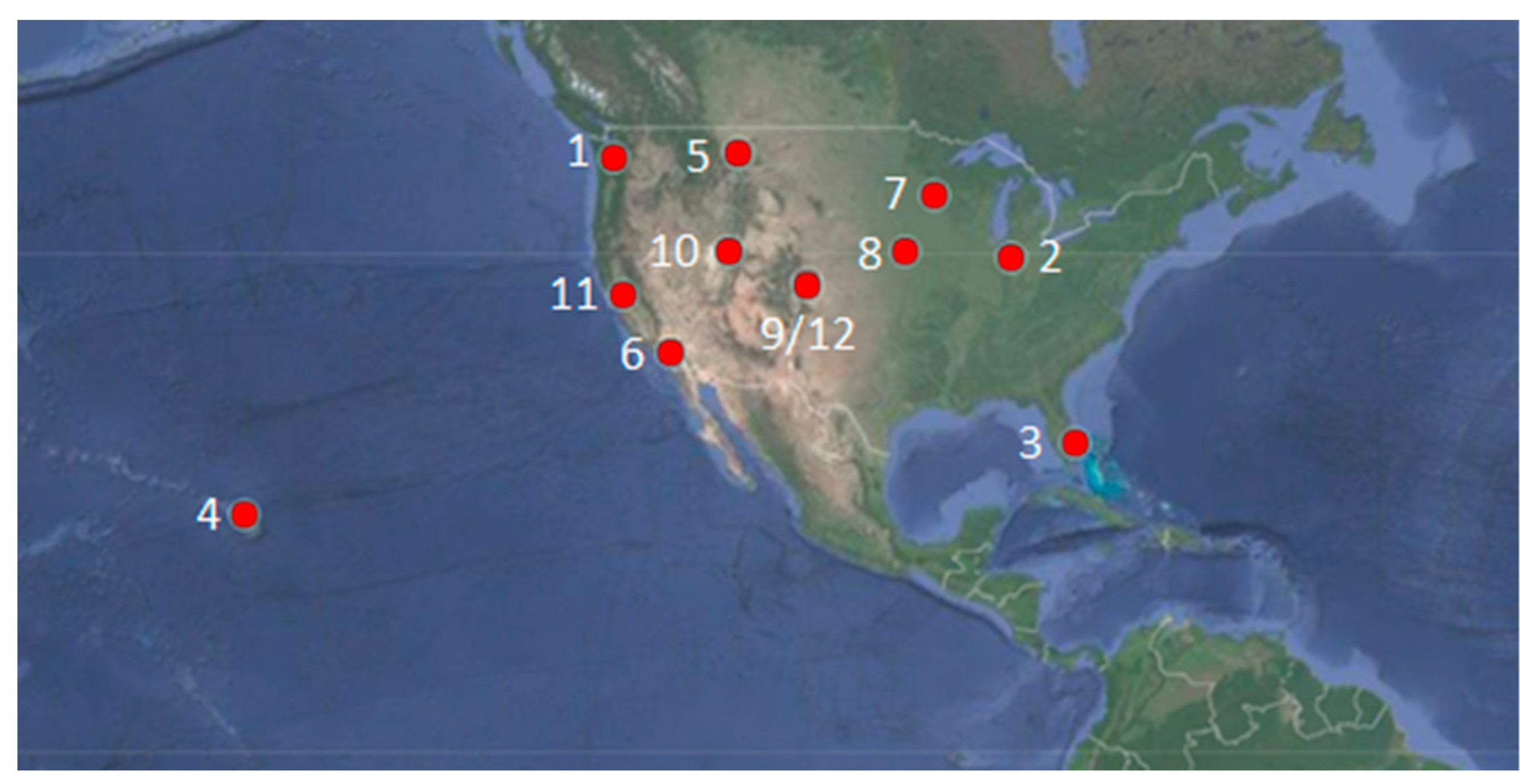
| Site | State | Latitude (deg) | Longitude (deg) | Köppen–Geiger Climate Region [40] |
|---|---|---|---|---|
| 1. Camp Murray | Washington | 47.11 | 122.57 | Csb |
| 2. Grissom | Indiana | 40.67 | 86.15 | Dfa |
| 3. JDMT | Florida | 26.98 | 80.11 | Cfb |
| 4. Kahului | Hawaii | 20.89 | 156.44 | Af |
| 5. Malmstrom | Montana | 47.52 | 111.18 | BSk |
| 6. March | California | 33.9 | 117.26 | Csa |
| 7. MNANG | Minnesota | 44.89 | 93.2 | Dfa |
| 8. Offutt | Nebraska | 41.13 | 95.75 | Dfa |
| 9. Peterson | Colorado | 38.82 | 104.71 | BSk |
| 10. Hill Weber | Utah | 41.15 | 111.99 | Dfb |
| 11. Travis | California | 38.16 | 121.56 | Csa |
| 12. USAFA | Colorado | 38.95 | 104.83 | BSk |
| Variable | Units | Minimum | 1st Quartile | Median | Mean | 3rd Quartile | Maximum |
|---|---|---|---|---|---|---|---|
| Power output | Watts | 0.3 | 6.4 | 13.8 | 13.0 | 18.9 | 34.3 |
| Latitude | Degrees | 20.89 | 38.16 | 38.95 | 38.12 | 41.15 | 47.52 |
| Humidity | Percent | 0 | 17.5 | 33.1 | 37.1 | 52.6 | 100 |
| Ambient temp | Celsius | −20.0 | 21.9 | 30.3 | 29.3 | 37.5 | 65.7 |
| Wind speed | km/h | 0 | 9.7 | 14.5 | 16.6 | 22.5 | 78.9 |
| Visibility | km | 0 | 16.1 | 16.1 | 15.6 | 16.1 | 16.1 |
| Pressure | Millibars | 781 | 845 | 961 | 925 | 1008 | 1029 |
| Cloud ceiling | km | 0 | 4.3 | 22 | 15.7 | 22 | 22 |
| Altitude | m | 0.3 | 0.6 | 140 | 244 | 417 | 593 |
| Machine Learning Technique | H2O.ai | Cross-Validation | ||
|---|---|---|---|---|
| R2 | MAE (W) | RMSE (W) | R2 | |
| DRF—Distributed random forest | 0.939 | 1.176 | 1.754 | 0.673 |
| XRT—Extremely randomized trees | 0.924 | 1.341 | 1.965 | 0.664 |
| Stacked ensemble build | 0.868 | 1.748 | 2.585 | 0.687 |
| GBM—Gradient boosting machine | 0.802 | 2.134 | 3.173 | 0.681 |
| Deep learning | 0.593 | 3.386 | 4.545 | 0.605 |
| GLM—Generalized linear model | 0.502 | 3.896 | 5.027 | 0.501 |
| Variable | Scaled Performance for 50 Trees | Scaled Performance for 500 Trees |
|---|---|---|
| Ambient temp | 100% | 100% |
| Humidity | 55% | 46% |
| Cloud ceiling | 52% | 42% |
| Month | 50% | 36% |
| Pressure | 26% | 24% |
| Time | 25% | 22% |
| Latitude | 25% | 21% |
| Wind speed | 19% | 17% |
| Visibility | 4% | 3% |
| Location | R2 | MAE (W) | RMSE (W) | First Variable | Value | Second Variable | Value |
|---|---|---|---|---|---|---|---|
| Camp Murray | 0.962 | 0.876 | 1.339 | Ambient Temp | 37% | Humidity | 26% |
| Grissom | 0.948 | 0.957 | 1.534 | Ambient Temp | 34% | Humidity | 23% |
| JDMT | 0.929 | 1.461 | 1.999 | Humidity | 27% | Ambient Temp | 24% |
| Travis | 0.968 | 0.779 | 1.193 | Ambient Temp | 29% | Humidity | 21% |
| Hill Weber | 0.955 | 0.988 | 1.445 | Ambient Temp | 27% | Humidity | 24% |
| Kahului | 0.908 | 1.699 | 2.187 | Humidity | 25% | Ambient Temp | 23% |
| Malmstrom | 0.951 | 1.023 | 1.564 | Ambient Temp | 32% | Humidity | 23% |
| Offutt | 0.937 | 1.456 | 2.038 | Humidity | 33% | Ambient Temp | 22% |
| USAFA | 0.924 | 1.160 | 1.609 | Ambient Temp | 21% | Cloud Ceiling | 16% |
| MNANG | 0.955 | 1.069 | 1.643 | Ambient Temp | 34% | Cloud Ceiling | 17% |
| Peterson | 0.947 | 1.050 | 1.561 | Ambient Temp | 30% | Humidity | 17% |
| March | 0.936 | 0.919 | 1.296 | Month | 23% | Ambient Temp | 23% |
| All Locations | 0.939 | 1.187 | 1.754 | Ambient Temp | 32% | Humidity | 15% |
| Measure | Present Work | Busquet et al. [35] | Kayri et al. [12] | Lahouar et al. [13] |
|---|---|---|---|---|
| Model | DRF | Linear regression | Random forest | Random forest |
| Dependent variable | Power | Daily energy | Power | Power |
| R2 | 0.939 | 0.87 * | 0.986 | N/A |
| MAE (W) | 1.176 | N/A | 2.376 | 30144 ** |
| RMSE (W) | 1.754 | N/A | N/A | 44343 ** |
| Importance—1st variable | Ambient temp | High/low irradiation | Global radiation | Solar irradiance ** |
| Importance—2nd variable | Humidity | Ambient temp | Solar elevation angle | Humidity ** |
| Importance—3rd variable | Cloud ceiling | Wind speed | Temperature | Temperature ** |
© 2020 by the authors. Licensee MDPI, Basel, Switzerland. This article is an open access article distributed under the terms and conditions of the Creative Commons Attribution (CC BY) license (http://creativecommons.org/licenses/by/4.0/).
Share and Cite
Pasion, C.; Wagner, T.; Koschnick, C.; Schuldt, S.; Williams, J.; Hallinan, K. Machine Learning Modeling of Horizontal Photovoltaics Using Weather and Location Data. Energies 2020, 13, 2570. https://0-doi-org.brum.beds.ac.uk/10.3390/en13102570
Pasion C, Wagner T, Koschnick C, Schuldt S, Williams J, Hallinan K. Machine Learning Modeling of Horizontal Photovoltaics Using Weather and Location Data. Energies. 2020; 13(10):2570. https://0-doi-org.brum.beds.ac.uk/10.3390/en13102570
Chicago/Turabian StylePasion, Christil, Torrey Wagner, Clay Koschnick, Steven Schuldt, Jada Williams, and Kevin Hallinan. 2020. "Machine Learning Modeling of Horizontal Photovoltaics Using Weather and Location Data" Energies 13, no. 10: 2570. https://0-doi-org.brum.beds.ac.uk/10.3390/en13102570