Enhanced Prediction of Solar Radiation Using NARX Models with Corrected Input Vectors

Abstract

The main objective of this work is to analyze and configure appropriately the input vectors to enhance the performance of NARX models to forecast solar radiation one hour ahead. For this study, Engle–Granger causality tests were implemented. Additionally, collinearity among the meteorological variables of the databases was examined. Different databases were used to test the contribution of these analyses in the improvement of the input vectors. For that, databases from three cities of Mexico with different climates were obtained, namely: Chihuahua, Temixco, and Zacatecas. These databases consisted of hourly measurements of the following variables: solar radiation (SR), wind speed (WS), relative humidity (RH), pressure (P), and temperature (T). Results showed that, in all three cases, proper NARX models were produced even when using input vectors formed only with solar radiation and temperature data. Consequently, it was inferred that pressure, wind speed, and relative humidity could be excluded from the input vectors of the forecasting models since, according to the causality tests, they did not provide relevant information to improve the solar radiation forecast in the studied cases. Conversely, these variables could generate spurious results. Forecasting results obtained with the NARX model were compared to the smart persistence model, commonly used to validate SR prediction. Error measures, such as mean absolute error (MAE) and root mean squared error (RMSE), were used to compare prediction results obtained from different models. In all cases, results obtained from the enhanced NARX model surpassed the results of the smart persistence, namely: in Chihuahua up to $11.5\%$, in Temixco up to $15.7\%$, and in Zacatecas up to $27.2\%$.

1. Introduction

Solar radiation (SR) is the driving force behind several solar energy devices, such as photovoltaic systems for generating electricity and solar collectors for water heating [1]. Therefore, SR prediction models are essential for different applications, from the operation of energy systems (PV and thermal systems) to meteorological applications [2,3].

Several research works’ scope was to develop models that allowed predicting SR with acceptable precision. The techniques used in the forecast models varied according to the place and the available data, so it was difficult to classify them adequately. However, they could be divided into three main groups: clarity index models, hybrid models, and artificial neural network (ANN) models. In the first, the variable to model is the atmospheric transmittance or clarity index [4,5,6,7,8]. Hybrid models include those that combine a prediction model with data grouping techniques, such as the model used by Azimi et al. [9], which is a combination of a grouping technique and multilayer perceptron k-means ANN. Other authors have proposed hybrid models that use different types of ANN [10,11]. Recently, new hybrid models were developed, for example of the ARMA/ANN type, where different order ARMA models and several kinds of ANN have been used. In those cases, it is important to note that the ARMA model was used to deal with the linear part, while the ANN model was employed to forecast the non-linear part of the time series [10,12]. In some hybrid cases, the clarity index was also considered, like in the approach used by Voyant et al. [13]. Currently, ANN techniques are widely used in SR forecasting models. Sfetsos and Coonick [1] compared traditional linear methods against several artificial intelligence (AI) based techniques and found that AI models predicted the time series of solar radiation more effectively compared to conventional procedures; the feed-forward neural network (FFNN), Elman recurrent neural network, and diverse training functions were applied. Other examples of the use of FFNN to predict SR can be consulted in the bibliography [3,14,15]. In some research works, dividing the annual time series into seasonal time series was proposed [4,13,16]. Less conventional models were proposed by Pandey and Soupir [17] and Yang et al. [18], which included the use of polynomial expressions for the decomposition of the time series, the zenith angle, and the transmission function. An ARMA-time delay neural network (TDNN) hybrid model, based on data segmentation and a grouping algorithm, was developed for the hourly forecast of global solar radiation by Wu and Chan [19]. Huang et al. [20] used a coupled model of autoregressive and dynamic systems, obtaining a hybrid model, which they compared with the Lucheroni model.

Hocaoglu and Karanfil [21] proposed the use of causality tests to find the bidirectional relationship between the meteorological variables. In their study, wind speed, pressure, and temperature were used; however, the authors did not implement any forecast model. Ahmad et al. [22] used the Pearson correlation coefficient as a measure of the linear correlation between two variables to select the inputs of a prediction model, then the authors decided to try several combinations of inputs to obtain the global horizontal irradiation (GHI). Meanwhile, Aguiar et al. [23] proposed an ANN to forecast the GHI using the Pearson correlation to find the relationship between the satellite and terrestrial data to obtain the best input data to the ANN models.

The literature review showed that, in most cases, the entries of forecast models were intuitively selected. Furthermore, from the study on the state-of-the-art concerning hourly prediction of SR, the importance of the architecture and the performance of forecast models were evident. However, there was little information on the selection of the input variables of these models, and there was not a clear proposal on how these input variables should be chosen, with only a few works dealing with this topic.

The present research work focuses on the use of causality tests to find the proper inputs of multi-variable models for SR prediction, with a horizon of one hour; this implies that for the model to trace a synthetic time series, it always needs previous actual data of the input variables. Several NARX models were developed for three sites. In the first instance, the models included all variables in the input vector. Later, new models with input vectors built using the collinearity and causality tests were produced. All results were compared with the smart persistence model. The analysis of the results suggested that it was necessary to apply co-integration tests to the meteorological variables of each site database. The reason was that, in some cases, it was not necessary to include all variables as inputs for the forecast models. Therefore, these tests ensured avoiding spurious forecasts generated by a mistaken conformation of the multi-variable models of any kind: NARX, autoregressive vectors, ANN, etc. The structure of this document is the following: Section 2 presents a description of the studied sites’ datasets and the type of available meteorological variables. Afterwards, the theoretical bases for smart persistence, NARX models, Engle–Granger tests, and performance tests used to evaluate the forecast models are described in Section 3. In Section 4, the selection of input variables and the structure of the nonlinear autoregressive exogenous model (NARX) are presented and explained. Section 5 shows the results and the corresponding discussion.

2. Meteorological Variables’ Databases

Data from three sites were analyzed, and at each site, there was an available weather station with specific characteristics. The studied sites were chosen based on their solar radiation potential, weather characteristics, and data availability. These meteorological stations were located in different cities of Mexico, namely: Chihuahua, Temixco, and Zacatecas. Figure 1 shows an approximate climate map of Mexico. This figure also shows the locations of the studied sites. Furthermore,

Table 1. Location of meteorological stations and the weather type of the sites.

Site	Latitude	Longitude	Elevation	Weather
	(North)	(West)	(m.a.s.l.)	Type
Chihuahua	${28.6}^{\circ }$	${106.0}^{\circ }$	1415	Very dry
Temixco	${18.8}^{\circ }$	${99.2}^{\circ }$	1313	Warm-sub humid
Zacatecas	${22.8}^{\circ }$	${102.6}^{\circ }$	2460	Dry

shows the precise location of the sites and their corresponding weather type. The main characteristics of measurement equipment of the meteorological stations are shown in

Table 2. Sensor characteristics.

Probe	Sensor	Range	Accuracy
Eppley B&W Pyranometer	–	–	–
CS500 Temperature Probe	1000 $\mathsf{\Omega }$ platinum resistance	$-{40.0}^{\circ }$C to $+60.0{}^{\circ }$C	$\pm 0.5{}^{\circ }$C
	thermometer, DIN43760B
CS500 Relative Humidity Probe	Vaisala INTERCAP	0 to $100\%$	$\pm 3\%$
R.M. Young Wind Sentry Anemometer	Cups Wheel Assembly	$0.0$ to $50.0$ m/s	$\pm 0.5$ m/s
PTB110 Barometer	Vaisala BAROCAP	$500.0$–$1100.0$ hPa	$\pm 0.3$ hPa
WXT510 Weather Transmitter	Ultrasonic Signal	0 to 60 m/s	$3\%$
	BAROCAP	600 to 1100 hPa	$\pm 0.5$ hPa
	THERMOCAP Sensor	$-52.0{}^{\circ }$C to $60.0{}^{\circ }$C	$\pm 0.3{}^{\circ }$C
	HUMICAP Sensor	0 to $100\%$ RH	$\pm 3\%$ RH

.

Three databases containing 17,520 hourly measurements of each variable, that is two full years of data, were consulted; however, due to the databases’ restrictions, different years were employed. In the case of Chihuahua, four meteorological variables were monitored: solar radiation, temperature, relative humidity, and pressure (SR, T, RH, and P); from January 2014 to December 2015. In the case of Temixco, five meteorological variables were measured: SR, T, RH, P, and wind speed (WS); from January 2013 to December 2014. Finally, for the case of Zacatecas, four meteorological variables were monitored: SR, T, RH, and WS; from January 2006 to December 2007.

3. Techniques and Methods Used in the Analysis

This section describes the applied techniques to select the data that formed the input vectors of the NARX models to forecast SR.

3.1. Collinearity Tests

Two variables are defined as collinear if the data vectors that represent them are on the same line (i.e., subspace of dimension one). Generally, the k variables are collinear if the vectors that represent them are in a subspace of dimension smaller than k, that is if one of the vectors is a linear combination of the other vectors. In practice, such “exact collinearity” rarely occurs, but this is certainly not necessary to consider that a collinearity problem exists [24].

Usually, an analysis of the principal components of the independent variables is performed to detect the collinearity. The principal components of a set of variables to other variables are referred to as the linear combination of the original variables. The principal components have three properties: (a) they are mutually independent (they are not correlated with each other); (b) they maintain the same information as the original variables; (c) they have the maximum variance with the above limitations. The variance of each principal component is an eigenvalue of the variance-covariance matrix of the original variables.

The number of null eigenvalues indicates the number of variables that are a linear combination of others (the number of exact collinearities). The eigenvalues near zero indicate serious collinearity problems.

3.2. Engle–Granger Causality Test

The fundamental aim of the co-integration tests is to know how much useful information the input variables provide to the model. This information is used to decide which variables should be part of the forecasting model. One of the most popular co-integration tests is the Engle–Granger causality method.

The causality test avoids the generation of spurious results, with a certain level of precision (in this study, a confidence level of $1\%$ was used). By eliminating unnecessary variables from the forecast model, the inclusion of meteorological variables that do not provide any significant information could be avoided; such variables may affect the model performance in unexpected or unwanted ways. These results are the spurious phenomenon of the nonsense regression explained by Yule [25]. Yule proved that spurious correlation could persist in non-stationary time-series, even if the sample is very large.

The Engle–Granger causality tests propose a hypothesis diagnostic, where the null hypothesis rejects the causality approach of one variable against another variable, that is the independent variable does not have useful information to predict the dependent variable. The Engle–Granger causality tests first assumes that the variable X does not cause the variable Y. If this null hypothesis is rejected, then the variable X causes the variable Y, that is the variable X contains relevant information to predict the variable Y. The causality tests were carried out by solving Equations (1) and (2).

$$Y_t=\sum _{i=1}^n{\alpha }_i{X}_{t-i}+\sum _{j=1}^n{\beta }_j{Y}_{t-j}+u_{1t},$$

(1)

$$X_t=\sum _{i=1}^n{\lambda }_i{Y}_{t-i}+\sum _{j=1}^n{\delta }_j{X}_{t-j}+u_{2t},$$

(2)

where X is, for example, the solar radiation, Y is the air temperature, $u_{1t}$ is the uncorrelated white noise, and n is the number of lags. ${\alpha }_i$, ${\beta }_j$, ${\lambda }_i$, and ${\delta }_j$ are parameters to be determined.

Similarly, using the auto-regressive vector technique, it is possible to elaborate tests for several variables [25]; such as wind speed, relative humidity, etc.

Since the results of the causality test depend on the number of lags, these tests were conducted using $2,3,\dots ,$ and 24 lags. The results were considered acceptable when some of the unnecessary variables were rejected after modifying the number of lags, due to the main objective of this work being fulfilled: to develop SR forecasting models with a reduced number of input variables.

3.3. Augmented Dickey–Fuller Test

Many statistical tests that help to determine if a time-series is or is not stationary exist. The augmented Dickey–Fuller (ADF) test was implemented in this work to identify the stationarity of the time-series. This test is based on the null hypothesis, which supposes that an analyzed time-series is non-stationary. Still, if this first hypothesis is rejected, then the time-series is considered stationary.

On the other hand, unit root tests are based on the study of stochastic time-series; in this case: pure random walk, random walk with drift, and random walk with drift and deterministic trend. Furthermore, the random walk with drift and deterministic trend model was proposed with an additional term, which considered whether the term $u_t$ was correlated or not [25], as can be seen in Equation (3).

$$\Delta Y_t={\beta }_1+{\beta }_{2}t+\delta Y_{t-1}+\sum _{i=1}^m{\alpha }_j\Delta Y_{t-j}+{ϵ}_t,$$

(3)

where ${\beta }_1$ is the drift, ${\beta }_2$ is the deterministic trend term, $\delta$ is the term that indicates if the time-series is stationary, ${ϵ}_t$ is a pure error term, and $\Delta Y_{t-i}=\left(Y_{t-1}-Y_{t-2}\right)$, $\Delta Y_{t-2}=\left(Y_{t-2}-Y_{t-3}\right)$, etc.

3.4. Non-Linear Auto-Regressive Model with Exogenous Inputs

Consider a recurrent neural network with only one input and one output, whose behavior is described by Equations (4) and (5). Given this state-space model, modifying it into an input-output model as an equivalent representation of the neural network is necessary.

$$x(n+1)=\varphi \left[W_{a}x\left(n\right)+w_{b}u\left(n\right)\right],$$

(4)

$$y\left(n\right)=c^{T}x\left(n\right).$$

(5)

Using Equations (4) and (5), it can be easily demonstrated that the output $y(n+q)$ could be expressed in terms of the state $x\left(n\right)$ and the input vector $u_q\left(n\right)$ as follows:

$$y(n+q)=\mathsf{\Phi }\left[x\left(n\right),u_q\left(n\right)\right],$$

(6)

where q is the dimensional form of the state-space model and $\mathsf{\Phi }:{\Re }^{2q}\to \Re$. Provided that the recurrent network is observable, the local observability theorem can be used to write:

$$x\left(n\right)=\mathsf{\Psi }[y_p\left(n\right),u_{q-1}\left(n\right)],$$

(7)

where $\mathsf{\Psi }:{\Re }^{2q-1}\to {\Re }^q$. Hence, substituting Equation (7) in Equation (6), it is obtained:

$$\begin{array}{ccc}\hfill y(n+q)& =& \mathsf{\Phi }\left[\mathsf{\Psi }\left(y_p\left(n\right),u_{q-1}\left(n\right)\right),u_q\left(n\right)\right]\hfill \\ & =& F\left[y_q\left(n\right),u_q\left(n\right)\right],\hfill \end{array}$$

(8)

where $u_{q-1}\left(n\right)$ is contained in $u_q\left(n\right)$ as its first elements ($q-1$), and the nonlinear mapping $F:{\Re }^{2q}\to \Re$ takes care of both $\varphi$ and $\psi$.

$$u_{q-1}\left(n\right)={\left[u\left(n\right),u(n+1),\cdots ,u(n+q-2)\right]}^T,$$

(9)

$$y_p\left(n\right)={\left[y\left(n\right),y(n+1),\cdots ,y(n+q-1)\right]}^T.$$

(10)

Using the definitions of $y_p(n$) and $u_q\left(n\right)$ given in Equations (9) and (10), we may rewrite Equation (8) as the expanded form:

$$y(n+q)=F\left[y(n+q-1),\cdots ,y\left(n\right),u(n+q-1),\cdots ,u\left(n\right)\right].$$

(11)

Replacing n with $n-q+1$, then:

$$y(n+1)=F\left[y\left(n\right),\cdots ,y(n-q+1),u\left(n\right),\cdots ,u(n-q+1)\right].$$

(12)

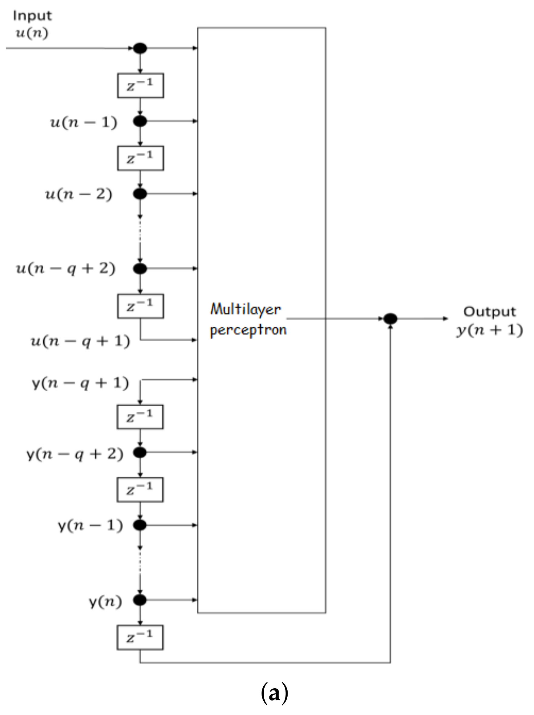
Expressed in words, some non-linear mapping $F:{\Re }^{2q}\to \Re$ exists whereby the present value of the output $y(n+1)$ is uniquely defined in terms of its past values $y\left(n\right),\cdots ,y(n-q+1)$ and the present and past values of the input $u\left(n\right),\cdots ,u(n-q+1)$. For this input-output representation to be equivalent to the state-space model of Equations (4) and (5), the recurrent network must be observable. The practical representation of this equivalence is that the NARX model (see Figure 2a, with its limited feedback towards the output neuron, is in fact able to simulate the corresponding fully recurrent state-space model of Figure 2b (assuming that $m=1$ and $p=1$), with no difference between their input-output behavior [26].

3.5. Smart Persistence Model

The smart persistence model was used as a benchmark. Despite the simplicity of this model, it can be very accurate for low variability periods. Therefore, the smart persistence model is useful to compare to other models. This model is defined as [27]:

$$SR(t+\Delta t)=\frac{S{R}_{clr}(t+\Delta t)}{S{R}_{clr}\left(t\right)}SR\left(t\right).$$

(13)

It is well known that solar radiation suffers losses due to dispersion and atmospheric absorption when it passes through the atmosphere [28]. After the atmospheric absorption phenomenon, the normal solar flow rate (solar radiation/normal irradiance) that reaches the Earth’s surface is calculated with Equation (14), found in the Handbook of Solar Energy [28], where it is also mentioned that SR can be another form of normal irradiance.

$$S{R}_{clr}=I_{ext}·exp\left[-\frac{T_R}{\left(0.9+9.4·cos{\theta }_z\right)}\right],$$

(14)

and:

$$cos{\theta }_z=cos\varphi cos\delta cos\omega +sin\delta sin\varphi ,$$

(15)

where ${\theta }_z$ is the solar zenith angle defined as the angle between the vertical and the line connecting to the Sun, $I_{ext}$ is the extraterrestrial irradiance per hour, $T_R$ is the turbidity factor, $\varphi$ is the latitude of the site, $\delta$ is the declination angle of the Earth, and $\omega$ is the hour angle.

The extraterrestrial hourly mean irradiance (W/m${}^2$) is calculated by the following equation [29]:

$$I_{ext}=I_{sc}{E}_0(sin\delta sin\varphi +0.9972·cos\delta cos\varphi cos{\omega }_{0.5}),$$

(16)

where $E_0$ is the eccentricity correction factor, $I_{sc}=1367$ W/m${}^2$ is the solar constant, and ${\omega }_{0.5}$ is the hour angle at the half hour.

3.6. Solar Radiation Estimation under Clear Sky Conditions, $S{R}_{clr}$

To have a reference and a constraint for the calculation of smart persistence, a monthly ideal turbidity factor was calculated for each site by solving Equation (14) for $T_R$:

$$T_R=-log\left[\frac{{\left(SR\right)}_{month}}{{\left(I_{ext}\right)}_{month}}\right]·\left[0.9+9.4·{(cos{\theta }_z)}_{month}\right],$$

(17)

where ${\left(SR\right)}_{month}$ is the maximum value of the month of solar irradiance measured at each site, ${\left(I_{ext}\right)}_{month}$ is the maximum value of solar extraterrestrial radiation for each month at each site, and ${(cos{\theta }_z)}_{month}$ is the monthly value used to calculate ${\left(I_{ext}\right)}_{month}$ according to [28].

Table 3. Turbidity factor, $T_R$, in Chihuahua, Chih.

	Jan.	Feb.	Mar.	Apr.	May.	Jun.	Jul.	Aug.	Sept.	Oct.	Nov.	Dec.
${\left(I_{ext}\right)}_{month}$, (W/m${}^2$)	986	1128	1267	1337	1352	1352	1349	1337	1285	1172	1018	904
${\left(SR\right)}_{month}$, (W/m${}^2$)	784	946	1037	1068	1100	1087	1051	1046	1013	909	778	767
${(cos{\theta }_z)}_{month}$, (−)	0.680	0.786	0.897	0.962	0.986	0.986	0.988	0.975	0.926	0.831	0.710	0.623
$T_R$, (−)	1.672	1.464	1.869	2.236	2.099	2.225	2.545	2.468	2.283	2.213	2.035	1.111

,

Table 4. Turbidity factor, $T_R$, in Temixco, Mor.

	Jan.	Feb.	Mar.	Apr.	May.	Jun.	Jul.	Aug.	Sept.	Oct.	Nov.	Dec.
${\left(I_{ext}\right)}_{month}$, (W/m${}^2$)	1153	1261	1351	1375	1374	1359	1360	1362	1351	1287	1175	1085
${\left(SR\right)}_{month}$, (W/m${}^2$)	864	950	1011	1039	1017	1043	1056	1026	1103	950	840	816
${(cos{\theta }_z)}_{month}$, (−)	0.795	0.879	0.957	0.989	0.990	0.991	0.992	0.990	0.973	0.912	0.811	0.748
$T_R$, (−)	2.412	2.597	2.867	2.851	3.074	2.706	2.588	2.890	2.040	2.875	2.882	2.261

and

Table 5. Turbidity factor, $T_R$, in Zacatecas, Zac.

	Jan.	Feb.	Mar.	Apr.	May.	Jun.	Jul.	Aug.	Sept.	Oct.	Nov.	Dec.
${\left(I_{ext}\right)}_{month}$, (W/m${}^2$)	1091	1213	1323	1365	1366	1361	1356	1356	1330	1246	1117	1017
${\left(SR\right)}_{month}$, (W/m${}^2$)	642	720	798	888	834	985	897	860	867	795	575	584
${(cos{\theta }_z)}_{month}$, (−)	0.752	0.845	0.937	0.982	0.988	0.993	0.991	0.989	0.958	0.883	0.779	0.701
$T_R$, (−)	4.228	4.617	4.905	4.356	5.034	3.311	4.230	4.648	4.237	4.140	5.461	4.155

show the obtained results from Equation (17) of the turbidity factor, $T_R$, corresponding to Chihuahua, Temixco, and Zacatecas, respectively.

It is worth mentioning that it was only necessary to calculate $T_R$ once for each month since the maximum value measured in each month of both SR and $I_{ext}$ was used. The maximum ideal SR could be calculated using a single $T_R$ under optimal conditions at each site per month. The goal was to use that SR calculated value as a constraint for the smart persistence model so that it never exceeded such a value.

Note that the results for the turbidity factor were obtained under the following hypotheses:

• at least one day of each month had clear sky conditions.
• SR obtained under clear sky conditions was calculated by considering the maximum irradiance of every month.

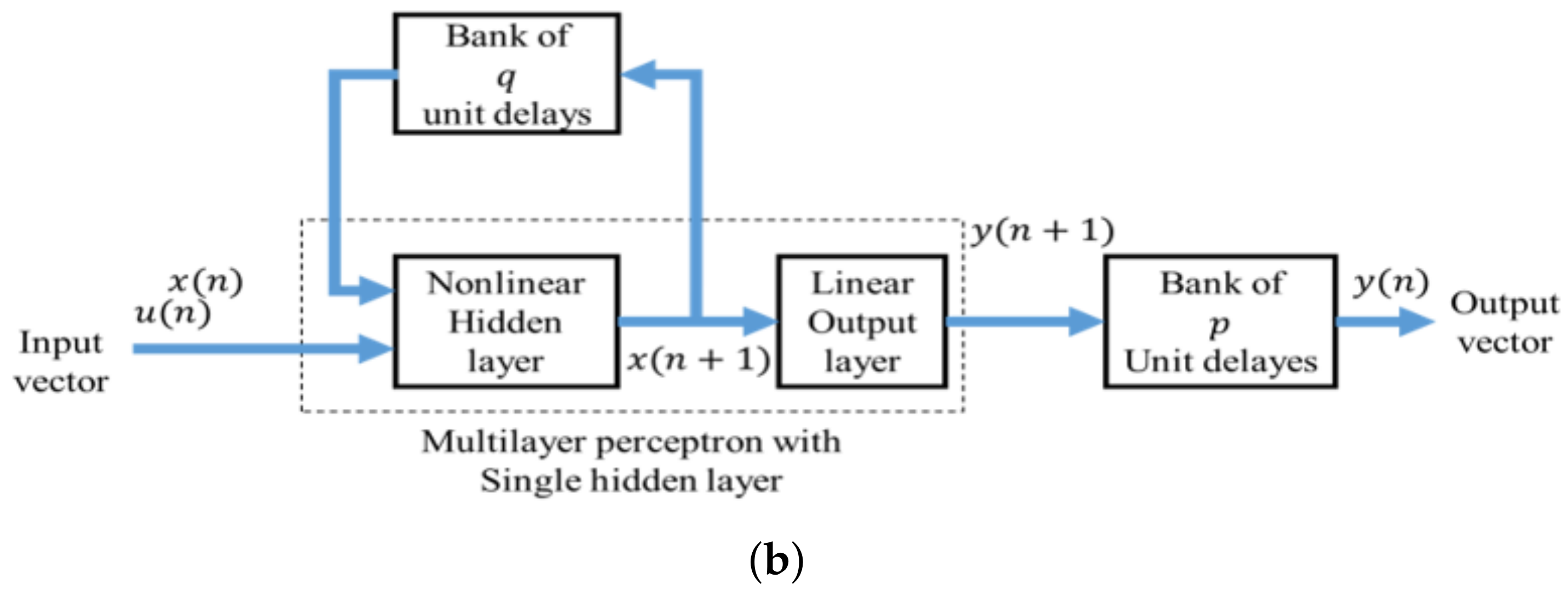
Figure 3 presents the synthetic series of maximum ideal $S{R}_{clr}$ generated using Equation (14) for a typical year, where the monthly $T_R$ presented in Table 3, Table 4 and Table 5 was used. It should be noticed that 8760 computed data of $S{R}_{clr}$ were plotted from hourly known values of $I_{ext}$ and ${\theta }_z$ for each site, which were adjusted by $T_R$ for each month at each site, specifically. This figure also shows the first 744 h corresponding to January, where 31 peaks can be easily observed, one for a day. Several interesting phenomena were observed when reviewing the entire synthetic series: first, it seemed that a relatively continuous area was drawn; however, it was not: it was a line graph that, being a series of hourly $S{R}_{clr}$, had a cyclical shape with very close waves; second, 12 steps appeared, due to the effect of $T_R$, which scaled the results and changed every month; and finally, a trend was observed in the data that corresponded to the annual seasonal cycle where the summer months received more $S{R}_{clr}$. It is important to highlight that $T_R$ produced a peculiar behavior in Zacatecas since there was a significant gap from June to August compared to the rest of the year.

3.7. Performance Tests

Two standard error metrics widely used in the solar prediction area were implemented: the root mean squared error (RMSE) and the mean absolute error (MAE).

$$RMSE=\sqrt{\frac{1}{n}\sum _{i=1}^n{\left({\left(SR\right)}_f-{\left(SR\right)}_m\right)}^2},$$

(18)

$$MAE=\frac{1}{n}\sum _{i=1}^n\left|{\left(SR\right)}_f-{\left(SR\right)}_m\right|,$$

(19)

where ${\left(SR\right)}_f$ is the forecasted solar radiation and ${\left(SR\right)}_m$ is the measured solar radiation.

Additionally, to compare the relative improvement of the different models with respect to the smart persistence model, the forecast skill parameter was calculated as defined in [23].

$$Forecas{t}_{skill}(\%)=\left(1-\frac{RMS{E}_{NARX}}{RMS{E}_{SP}}\right)·100,$$

(20)

where the subscripts ${}_{NARX}$ and ${}_{SP}$ denote the NARX model and the smart persistence model, respectively.

4. Selection of Input Variables and the Structure of the NARX Model

This section explains how the collinearity and co-integration tests were applied to assemble the input vectors of the prediction model. Afterwards, the general architecture of a trained NARX model is presented.

4.1. Collinearity Tests

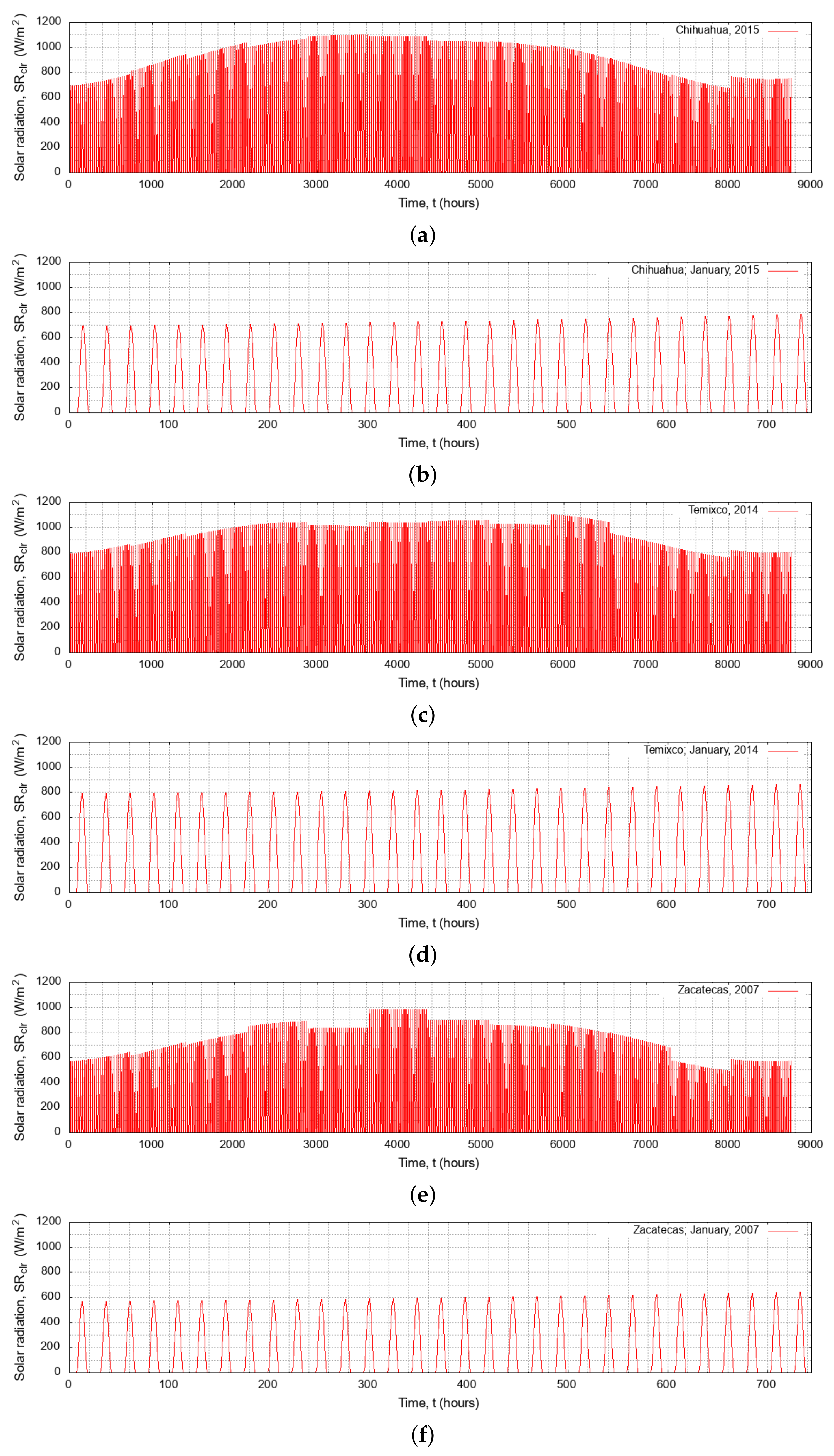
When a variable has a linear combination with another one, it means that both variables are related through a linear expression. When the linear correlation coefficient between the variables is equal to unity, the variables have a simple collinearity. In the case of multiple variables, collinearity occurs when some independent variables are correlated with each other. One way to detect collinearity between multiple variables is through principal component analysis of the independent variables. The variance of each principal component is an eigenvalue of the variance-covariance matrix of the original variables. The null eigenvalues indicate the number of variables that are linear combinations of others (exact collinearities). Once the presence and number of collinearities are determined in a multivariate time-series, it is convenient to find the involved variables through the calculation of their variance-decomposition proportion for each component; Belsley et al. [24] proposed using a proportion threshold of about $0.5$.

Collinearity tests were used to assemble the input vectors of the NARX models correctly. Figure 4 shows the collinearity tests performed on the multivariate time series of the three studied sites, with the available variables in each site, namely:

• In the case of Chihuahua, the temperature and the pressure were above the threshold of the variance-decomposition proportion; see Figure 4a. Thus, in the next stage, the collinearity tests were performed omitting one of these variables, obtaining two new combinations of input vectors. The first input vector was assembled using SR, RH, and T. The second vector was constructed using SR, RH, and P.
• In the case of Temixco, temperature, relative humidity, and pressure showed collinearity; see Figure 4b. Therefore, three new input vectors were obtained formed as follows: SR, WS, and T variables for the first vector; SR, WS, and RH variables for the second vector; and SR, WS, and P variables for the third vector.
• In the case of Zacatecas, the temperature significantly exceeded the threshold of 0.5; see Figure 4c. Therefore, two new input vectors were obtained in combination with the temperature, i.e., SR, RH, and T; and SR, WS, and T.

Table 6. Input vectors of Chihuahua, Chih.

Vector	Input Variables	Output Variable	Tests
1	SR, RH, T, P	SR	–
2	SR, RH, T	SR	Collinearity
3	SR, RH, P	SR	Collinearity
4	SR, T	SR	Collinearity and cointegration

,

Table 7. Input vectors of Temixco, Mor.

Vector	Input Variables	Output Variable	Tests
1	SR, WS, T, RH, P	SR	–
2	SR, WS, T	SR	Collinearity
3	SR, WS, RH	SR	Collinearity
4	SR, WS, P	SR	Collinearity
5	SR, T	SR	Collinearity and cointegration

and

Table 8. Input vectors of Zacatecas, Zac.

Vector	Input Variables	Output Variable	Tests
1	SR, RH, WS, T	SR	–
2	SR, RH, T	SR	Collinearity
3	SR, WS, T	SR	Collinearity
4	SR, T	SR	Collinearity and cointegration

show the proposed input vectors for Chihuahua, Temixco, and Zacatecas, respectively. In all cases, Vector 1 was formed using all available meteorological variables. Vectors 2 and 3 (and 4 for Temixco) were obtained from the results of the collinearity tests. Finally, Vector 4 (5 for Temixco) was the result of the application of collinearity and integration tests.

4.2. Engle–Granger Causality Tests

Cointegration tests to identify redundant variables of the input vector built from collinearity test were applied. In the case of Chihuahua, the collinearity test determined two different combinations of input vectors: $V_2=[SR,RH,T]$ and $V_3=[SR,RH,P]$; which were formed using separately the variables that presented collinearity. Then, the causality test was applied to $V_2$, identifying the RH as a redundant variable, so the RH was eliminated from the this input vector, obtaining $V_4=[SR,T]$ of Table 6. For $V_3$, the test did not register any redundant variable, so the input variables remained the same.

In the case of Temixco, the causality tests were applied to three groups of input variables: $V_2=[SR,WS,T]$, $V_3=[SR,WS,RH]$, and $V_4=[RS,WS,P]$. The tests indicated that there would only be a change in the case of $V_2$, where it was determined that the WS was a redundant variable. Therefore, the new vector $V_5=[SR,T]$ of Table 7 was defined.

Finally, in the city of Zacatecas, it was found that only T showed collinearity, and two input vectors were formed:

$V_2=[SR,T,RH]$, $V_3=[SR,T,WS]$. The causality tests determined the relative humidity as a redundant variable in $V_2$. Therefore, the new input vector $V_4=[SR,T]$ was formed; see Table 8.

4.3. NARX Models Including Collinearity Tests

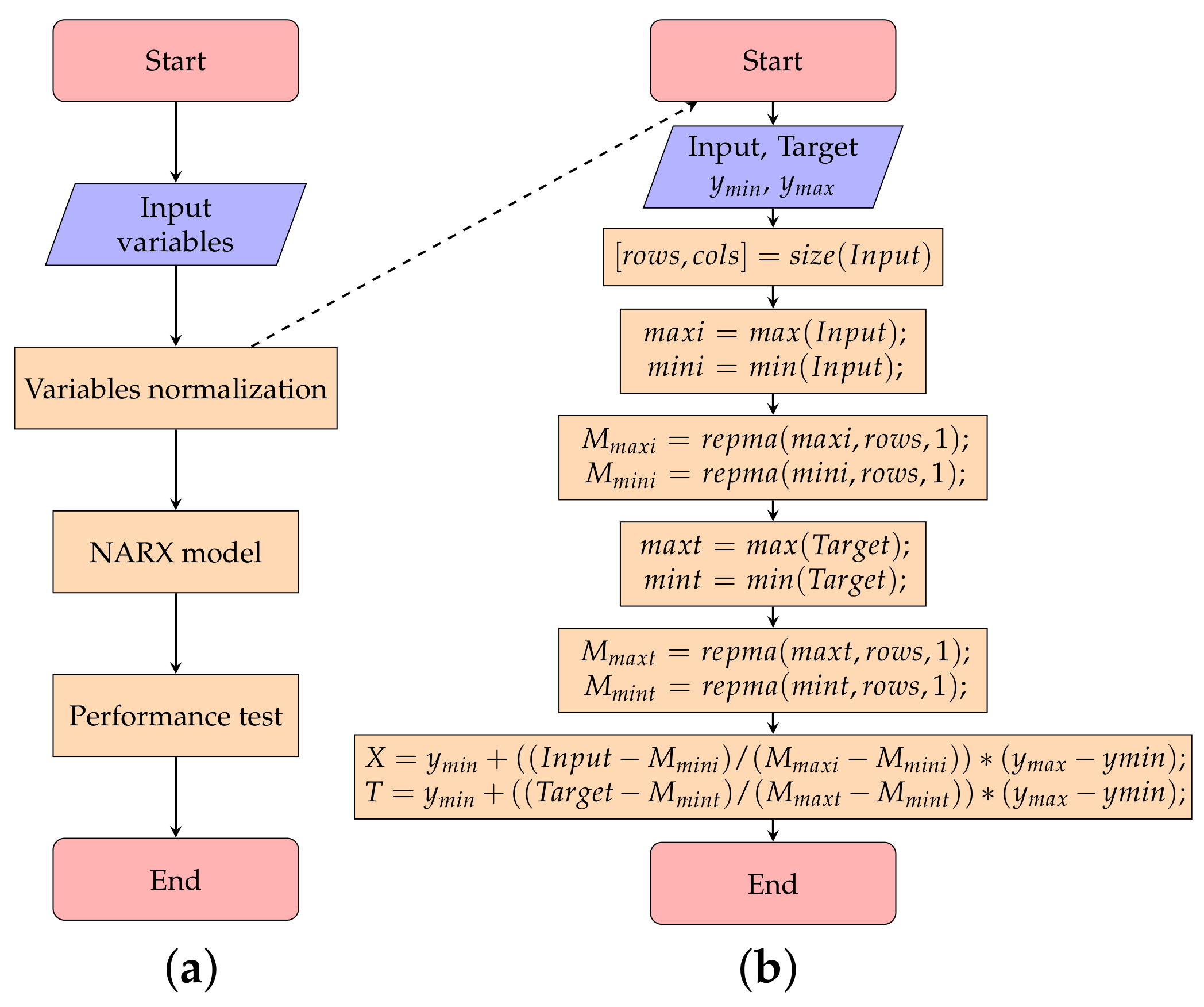
Once the input vectors were determined, the NARX models were developed for each of the cases shown in Table 6, Table 7 and Table 8. When all the meteorological variables were used (i.e., vectors $V_1$), as well as vectors obtained from the causality tests, the NARX models were performed using the diagram of Figure 5. The flowchart initiated when input variables were entered. Then, the NARX model was trained, and finally, the performance tests were calculated. The variables were normalized with values from zero to one, before the NARX model was trained. To normalize the variables, the subroutine shown in Figure 5b was used.

4.4. NARX Models Including Collinearity and Engle–Granger Causality Tests

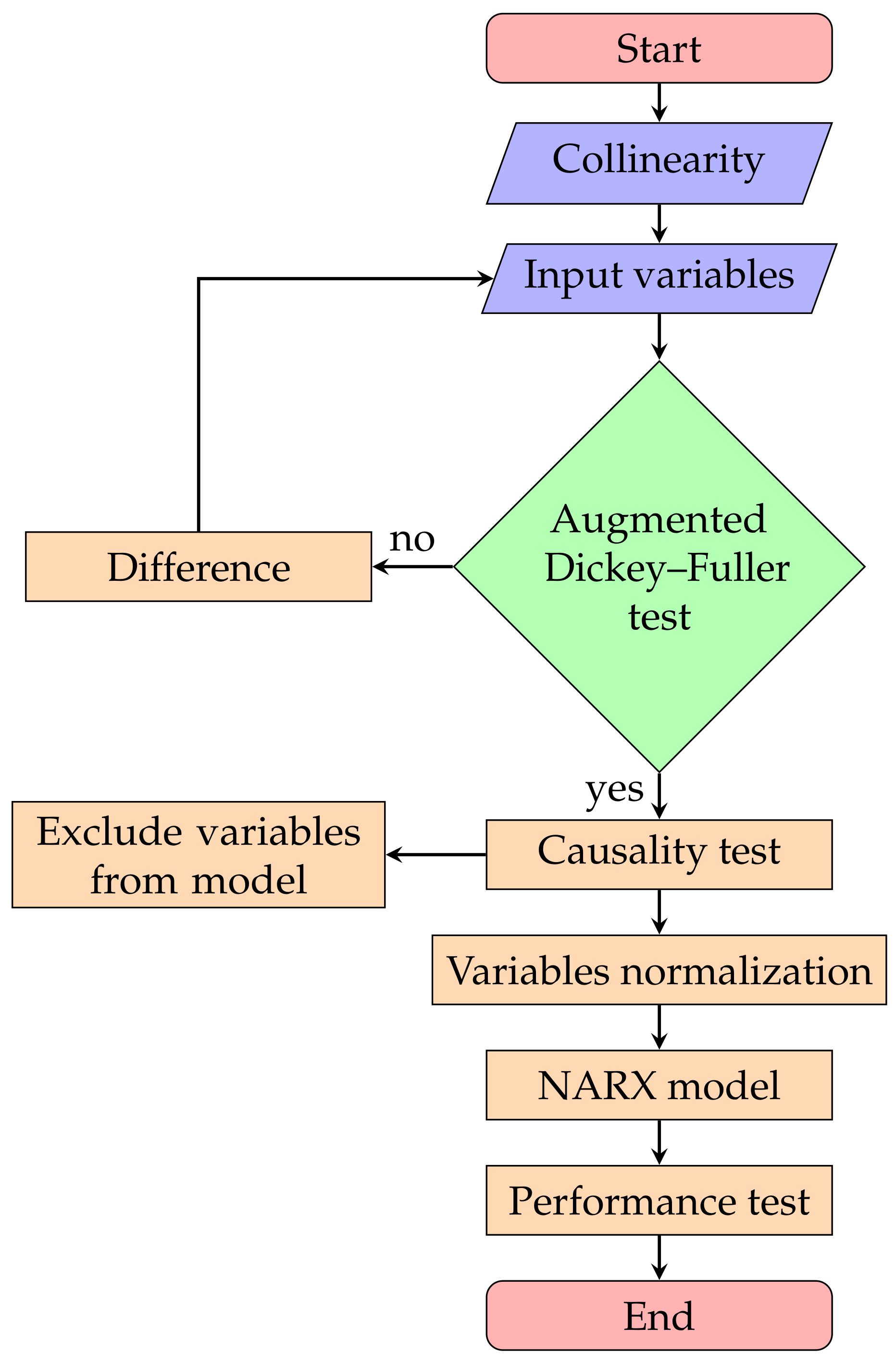
The main objective of this research work was to build the best NARX model, based on the proper input vectors. The flowchart of Figure 6 shows the steps that were followed to define the relevant variables in the solar radiation prediction using collinearity and causality tests. In the case of Chihuahua, $V_1$ included all the variables. Then, $V_2$ and $V_3$ were obtained, applying the collinearity test. Finally, the causality test was applied on both input vectors, showing a difference only in $V_2$. This test indicated that the RH did not cause SR. Therefore, the new input vector was formed as $V_4=[SR,T]$. In the case of Temixco, the causality test was used to build $V_2$, $V_3$, and $V_4$. The causality test determined that the WS did not cause SR in $V_2$, while in $V_3$ and $V_4$, there was no change, that is the input vectors remained the same. Therefore, the new input vector was formed as $V_5=[SR,T]$. For Zacatecas, the causality test was implemented in $V_2$ and $V_3$. From the application of this test, only $V_2$ determined that the HR did not cause SR, while in Case 3, no change was registered in the input variables, resulting in $V_4=[SR,T]$.

According to the obtained results from the collinearity and causality tests’ application, the proper input vector for each site only included SR and T, that is one non-collinear variable and one collinear variable.

Although preliminary results indicated that the best input vector only included SR and T, NARX models were trained for each of the cases from Table 6, Table 7 and Table 8 to compare all NARX models through the performance tests, in which it was expected that those NARX models with the best input vector would obtain the best forecast performance. The first year of the available data was used as the training data. For the performance tests, the SR forecast horizon was one hour ahead. These results were compared with the second year of the data measured in each of the sites, i.e., a blind forecast was calculated.

4.5. Number of Time Lags of the NARX Model

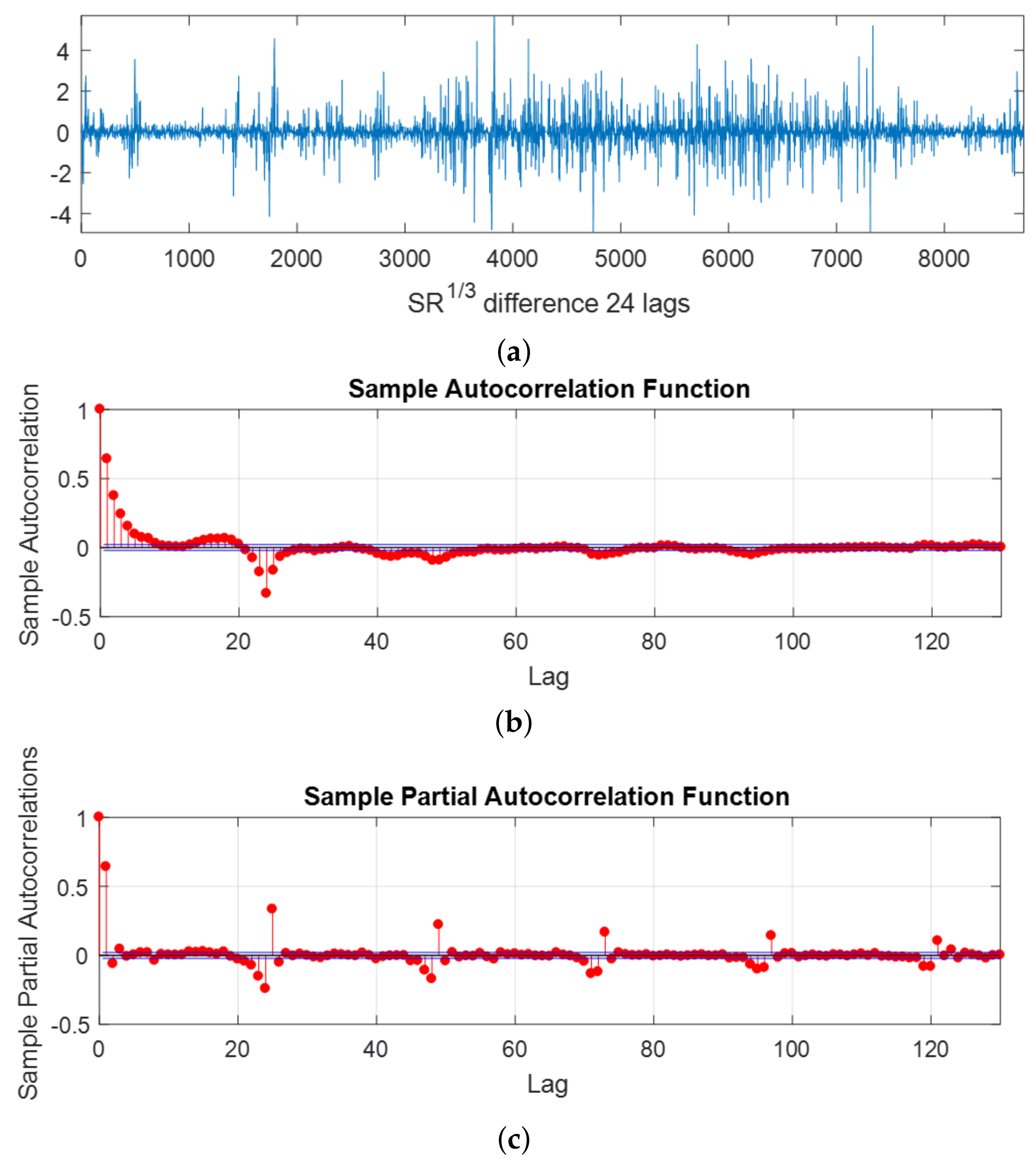
First, the variance and the mean were stabilized through the cubic root of the solar radiation, i.e., $Y_t=S{R}^{1/3}$. Then, it was differentiated using 24 lags, as $d{Y}_t=(1-B^{24})Y_t$. Figure 7a shows the transformation of the solar radiation time-series resulting from the application of these operations. After that, the autocorrelation function (ACF) and the partial autocorrelation function (PACF) were obtained from the stabilized solar radiation time-series. Figure 7b shows the sinusoidal behavior of the ACF, which was a clear sign of the presence of seasonality in the SR times-series. At the same time, the PACF displayed peaks every 24 h, which indicated that the time-series presented daily evolution; see Figure 7c. Therefore, the NARX models were tested with different numbers of time lags until reaching 24 lags. The results showed that the best predictions were obtained when 24 lags were used.

4.6. Artificial Neural Network Setup

Figure 8 shows the general flowchart of the input variables’ combinations of the NARX models proposed for the SR forecast at each site; see Table 6, Table 7 and Table 8. For Chihuahua, the architecture of the artificial neural network with all available input variables, i.e., $x\left(t\right)=[SR,T,RH,P]$ and $y\left(t\right)=\left[SR\right]$ as the output variable, is presented in Figure 8a. Figure 8b,c shows how the input variables were previously treated with the collinearity test, resulting in two input vectors built with three variables each. Because the temperature and the pressure were defined as collinear, both variables were separated from the original model, and two new input vectors were generated: in the first one, the temperature was combined with solar radiation and relative humidity, $x\left(t\right)=[SR,RH,T]$; while in the second one, the pressure was combined with solar radiation and relative humidity, $x\left(t\right)=[SR,RH,P]$. In this case, Figure 8d was not used; it was only applicable in the case of Temixco. Finally, Figure 8e shows the performed procedure on the input variables, before applying the NARX model. The four original meteorological variables were treated with the collinearity and the causality tests. Therefore, the inlet vector was reduced from four variables to two variables, namely $x\left(t\right)=[SR,T]$.

Similarly to the Chihuahua case, the NARX model that included all meteorological variables available in the site as inputs is presented in Figure 8a, where $x\left(t\right)=[SR,WS,RH,T,P]$. According to the collinearity tests, the temperature, the relative humidity, and the pressure showed collinearity. Consequently, these variables could not be combined to build the input vectors. Figure 8b–d shows how the input vectors were generated using the collinearity tests, namely $x\left(t\right)=[SR,WS,T]$, $x\left(t\right)=[SR,WS,RH]$, and $x\left(t\right)=[SR,WS,P]$, respectively. Finally, in Figure 8e, the solar radiation and temperature were considered as input variables to the NARX model. This vector was obtained from the application in the collinearity and causality tests. As can be seen, the results of the collinearity and the causality tests were not included for the cases $V_3=[SR,WS,RH]$ and $V_4=[SR,WS,P]$; this was because, when applying the causality test to these cases, the results did not suggested any change. Nevertheless, the only change observed occurred when the causality test was applied to $V_2=[SR,WS,T]$; where, according to the causality test, WS did not cause SR. Therefore, in this particular case, the input vector was composed as $x\left(t\right)=[SR,T]$.

According to the collinearity test, the only variable that presented collinearity was the temperature. Therefore, there was no restriction in combining T with another variable. Figure 8a shows the NARX architecture using all available variables for the site of Zacatecas, that is $x\left(t\right)=[SR,T,RH,WS]$. Figure 8b,c shows the inlet vectors resulting from the collinearity tests, namely $x\left(y\right)=[SR,T,RH]$ and $x\left(y\right)=[SR,T,WS]$, respectively. When applying the causality tests to the combination of variables $[SR,T,RH]$, the results indicated that the three variables should be used for the SR prediction. Nevertheless, when applying the causality test to $[SR,T,WS]$, the results indicated that WS did not cause SR, that is WS should not be used for the SR forecast. In Figure 8d, the architecture used for the forecast of solar radiation can be seen, which only had SR and T as input variables.

In all cases, the number of neurons used in the hidden layer of the NARX models was 10. The number of lags was obtained using the autocorrelation function and the partial autocorrelation function. The Levenberg–Marquardt algorithm was used as the training algorithm.

5. Results and Discussions

The results were obtained using two specialized software packages: EViews 9.0 [30] and MATLAB 2015a [31]. The first was used to perform the cointegration tests thanks to its versatility and the graphical user interface. The second was used for the normalization of the inlet vectors, the NARX models’ generation, and the collinearity tests.

The forecast results were compared to each other using forecast error measures to verify which configuration of the NARX model had the best performance. Additionally, to have a different comparison pattern, a solar radiation forecast based on the smart persistence model was generated.

5.1. Performance Tests

The results of the performance tests obtained from Equations (18)–(20) are shown in

Table 9. Performance tests for Chihuahua.

Case	Input	Output	Lags	Hidden	MAE	RMSE	${\mathit{Forecast}}_{\mathit{skill}}$
				Neurons	(W/m${}^2$)	(W/m${}^2$)	(%)
1	SR, T, RH, P	SR	24	10	44.1	84.2	−0.4
2	SR, RH, T	SR	24	10	38.2	74.4	11.4
3	SR, RH, P	SR	24	10	39.5	78.2	6.8
4	SR, T	SR	24	10	36.5	74.2	11.5
		Smart Persistence			43.9	83.9	-

,

Table 10. Performance tests for Temixco.

Case	Input	Output	Lags	Hidden	MAE	RMSE	${\mathit{Forecast}}_{\mathit{skill}}$
				Neurons	(W/m${}^2$)	(W/m${}^2$)	(%)
1	SR, WS, RH, T, P	SR	24	10	39.5	79.6	−14.5
2	SR, WS, T	SR	24	10	28.9	58.7	15.5
3	SR, WS, RH	SR	24	10	31.6	61.6	11.3
4	SR, WS, P	SR	24	10	29.7	60.0	13.6
5	SR, T	SR	24	10	29.1	58.6	15.7
		Smart Persistence			32.9	69.5	-

and

Table 11. Performance tests for Zacatecas.

Case	Input	Output	Lags	Hidden	MAE	RMSE	${\mathit{Forecast}}_{\mathit{skill}}$
				Neurons	(W/m${}^2$)	(W/m${}^2$)	(%)
1	SR, T, RH, WS	SR	24	10	50.5	85.7	24.9
2	SR, T, RH	SR	24	10	49.7	84.8	25.6
3	SR, T, WS	SR	24	10	49.6	84.4	26.0
4	SR, T	SR	24	10	46.8	83.0	27.2
		Smart Persistence			67.2	114	-

. Table 9 shows the results obtained for Chihuahua. In the first case, all the available variables in the site were included, this case being where the most significant errors were observed. Once the collinearity and causality techniques were applied, the input vector was reduced to only two variables: SR and T. The collinearity and causality tests restricted the inclusion of every variable that was correlated in the system; for example HR was correlated with T and P; therefore, in our study, only one variable should be incorporated to avoid using redundant information. Finally, it is highlighted that the NARX model that included the collinearity and causality tests showed a better fit than the intelligent persistence model.

Table 10 and Table 11 show the obtained results for Temixco and Zacatecas, respectively. In both cases, the best forecast result was obtained when only SR and T were used to form the input vectors. Therefore, it can be concluded that solar radiation forecasting improved when the collinearity and causality tests were applied to determine the input vector of the NARX model.

It should be noted that, since three study cases were a limited sample to have a conclusive result, the input vectors obtained with the procedure described in this work for other cases could not be SR and T. Thus, the results obtained in this work, concerning the delimitation of the input variables of the NARX models, did not represent a general rule. Furthermore, another determining factor in the conformation of the input vector, other than collinearity and causality tests, was the historical data, on which the training of the forecasting model depended.

Table 9, Table 10 and Table 11 also show the calculation of the forecast skill from Equation (20). It can be observed that the best result was obtained for Zacatecas, then for Temixco, and finally, for Chihuahua. They showed the forecast skill intervals of $27.2\%$, $15.7\%$, and $11.5\%$, respectively.

5.2. Linear Regression Analysis

Linear regression analysis was applied to better visualize forecast accuracy. The results of this analysis are shown in Figure 9, where the x-axis represents the solar radiation forecasting, the y-axis represents the real data, and the blue line is the regression line. This figure shows that the correlation between the real and the predicted data was between $0.94$ and $0.97$, which indicated that the models were very competitive.

For the first two sites, Chihuahua and Temixco, the regression line was almost ${45}^{\circ }$, while the third site had a slightly more pronounced slope. These results indicated that there was a concordance between the SR forecast and the real data. Furthermore, in this figure, it can be appreciated that the data were not very dispersed in any of the graphs, another indication that the forecast results were good.

5.3. NARX Models versus the Smart Persistence Model

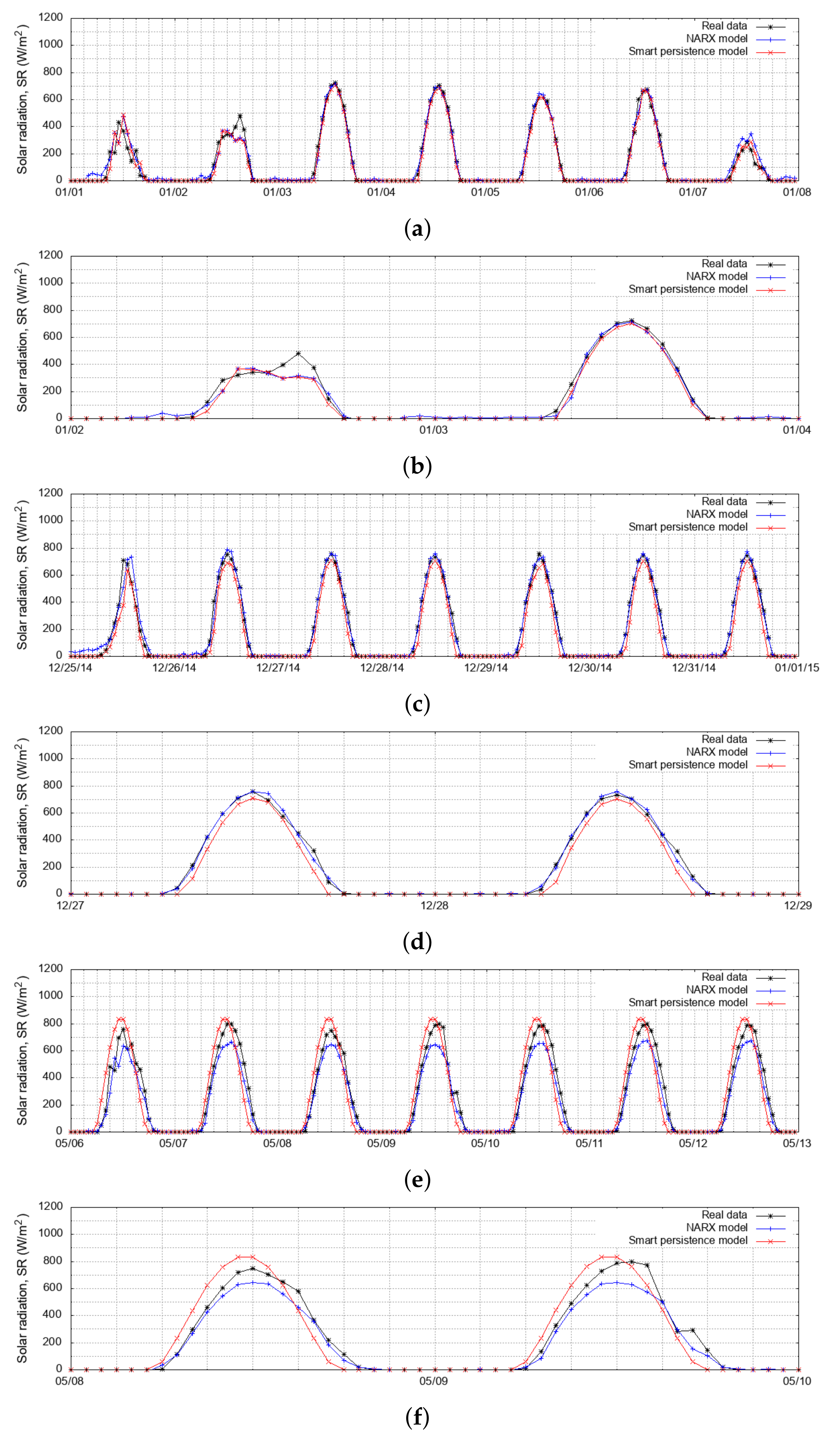
Figure 10 shows a comparison between the solar radiation measured data and the forecasting results obtained from the NARX model and the smart persistence model. Figure 10a presents the results for Chihuahua from 1 January 2015 to 7 January 2015. The RMSE for the NARX model for these seven days was 5.3 W/m${}^2$, while it was 7.3 W/m${}^2$ for the smart persistence model. This chart shows a better fit of the NARX model, especially when the curves did not present a sudden change of direction. When this occurred, both models showed problems fitting to real data; therefore, it was necessary to calculate the prediction error to identify the best-fitting forecast model.

Figure 10b shows the comparison of the last seven days of December 2014 of the solar radiation measured data, NARX model, and smart persistence model for Temixco. The RMSE of the NARX model was 4.5 W/m${}^2$, while 6.1 W/m${}^2$ for the smart persistence model. In this case, both models presented a good performance, with the NARX model being slightly better.

Figure 10c shows the comparison between real and prediction data for 6 May 2007, to 12 May 2007, for the city of Zacatecas. In this case, the RMSE of the NARX model was 7.02 W/m${}^2$, while 10.16 W/m${}^2$ for the smart persistence model. The measured data had an irregular behavior, which caused the NARX model to underestimate the values of SR. In contrast, the smart persistence model overestimated it. Consequently, once again, it was necessary to know the measurement of the prediction error to determine which was the best fit.

Although the graphs did not show much difference between the NARX model and the smart persistence model, the performance tests that were performed for the seven days analyzed in each case indicated that the NARX model was better than the smart persistence model in all cases.

6. Conclusions

Solar radiation is the driving force behind several solar energy devices, such as photovoltaic systems for generating electricity and solar collectors for water heating [1]. Many researchers are interested in proposing and improving forecasting results through new techniques of ANN. In this paper, two tests were applied to three databases to achieve the best variable selection of the input vector of NARX models to improve the SR prediction: the collinearity and causality tests.

In the Chihuahua and Zacatecas cases, there was a clear improvement when applying both tests, nevertheless, in Temixco, there was quite similar performance when the NARX model with $V_2=[SR,T,WS]$ and the NARX model with $V_4=[SR,T]$ were compared. However, the best model used fewer data by eliminating one variable to achieve similar results as the NARX model with vector $V_2$. According to the obtained results, the NARX models that showed the best performance for the solar radiation forecasting one hour ahead were those in which the collinearity and causality tests were applied to determine the proper variables to form the input vectors. Additionally, the input vectors were reduced to use only the significant variables in the forecasting models. The results indicated that, in all studied cases, the solar radiation and temperature were the best combinations of the input variables, which provided better prediction results by using the NARX models.

The prediction results obtained from the NARX models were compared to a benchmark model, the smart persistence model. This model was used to forecast the solar radiation one hour ahead, establishing a relationship between the global solar radiation and solar radiation under clear sky conditions. The solar radiation calculation under clear sky conditions was obtained employing the monthly maximum solar radiation and the monthly maximum extraterrestrial solar radiation. The turbidity coefficient was determined with these monthly values, which is usually obtained through specialized measurement instruments. The solar radiation forecast skill, $\%Forecas{t}_{skill}$, was calculated from the results of the NARX model and the smart persistence model, obtaining $11.5\%$, $15.7\%$, and $27.2\%$ for Chihuahua, Temixco, and Zacatecas, respectively.

The next steps that this research envisages include the expansion of the forecast horizon, i.e., models capable of forecast solar radiation with the least uncertainty for 6, 12, 24, and 48 h ahead. Besides that, numerical models such as the Weather Research and Forecasting (WRF) model could be explored. Additionally, hybrid models involving this kind of numerical model with artificial intelligence and statistical models could be employed, which provide the numerical forecast with the linear and non-linear characteristics of the phenomenon.

References

- Sfetsos, A.; Coonick, A. Univariate and multivariate forecasting of hourly solar radiation with artificial intelligence techniques. Sol. Energy 2000, 68, 169–178. [Google Scholar] [CrossRef]
- Cao, J.; Lin, X. Study of hourly and daily solar irradiation forecast using diagonal recurrent wavelet neural networks. Energy Convers. Manag. 2008, 49, 1396–1406. [Google Scholar] [CrossRef]
- Hocaoǧlu, F.O.; Gerek, Ö.N.; Kurban, M. Hourly solar radiation forecasting using optimal coefficient 2-D linear filters and feed-forward neural networks. Sol. Energy 2008, 82, 714–726. [Google Scholar] [CrossRef]
- Akarslan, E.; Hocaoglu, F.O. A novel adaptive approach for hourly solar radiation forecasting. Renew. Energy 2016, 87, 628–633. [Google Scholar] [CrossRef]
- Boland, J.; David, M.; Lauret, P. Short term solar radiation forecasting: Island versus continental sites. Energy 2016, 113, 186–192. [Google Scholar] [CrossRef]
- Jiménez-Pérez, P.F.; Mora-López, L. Modeling and forecasting hourly global solar radiation using clustering and classification techniques. Sol. Energy 2016, 135, 682–691. [Google Scholar] [CrossRef]
- Martín, L.; Zarzalejo, L.F.; Polo, J.; Navarro, A.; Marchante, R.; Cony, M. Prediction of global solar irradiance based on time series analysis: Application to solar thermal power plants energy production planning. Sol. Energy 2010, 84, 1772–1781. [Google Scholar] [CrossRef]
- Monjoly, S.; André, M.; Calif, R.; Soubdhan, T. Hourly forecasting of global solar radiation based on multiscale decomposition methods: A hybrid approach. Energy 2017, 119, 288–298. [Google Scholar] [CrossRef]
- Azimi, R.; Ghayekhloo, M.; Ghofrani, M. A hybrid method based on a new clustering technique and multilayer perceptron neural networks for hourly solar radiation forecasting. Energy Convers. Manag. 2016, 118, 331–344. [Google Scholar] [CrossRef]
- Benmouiza, K.; Cheknane, A. Forecasting hourly global solar radiation using hybrid k-means and nonlinear autoregressive neural network models. Energy Convers. Manag. 2013, 75, 561–569. [Google Scholar] [CrossRef]
- Chen, C.R.; Kartini, U. k-Nearest Neighbor Neural Network Models for Very Short-Term Global Solar Irradiance Forecasting Based on Meteorological Data. Energies 2017, 10, 186. [Google Scholar] [CrossRef] [Green Version]
- Voyant, C.; Muselli, M.; Paoli, C.; Nivet, M.L. Numerical weather prediction (NWP) and hybrid ARMA/ANN model to predict global radiation. Energy 2012, 39, 341–355. [Google Scholar] [CrossRef] [Green Version]
- Voyant, C.; Muselli, M.; Paoli, C.; Nivet, M.L. Hybrid methodology for hourly global radiation forecasting in Mediterranean area. Renew. Energy 2013, 53, 1–11. [Google Scholar] [CrossRef] [Green Version]
- Ji, W.; Chee, K.C. Prediction of hourly solar radiation using a novel hybrid model of ARMA and TDNN. Sol. Energy 2011, 85, 808–817. [Google Scholar] [CrossRef]
- Renno, C.; Petito, F.; Gatto, A. ANN model for predicting the direct normal irradiance and the global radiation for a solar application to a residential building. J. Clean. Prod. 2016, 135, 1298–1316. [Google Scholar] [CrossRef]
- Kaplanis, S.; Kaplani, E. Stochastic prediction of hourly global solar radiation for Patra, Greece. Appl. Energy 2010, 87, 3748–3758. [Google Scholar] [CrossRef]
- Pandey, P.K.; Soupir, M.L. A new method to estimate average hourly global solar radiation on the horizontal surface. Atmos. Res. 2012, 114–115, 83–90. [Google Scholar] [CrossRef]
- Yang, D.; Jirutitijaroen, P.; Walsh, W.M. Hourly solar irradiance time series forecasting using cloud cover index. Sol. Energy 2012, 86, 3531–3543. [Google Scholar] [CrossRef]
- Wu, J.; Chan, C.K. Prediction of hourly solar radiation with multi-model framework. Energy Convers. Manag. 2013, 76, 347–355. [Google Scholar] [CrossRef]
- Huang, J.; Korolkiewicz, M.; Agrawal, M.; Boland, J. Forecasting solar radiation on an hourly time scale using a Coupled AutoRegressive and Dynamical System (CARDS) model. Sol. Energy 2013, 87, 136–149. [Google Scholar] [CrossRef]
- Hocaoglu, F.O.; Karanfil, F. A time series-based approach for renewable energy modeling. Renew. Sustain. Energy Rev. 2013, 28, 204–214. [Google Scholar] [CrossRef]
- Ahmad, A.; Anderson, T.N.; Lie, T.T. Hourly global solar irradiation forecasting for New Zealand. Sol. Energy 2015, 122, 1398–1408. [Google Scholar] [CrossRef] [Green Version]
- Aguiar, L.M.; Pereira, B.; Lauret, P.; Díaz, F.; David, M. Combining solar irradiance measurements, satellite-derived data and a numerical weather prediction model to improve intra-day solar forecasting. Renew. Energy 2016, 97, 599–610. [Google Scholar] [CrossRef] [Green Version]
- Belsley, D.; Kuh, E.; Welsch, R. Regression Diagnostics: Identifying Influential Data and Sources of Collinearity; Wiley Series in Probability and Statistics; John Wiley & Sons: Hoboken, NJ, USA, 1980. [Google Scholar] [CrossRef]
- Gujarati, D.N.; Porter, D.C. Basic Econometrics, 5th ed.; McGraw-Hill Publishing: New York, NY, USA, 2013. [Google Scholar]
- Haykin, S. Neural Networks a Comprehensive Foundation, 2nd ed.; Pearson Prentice Hall: Upper Saddle River, NJ, USA, 2004; Volume 1, p. 823. [Google Scholar]
- Chu, Y.; Pedro, H.T.C.; Coimbra, C.F.M. Hybrid intra-hour DNI forecasts with sky image processing enhanced by stochastic learning. Sol. Energy 2013, 98, 592–603. [Google Scholar] [CrossRef]
- Tiwari, G.N.; Tiwari, A.; Shyam. Handbook of Solar Energy. Theory, Analysis and Applications, 1st ed.; Springer: Singapore, 2016. [Google Scholar] [CrossRef] [Green Version]
- Behar, O.; Khellaf, A.; Mohammedi, K. Comparison of solar radiation models and their validation under Algerian climate—The case of direct irradiance. Energy Convers. Manag. 2015, 98, 236–251. [Google Scholar] [CrossRef]
- EViews. EViews 9 Student/Lite Version; IHS Global Inc.: Irvine, CA, USA, 2015. [Google Scholar]
- Beale, M.H.; Hagan, M.T.; Demuth, H.B. Neural Network Toolbox ™ User’ s Guide R 2013b; The MathWorks Inc.: Natick, MA, USA, 2013. [Google Scholar]
Figure 1.
Weather map of Mexico (source: Instituto Nacional de Estadística, Geografía e Informática).
Figure 2.
Proposed NARX model: (a) Nonlinear autoregressive neural network with exogenous inputs. (b) Multilayer perceptron with one hidden layer [26].
Figure 3.
Solar radiation under clear sky conditions (): (a) Chihuahua: 1 January to 31 December 2015; (b) Chihuahua: 1–31 January 2015; (c) Temixco: 1 January to 31 December 2014; (d) Temixco: 1–31 January 2014; (e) Zacatecas: 1 January to 31 December 2007; and (f) Zacatecas: 1–31 January 2007.
Figure 4.
Results of the collinearity tests: (a) Chihuahua, (b) Temixco, and (c) Zacatecas.
Figure 5.
Nonlinear autoregressive exogenous model: (a) Main flow chart. (b) Variables’ normalization subprocess.
Figure 6.
NARX model including collinearity and the Engle–Granger test.
Figure 7.
Autocorrelation functions analysis: (a) Transformation of the original time-series. (b) Autocorrelation function. (c) Partial autocorrelation function.
Figure 8.
General architecture of the NARX models: (a) using all available variables, (b) obtained from the collinearity test application, (c) obtained from the collinearity test application, (d) obtained from the collinearity test application (only for the case of Temixco), and (e) or (only for the case of Temixco) obtained from the collinearity and causality tests’ application.
Figure 9.
Linear regression analysis: (a) Chihuahua, (b) Temixco, and (c) Zacatecas.
Figure 10.
Comparison between the forecasting models and measured data: (a) Chihuahua: one week, (b) Chihuahua: two days, (c) Temixco: one week, (d) Temixco: two days, (e) Zacatecas: one week, and (f) Zacatecas: two days.