Article

A Real-Time Dynamic Fuel Cell System Simulation for Model-Based Diagnostics and Control: Validation on Real Driving Data

by
Daniel Ritzberger
1,*,
Christoph Hametner
2 and
Stefan Jakubek
1
1
Institute of Mechanics and Mechatronics, TU-Wien, 1060 Vienna, Austria
2
Christian Doppler Laboratory for Innovative Control and Monitoring of Automotive Powertrain Systems, 1060 Vienna, Austria
*
Author to whom correspondence should be addressed.
Submission received: 29 May 2020 / Revised: 10 June 2020 / Accepted: 12 June 2020 / Published: 17 June 2020
(This article belongs to the Special Issue Polymer Electrolyte Membrane Fuel Cell Systems)

Abstract

:
Fuel cell systems are regarded as a promising candidate in replacing the internal combustion engine as a renewable and emission free alternative in automotive applications. However, the operation of a fuel cell stack fulfilling transient power-demands poses significant challenges. Efficiency is to be maximized while adhering to critical constraints, avoiding adverse operational conditions (fuel starvation, membrane flooding or drying, etc.) and mitigating degradation as to increase the life-time of the stack. Owing to this complexity, advanced model-based diagnostic and control methods are increasingly investigated. In this work, a real time stack model is presented and its experimental parameterization is discussed. Furthermore, the stack model is integrated in a system simulation, where the compressor dynamics, the feedback controls for the hydrogen injection and back-pressure valve actuation, and the purging strategy are considered. The resulting system simulation, driven by the set-point values of the operating strategy is evaluated and validated on experimental data obtained from a fuel cell vehicle during on-road operation. It will be shown how the internal states of the fuel cell simulation evolve during the transient operation of the fuel cell vehicle. The measurement data, for which this analysis is conducted, stem from a fuel cell research and demonstrator vehicle, developed by a consortium of several academic and industrial partners under the lead of AVL List GmbH.

1. Introduction

The paradigm shift in the global energy economy towards sustainable and renewable alternatives has led to an increase in academic and industrial fuel cell activities. The development of fuel cell systems has surpassed the prototype phase as several OEMs already offer fuel cell (FC) vehicles in small series. With the increase of the technological readiness, the requirements imposed on the fuel cell system are becoming more and more stringent. To increase the market penetration and competitiveness, specific costs need to be reduced while durability and efficiency have to be increased [1]. These requirements lead to conflicting goals. For example, it is desired to reduce the capacity of the auxiliary battery, in order to save costs. However, this leads to a more direct and dynamic exposure of the fuel cell system to transient power demands. During these transients, several internal states should be maintained within defined limits so as to prevent the onset of critical operating conditions such as oxygen or hydrogen starvation, excessive membrane humidity cycles, flooding and dry-out [2,3], imposing a significant challenge on any control scheme. This is further aggravated by the fact that the critical internal states of the fuel cell stack cannot be measured directly, or it is just not economically reasonable to do so. To meet these challenging and possibly conflicting goals (i.e., an efficient operation is not necessarily fault tolerant or life-preserving), advanced model-based analysis, diagnostics and control methods [4,5,6] are becoming indispensable.
The intended use of a model determines the trade-off between its complexity and accuracy. For real-time diagnostics and control applications, various fuel cell stack models, which are typically of low spatial dimensionality, were proposed [7,8,9,10,11]. However, the achievable simulation accuracy is not only determined by the model structure, but also by its capability to be parameterized on experimental data. Preliminary studies on dynamic fuel cell stack models were conducted in [7,12]. Therefore, the transient effects during the dynamic, automotive operation are analyzed in simulation. Extensive experimental validation is not provided. A more detailed discussion on the experimental parameterization and validation, using measurements on a single cell, is found in [13]. Therefore, the need for a parametric sensitivity analysis of the model, as a prerequisite for a successful parameterization, is also mentioned. In recent years, the topic of experimental parameterization of fuel cell models gained more attraction. The proposed parameterization schemes mainly revolve around the use of heuristic and gradient free optimization techniques (such as differential evolution, genetic algorithms, particle swarm optimization [14,15,16]), as they tend to be robust for the price of high computational effort and slow convergence. Macroscopic fuel cell system simulations, embedded into a virtual vehicle can be found in [17,18]. For the validation of these macroscopic vehicle models, the simulated vs. measured vehicle velocity is compared, for which a virtual driver (i.e., a feedback control law) is required. It is to be noted that due to this closed loop behaviour of the model, the achieved accuracy in the target velocity profile is substantially influenced by the virtual driver.
In this work, a zero-dimensional, transient fuel cell stack model is presented, striking a reasonable balance between accuracy and computational effort. In addition to the gas-dynamics in cathode and anode, described by the interconnection of zero-dimensional volumes, the diffusion through the gas diffusion layer is considered on the cathode side as well as the transient humidification of the membrane.
For the experimental parameter estimation of the proposed model, a highly efficient parameterization methodology is used. Therefore, the non-linear fuel cell stack model is approximated using multiple local linear models which are obtained via analytic linearization. Due to this, the relation between each local linear model and the parameter vector of the original non-linear model is retained. As such, additional local linear models (and corresponding experiments) can be added to the parameterization in order to improve the estimation accuracy, without introducing additional parameters. After parameterization, the stack model is integrated into a virtual system simulation considering the compressor dynamics, the feedback controllers applied for anode and cathode pressure control and the purging strategy. As such, the virtual fuel cell system is subjected to the same dynamic set point demand trajectories as the real fuel cell vehicle (determined by the operating strategy). The resulting simulation accuracy of the parameterized stack model, embedded into the system simulation is then compared to the real driving data of a fuel cell vehicle during road operation. This demonstrator vehicle (shown in Figure 1) was developed in the KEYTECH4EV project [19] and allows invaluable access to the internal sensor values of the fuel cell system. As such, the validation of the system simulation can be carried out in detail.
The demonstrator vehicle is based on a hybrid VW Passat that was retro-fitted with a fuel cell system (ElringKlinger NM5 stack [20]). System integration and functional operation development was conducted at AVL List Gmbh. The general specifications of the fuel cell demonstrator vehicle can be seen in Table 1. For the measured drive cycle of the vehicle, the internal states of the stack simulation are investigated, giving invaluable information from the fuel cell stack during the transient operation. For example, it is analyzed how nitrogen is accumulated in the anode or how the membrane humidity is affected during the transient vehicle operation. After evaluation of the system simulation with real driving data, the paper gives an open ended discussion of possible use-cases and potential improvements in fuel cell system control and diagnosis, based on the premise of such a real-time capable model.
The remaining paper is organized as follows: In Section 2, the zero-dimensional, dynamic and real-time computable fuel cell stack model is presented. The parameterization methodology, based on the analytic linearization of the stack model, is briefly reviewed. As the linearization requires continuous differentiability, suitable approximations for the discontinuous switching and saturation nonlinearities are introduced. In Section 3, the fuel cell stack model is integrated into the system simulation, which is then driven by the same set-point values determined by the operating strategy of the vehicle. The resulting accuracy of the system simulation and the internal states of the fuel cell stack for the measured drive-cycle of the vehicle are presented in Section 4. A brief discussion on potential use-cases of such a system simulation, outlining future work is given in Section 5.

2. Fuel Cell Stack Model

This section focuses on the derivation of the fuel cell stack model, used in the system simulation. In order to meet the requirement of real-time computability, a zero-dimensional modeling approach is used (the model schematic can be seen in Figure 2). The cathode (ca) and anode (an) pathways are divided into three manifolds: supply manifold (SM), center manifold (CM), and exit manifold (EM). The center manifold is thought of as the lumped volume of the FC stack anode and cathode respectively. Supply and exit manifold represent the auxiliary volumes in front and after the stack, which is also where the sensors (mass flow, pressure, humidity) reside. On the cathode side, transient diffusion of species through the gas diffusion layer (GDL) to the catalyst layer (CL) is considered, leading to an additional volume, whose inflows are determined by Fick’s diffusion. On the cathode side, the consumption of oxygen and the generation of product water is carried out in the catalyst layer manifold, whereas on the anode side the mass fluxes due to reaction and crossover of species are directly coupled to the center manifold. A transient phase change from water vapor to liquid water is considered when the water vapor partial pressure exceeds the saturation pressure.

2.1. Derivation of Model Equations

The dynamics of the considered species
i { H 2 , O 2 , N 2 , H 2 O vap }
are then governed by balancing the masses for the interconnected volumes
v { SMan , CMan , EMan , SMca , CMca , EMca , CLca }
which is formally stated as
d m i , v d t = W i , v , in + W i , v , R + W i , v , out .
Thereby, W i , v , R denotes the manifold-specific source and sink terms (e.g., reaction of hydrogen and oxygen, generation of product water, membrane water transport and nitrogen crossover). A summary of the manifold specific source and sink terms is given in the Appendix A in Table A1. The mass flows between manifolds are described by a linear nozzle equation
W i , v , in = y i , v 1 k v Δ p v ,
where k v denotes the linear nozzle coefficient and Δ p v the pressure difference with respect to the previous volume Δ p v = p v 1 p v . The linear nozzle flow Equation (4) can be readily exchanged with the nonlinear nozzle equation [21] to differentiate between choked and non-choked flow conditions. However, owing to the already existing model simplifications, and adhering to a parsimonious modeling principle, the linear flow equations are used in this work. Furthermore, it is assumed that the mass fractions of the in-flowing species y i , v 1 are given by the mass fractions of species in the previous manifold. Also due to consistency, it follows that W i , v , in = W i , v 1 , out . Note that for the catalyst layer manifold W i , C L c a , in = W i , C L c a , out = 0 . This corresponds to the assumption that the flow from center manifold to the catalyst layer is governed by diffusion and convective mass transport through the GDL is neglected [22,23]. The supply manifold in-flows W i , S M a n / S M c a , in can be calculated from the (measured) overall mass flows W S M a n / S M c a , in and the relative humidities ϕ S M a n / S M c a , in . The actuation of the back-pressure valve on cathode and purge valve on the anode are described by a time-varying nozzle coefficient
k E M a n / E M c a ( t ) = α E M a n / E M c a ( t ) k ˜ E M a n / E M c a ,
where k ˜ E M a n / E M c a denotes the nominal nozzle coefficient and α E M a n / E M c a ( t ) 0 , 1 the actuation signal of the valve.
The mass of species i in manifold v can be related to its partial pressures via the ideal gas law [24],
p i , v = m i , v V v R i T ,
where R i denotes the specific gas constant of species i, V v the volume of manifold v, and T the temperature, which is assumed to be uniform in the stack. The overall pressure in volume v is then given by
p v = i p i , v .
Note that when there are no species-specific source and sinks terms in a manifold (as in the supply and exit manifolds), the individual balancing of species is not necessary, as the resulting differential equations for each species will be linear dependent. In order to arrive at a minimal realization of the model (i.e., minimum number of individual states in the model) the overall mass or pressure can be balanced instead.
When the water vapor partial pressure p H 2 O vap , v in volume v exceeds the saturation pressure (which is assumed to be a function of temperature p sat ( T ) [24]) liquid water starts to condense. To capture this effect, transient phase change relations are considered [25,26,27]:
A mass balance for liquid water yields
d m H 2 O liq , v d t = W phase , v ,
with the phase change rate defined as
W phase , v = k ˜ cond ( t ) p H 2 O vap , v p sat ( T ) , if p vap ca > p sat ( T ) k ˜ evap ( t ) p H 2 O vap , v p sat ( T ) , otherwise .
Therefore, k ˜ cond ( t ) and k ˜ evap ( t ) denote the time-varying, lumped condensation and evaporation rate constants. A detailed discussion and exact numerical expressions thereof can be found in [27]. Note that any transport mechanisms of liquid water are currently neglected. As such, liquid water remains in its respective volume where it has condensed until it evaporates again.
The recirculation from the anode exit manifold to supply manifold is considered via an additional massflow W an , reci which is assumed to be known.
The transient wetting and drying of the membrane is modeled as a simple first order system with a time constant τ m , using the average water activity of cathode and anode as an input:
a ˙ m = 1 τ m a m + a CLca + a CMan 2 ,
with
a k = p H 2 O vap , k p sat ( T ) k { CLca , CMan } .
The dynamic membrane water activity a m is used to determin the ohmic resistance, the electro-osmotic drag and back diffusion coefficient [28]. The electrochemical model used in this work, coupling the thermodynamic quantities (partial pressures of species, membrane humidity), current and voltage, assumed to be static. This corresponds with to the fact that the time constants of the electrochemical reactions are several orders of magnitude faster then the time-constants associated with the convective and diffusive transport of species [29]. The electrochemical model is described and discussed in detail in [30].
Aggregating all differential equations describing the fuel cell stack leads to a highly non-linear state-space model of the form
x ˙ = f ( x , u , θ ) ,
y = g ( x , u , θ ) .
In the remainder of this work, bold lower case letters are used to indicate a vector and bold upper case letters indicate a matrix. The input u and state x vector defined as
u = W SMan , in W SMca , in ϕ SMan , in α EMan α EMca T I , x = p SMca m O 2 , CMca m N 2 , CMca m H 2 O vap , CMca m O 2 , CLca m N 2 , CLca m H 2 O vap , CLca m H 2 O liq , CLca p EMca p SMan m H 2 , CMan m N 2 , CMan m H 2 O vap , CMan m H 2 O liq , CMan p EMan a m .
The output vector y is specific to the application of the model. For the task of model parameterization, the output vector is defined by the available measurements, whereas for the application in fault diagnostic- and model-based control, all internal states and derived quantities (e.g., partial pressures/concentrations of species, membrane humidity, accumulated nitrogen in anode, stack efficiency etc.) can be accessed.

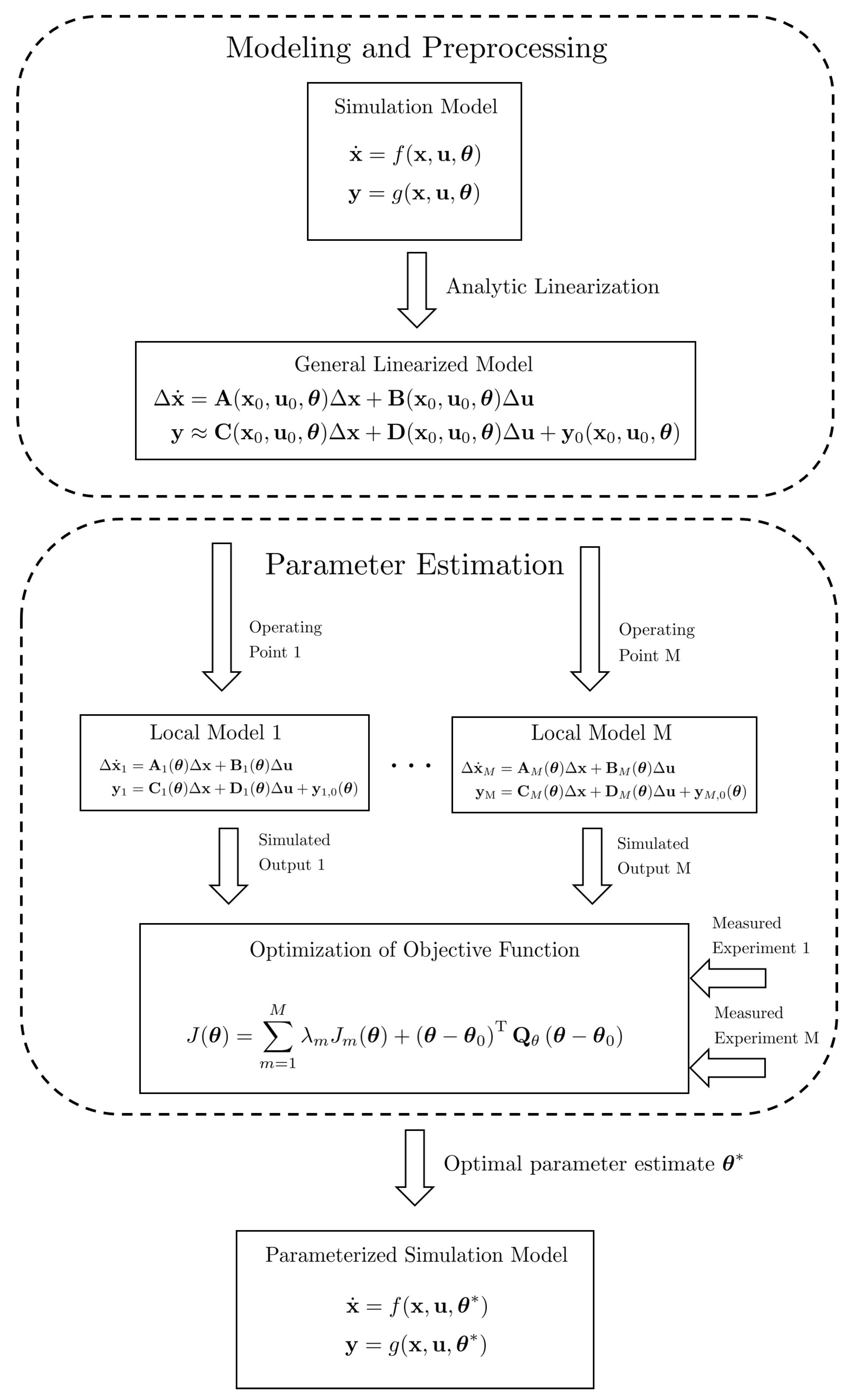
2.2. Model Parameterization

So far, the structure of the fuel cell stack model was defined and derived. However, one important aspect is still to be discussed. In order to achieve a suitable degree of accuracy of the simulation model, the parameteres θ in (12) and (13) have to correspond to the actual fuel cell system under investigation. Some parameters might be derived from fundamental constants, geometric considerations or expert knowledge (with varying levels of accuracy). However in the general case, they have to be inferred from the available experimental data; a scientific discipline also known as system identification [31].
One often encountered methodology in order to parameterize such a non-linear state space models with a fixed model structured (also known as grey-box model estimation [32,33]) is based on the minimization of the model output error. However, for the non-linear fuel cell stack model, this was found to be computationally very expensive. Additionally, unfavourable model properties, such as numerical stiffness and discontinuouties, can cause convergence issues. In order to alleviate these issues, a parameterization workflow, based on the simultaneous estimation of multiple local linear models, obtained via analytic linearization, is used.
For the sake of completeness, the model estimation via minimization of the output error, its issues and difficulties, and the parameterization methodology based on simultaneous identification of multiple local linear models are briefly reviewed:
A suitable scalar objective function, based on the output error between simulation model and obtained measurements is given by
J ( θ ) = 1 N k = 1 N y ( θ , k ) y ^ ( k ) T Q y y ( θ , k ) y ^ ( k ) Weighted output error + θ θ 0 T Q θ θ θ 0 Regularization .
Therefore, y ( θ , k ) , denotes the simulated output (with respect to the parameter vector θ ) at a discrete time instance k ( t = Δ t k , with Δ t being the sampling time) and y ^ ( k ) the corresponding measured output. The matrix Q y is used to weight the errors of different outputs with respect to each other. The second term in (15) is used to penalize the deviation of the parameters with respect to the initial parameter. One the one-hand, this is motivated by the fact that certain parameters may be known to some extent (expert-knowledge) with varying levels of confidence. On the other hand, introducing the second term leads to a regularization of the optimization problem.
An optimal parameter estimate with respect to the objective function (15) is then formally stated as
θ ^ * = arg min θ J ( θ ) .
An analytic solution for θ ^ * is in general not obtainable due to the complexity of the optimization problem. The optimal solution is therefore typically approximated using various iterative, numerical optimization algorithms. For the parameterization of the fuel cell stack model, the following issues can arise when trying to numerically solve the optimization problem:
  • The applied ordinary differential equation solver fails to provide a solution of the simulated output y ( θ , k ) (e.g., due to numerical stiffness or improper parameter values during the optimization). As a result, the objective function (15) cannot be evaluated and the parameterizaton task fails.
  • The optimization algorithm does not converge to a suitable solution. A restart of the optimization with different solvers, solver settings and weightings in the objective function is required.
  • The experimental data is not informative enough or conversely, all desired parameters cannot be uniquely determined from the experimental data due (e.g., due to insufficient excitations, sensors or measurement errors).
To alleviate these issues, a parameter estimation methodology, based on analytically derived local linear models, is proposed. At its core, it is based on the following substitution:
Instead of simulating the non-linear model, the model output y is approximated by a local linear model
Δ x ˙ = A ( θ ) Δ x + B ( θ ) Δ u ,
y y lin = C ( θ ) Δ x + D ( θ ) Δ u + y 0 ( θ ) .
where the local inputs Δ u = u u ^ 0 and local states Δ x = x lin x 0 ( θ ) are referenced with respect to a specific steady state operating point. The system matrices are then defined as,
A ( θ ) = f ( x , u , θ ) x x 0 ( θ ) , u ^ 0
B ( θ ) = f ( x , u , θ ) u x 0 ( θ ) , u ^ 0
C ( θ ) = g ( x , u , θ ) x x 0 ( θ ) , u ^ 0
D ( θ ) = g ( x , u , θ ) u x 0 ( θ ) , u ^ 0 .
One key aspect that should be clarified is how to evaluate the partial derivatives in (19)–(22). While a numeric approximation via finite differences is easily obtainable, it bears the distinct disadvantage that the functional relation of the original model parameters to the linear model is thereby lost. This effectively means that during the optimization the numeric linearization would be needed to be carried out at each iteration. On the other hand, when evaluating the partial derivatives analytically, symbolic expressions of the linear system matrices are obtained where the functional dependency on the model parameters is retained. The analytic evaluation of the partial derivatives is done once in a pre-processing step of the model and stored for later use during the optimization. In order for the analytic linearization to succeed, the model needs to be continuously differentiatable. A more detailed discussion about this can be found below in Section 2.3.
When using multiple experiments and corresponding multiple linear models for the parameter estimation, the objective function (15) is adapted to
J ( θ ) = m = 1 M λ m J m ( θ ) + θ θ 0 T Q θ θ θ 0 ,
where
J m = 1 N m k = 1 N m y lin , m ( θ , k ) y ^ ( k ) T Q y y lin , m ( θ , k ) y ^ ( k )
denotes the model output error of the m-th linear model and λ m a corresponding weight. Note that this approach is similar to the system identification via local linear model networks [34], but with the main difference that with the present approach the structure of the local linear models is determined from a physical non-linear model via analytic linearization. Due to this analytic linearization, each local linear model still depends on the original physical parameter vector of the non-linear model. Thus, adding additional experiments and local models to the estimation does not increase the parameter space (as it would be the case for traditional local linear model networks, where each local model is depending on its own parameters [35]).
Note that in order to accommodate the assumption of linearity, the experiments carried out on the fuel cell stack have to be conducted accordingly. This effectively means that instead of having an experiment throughout the whole operating region of the stack (which would be desired for the estimation of the non-linear model) the experimental region of interest is split into several local experiments at defined operating points with a reduced amplitude of excitation. As an added benefit, carrying out local experiments on the fuel cell stack with reduced amplitudes of excitation is less straining and more compliant to operational and safety limitations of a testbed. The parameterization scheme based on the analytic linearization and simultaneous estimation of multiple local linear models is graphically summarized in Figure A1 in the Appendix A. As a main advantage for this method, it was observed that a significant increase in computational efficiency (three orders of magnitude) can be obtained for the parameterization of the proposed fuel cell stack model, as opposed to the minimization of the output error of the non-linear model. This can be mainly attributed to the numerical efficiency of linear ordinary differential equation solvers. Additionally, for linear models, unfavourable model properties such as instability or unreasonable stiffness (which could arise from unsuitable parameter values during optimization and can lead to a termination of the optimization) can be a-priori detected via an eigenvalue analysis and penalized or disregarded in the optimization.

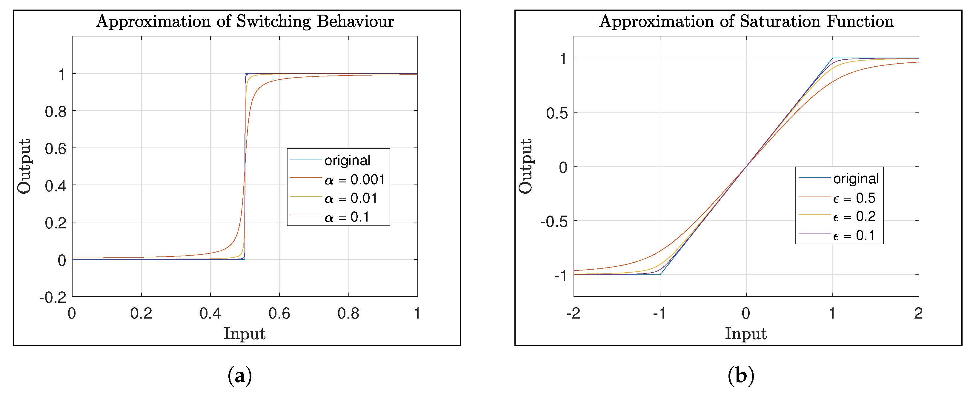
2.3. Approximating Model Discontinuities

To determine the system matrices (19)–(22) analytically, several computer algebra packages are readily available. In the present work MATLABs symbolic math toolbox [36] was used. To ensure that the analytic evaluation of the partial derivatives is successfull, the right-hand-side functions of the non-linear model (12) and (13) need to be continuously differentiatable. However, when modeling the dynamic behaviour fuel cell stack, model discontinuities arise from physical considerations and are required in order to accurately reproduce the behaviour of the stack. One example is the condensation of liquid water: If the partial pressure of water vapor is greater than the saturation pressure, liquid water starts to condense and vice versa. This verbally described If.. Then.. rule correspondonds to a discontinuous switching behaviour of the model. Another example is the saturation function. Masses and pressure cannot become negative. Yet, when simulating a shut-down of the fuel cell stack where the cathode is closed off and the remaining oxygen is being consumed by a small current, neglecting the saturation of masses will lead to a negative oxygen mass in the simulation and the subsequent implausible behaviour of the model.
To still capture these effects while still complying to the requirement of continuous differentiatability, the model discontinuities need to be sufficiently approximated by smooth functions. For the approximation of the switching behaviour,
h ( x ) = a ( x ) , if x x switch b ( x ) , otherwise ,
the following sigmoid activation function
H ( x ) = 1 π atan ( α ( x x switch ) ) + 0.5 ,
can be used. The switching bevahiour is then approximated by
h ( x ) = ( 1 H ( x ) ) a ( x ) + H ( x ) b ( x ) .
The transition coefficient α can then be used to tune the sharpness of the transition area.
A saturation non-linearity with a unitary gain and a lower and upper limit of X min and X max respectively is given by the following exact equation:
y ( x ) = 1 2 ( X min + X max + | x X min | | x X max | ) .
To achieve higher order differentiatability, the absolut value can be approximated using
| z | z 2 + ϵ 2 ,
where ϵ is again a scalar tuning factor. In Figure 3, the switching and saturation function and its smooth approximations for different values of the tuning factors can be seen.
In replacing all discontinuities with appropriate approximations, continuous differentiatability can be ensured. Note that continuous differentiatability is not only required by the parameterization scheme. It also a huge generel advantage, as it enables the use many state-of-the-art nonlinear control and state-estimation schemes based on successive linearization (such as the extended Kalman filter).

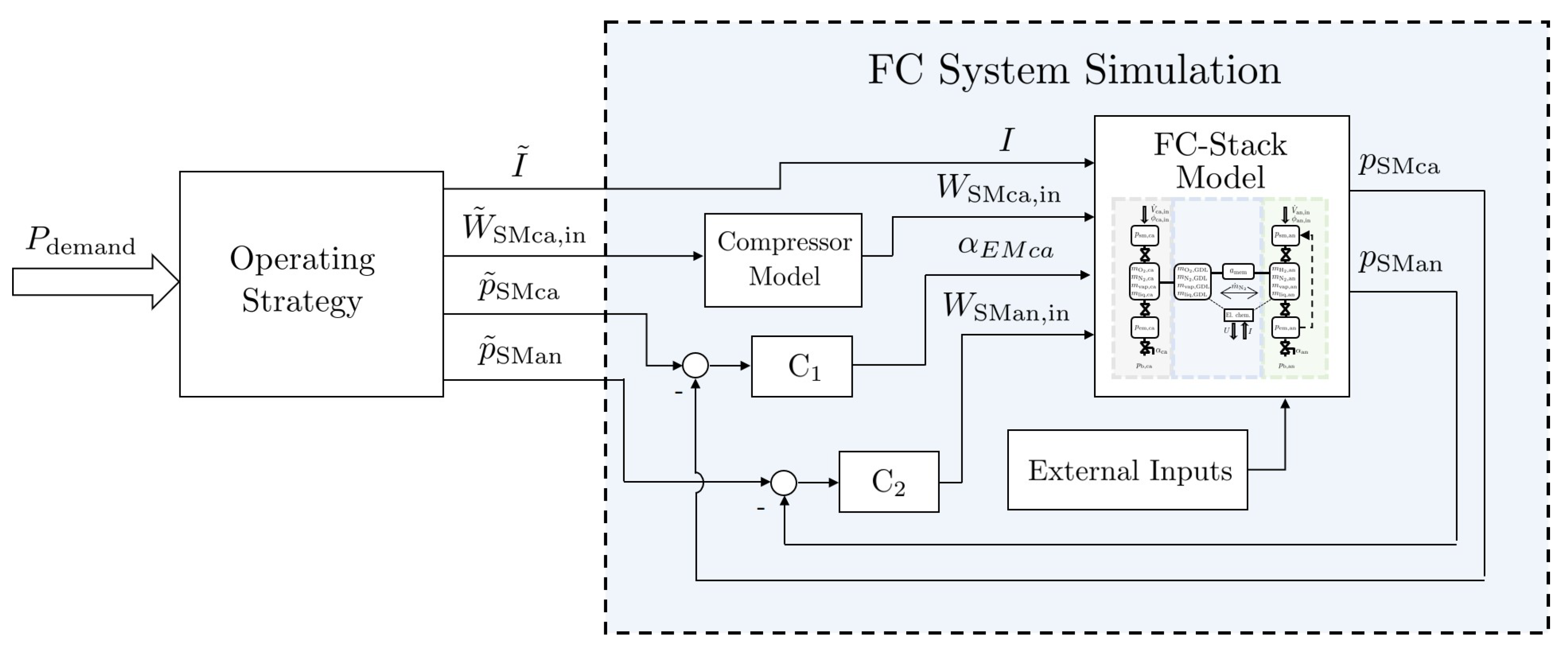
3. Fuel Cell System Simulation

In the previous sections, the isolated fuel cell stack model and its experimental parameterization was presented. In this section, it will be discussed how the stack model is integrated into fuel cell system simulation. In a first step, the system boundaries and the intended use-case of the system simulation need to decided, as this gives an indication about the required modeling depth of auxiliary components in the model. As an example, lets consider the air supply on the cathode. Assuming that the compressor is already suitably controlled, the relation between demanded air mass-flow W ˜ SMca , in and actual mass-flow W SMca , in can be, in its simplest form, considered as a first order system
W SMca , in = 1 1 + τ comp s W ˜ SMca , in ,
where τ comp denotes the response time of the controlled compressor and s the complex valued laplace variable. Therefore, the rotational dynamics and the compressor controls are all lumped together into a single time constant. When investigating competing operating strategies, a simple approach like this might already be sufficient in order to derive dynamic requirements on the compressor with respect to the chosen operating strategy. However, it is obvious that no statements can be made about, for example, the energy consumption of the compressor or if the chosen compressor type is suitable at all. In such a case a more detailed model as in [37] is required. The intended use of the system simulation in the context of this work is as a virtual sensor for fault detection, i.e it is desired to get on-line insights regarding the internal states of the fuel cell stack during the dynamic operation of the vehicle. For this reason, the modeling depth with regard to auxiliary components is relatively shallow. Or rather, the simplest models were ought to be found while still maintaining the integrity of the intended use.
The system simulation setup can be seen in Figure 4. When the driver presses the acceleration pedal, a power demand for propulsion of the vehicle is generated. This power request is divided by the power split strategy into a power demand for the traction battery and a power demand for the fuel cell system. The current power demand P demand is further converted by the vehicle operation strategy into set-points, namely:
  • Stack Current I ˜ ,
  • Cathode inlet air flow W ˜ SMca , in ,
  • Cathode supply manifold pressure p ˜ SMca ,
  • Anode supply manifold pressure p ˜ SMan .
For the stack current I, it is assumed that the power electronics and controls are sufficiently fast such that no additional dynamics have to be considered and the demanded stack current I ˜ is used in the stack simulation. The demanded air massflow W ˜ SMca , in is filtered using a simple first order system as described above. In order to ensure that the demanded supply manifold pressures p ˜ SMca and p ˜ SMan are met, a simplified control scheme based on the real vehicle, was implemented. A feedback controller is used to actuate the back-pressure valve of the cathode, whose position is saturated between [0,1]. In order to fulfill the set-point pressure in the anode, a second feedback controller is implemented, regulating the hydrogen inflow from the tank.
Note that an increase in anodic pressure is implemented straight-forward via the inflow from the tank; however, the rate of decrease of anodic pressure is limited by the consumption of hydrogen, gas crossover and leakages.
A coulomb counting purge strategy was implemented with a valve opening time of 0.3 s. In the demonstrator vehicle, the injection of hydrogen and the anode off-gas recirculation is realized via an ejector/injector unit where the inflow rate (and recirculation rate) is actuated via a pulse-width modulation (PWM) of the injector valve. A control oriented model of an ejector/injector unit can be found in [38,39]; however during simulation it was observed that the high frequency fluctuations (15 Hz) caused by the PWM of the injector valve has drastic negative effects on the computational efficiency of the simulation, while simultaneously causing negligible ripples in pressure. The hydrogen inflow valve is therefore continuously operated in simulation. Additional external inputs used in the system simulation are for example the uniform stack temperature, relative humidity of in-flowing air and the atmospheric pressure.
Note that for a stand-alone simulation of the fuel cell stack, it is not advised to use the measured hydrogen flow as an input to the simulation due to the following reason: When the purge valve is closed, the anode pressure dynamics exhibit an integrating behaviour with respect to the massflow. Since the measured hydrogen massflow (originating from a closed control loop) will be, at least to some extent, subjected to measurement noise or bias the resulting simulated anode pressure will exhibit a random walk or a continuous drift due to the integration of measurement errors. Therefore, either the supply manifold pressure or, as in the real system, a massflow originating from a closed loop control scheme should be used.

4. Results

In this section, the accuracy of the fuel cell system simulation is analyzed and evaluated. During the operation of the research vehicle on the test circuit, the set-point values for the fuel cell system, which are determined by the operating strategy, were recorded. These set-point values are used as an input to the fuel cell system simulation. The resulting simulation output is then compared to available measurements in the vehicle.

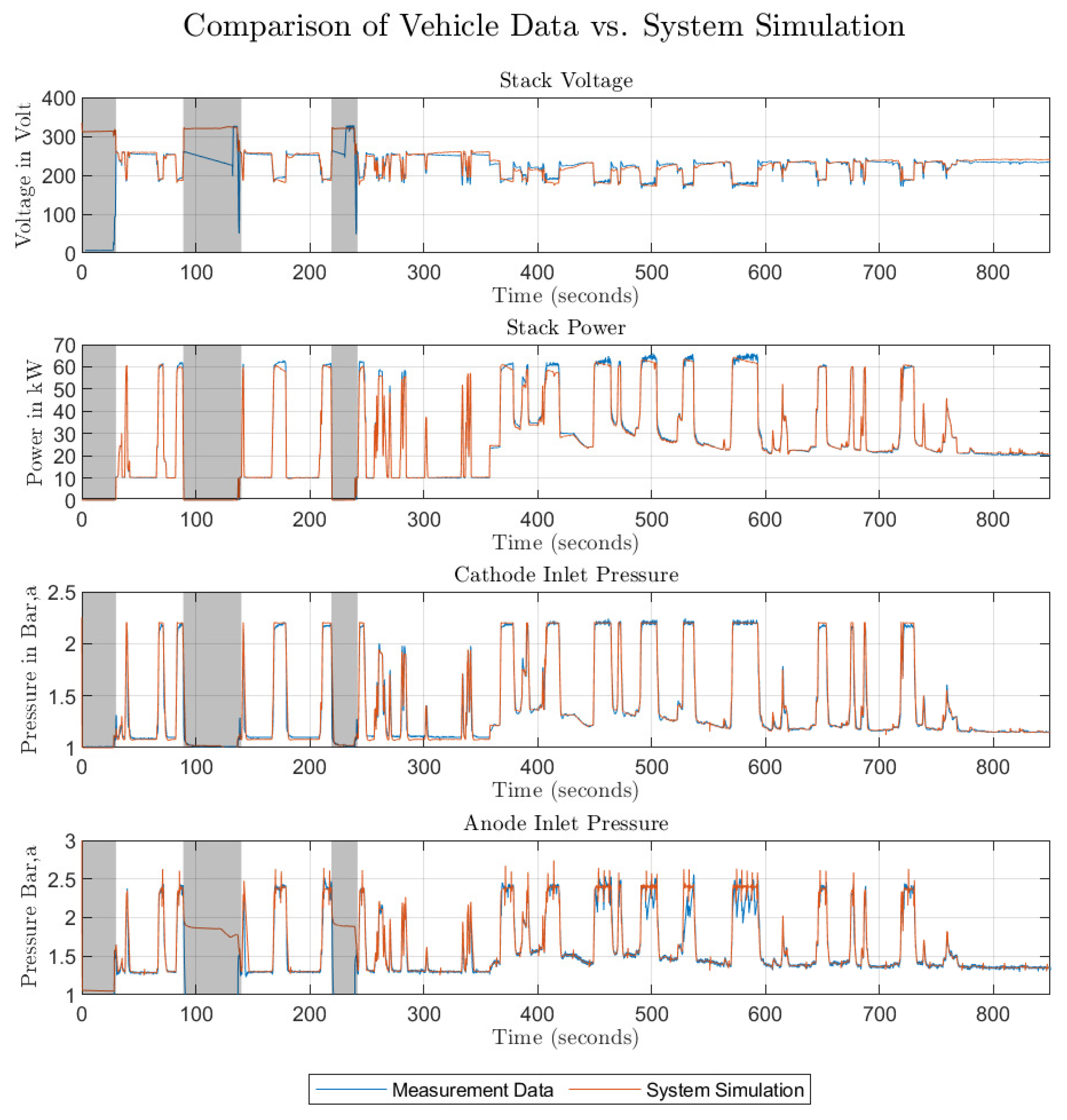
4.1. Validation of the System Simulation

In Figure 5, the outputs of the system simulation, driven by the reference values of the operating strategy, are compared to available measurements in the vehicle. The shaded areas depicted therein mark time intervals during which the vehicle was put into shut-down mode. The associated switching processes of valves as well as in the power electronics during shutdown are not part of the model. As a result, the simulated voltage in the model resorts back to open circuit voltage during shutdown and deviates from the measured voltage of the fuel cell system. During nominal operation of the vehicle however, a remarkable level of agreement between simulated outputs and experimental measurements can be observed. The periodic pressure spikes in the anode, during operation under high pressure, result from the frequent opening of the purge valve. In the current setup, the opening of the purge valve acts as an unknown disturbance. The sudden loss in pressure is then compensated by the feedback controller, regulating the hydrogen inflow, leading to the visible oscillatory behaviour. Substantial improvements could be achieved by using the (known) purge signal in a disturbance rejecting feedforward control scheme.
It is to be noted that no corrections based on measured outputs are taken during the simulation and the results are purely obtained by an independent simulation, driven by the reference-values generated by the operating strategy of the vehicle. The simulation was conducted in MATLAB/Simulink on a single core of personal laptop (CPU: I7-9750H @ 2.60 GHz). The computation time amounted to 81 s for the experiment shown in Figure 5 and is therefore ∼10 times faster then real-time.

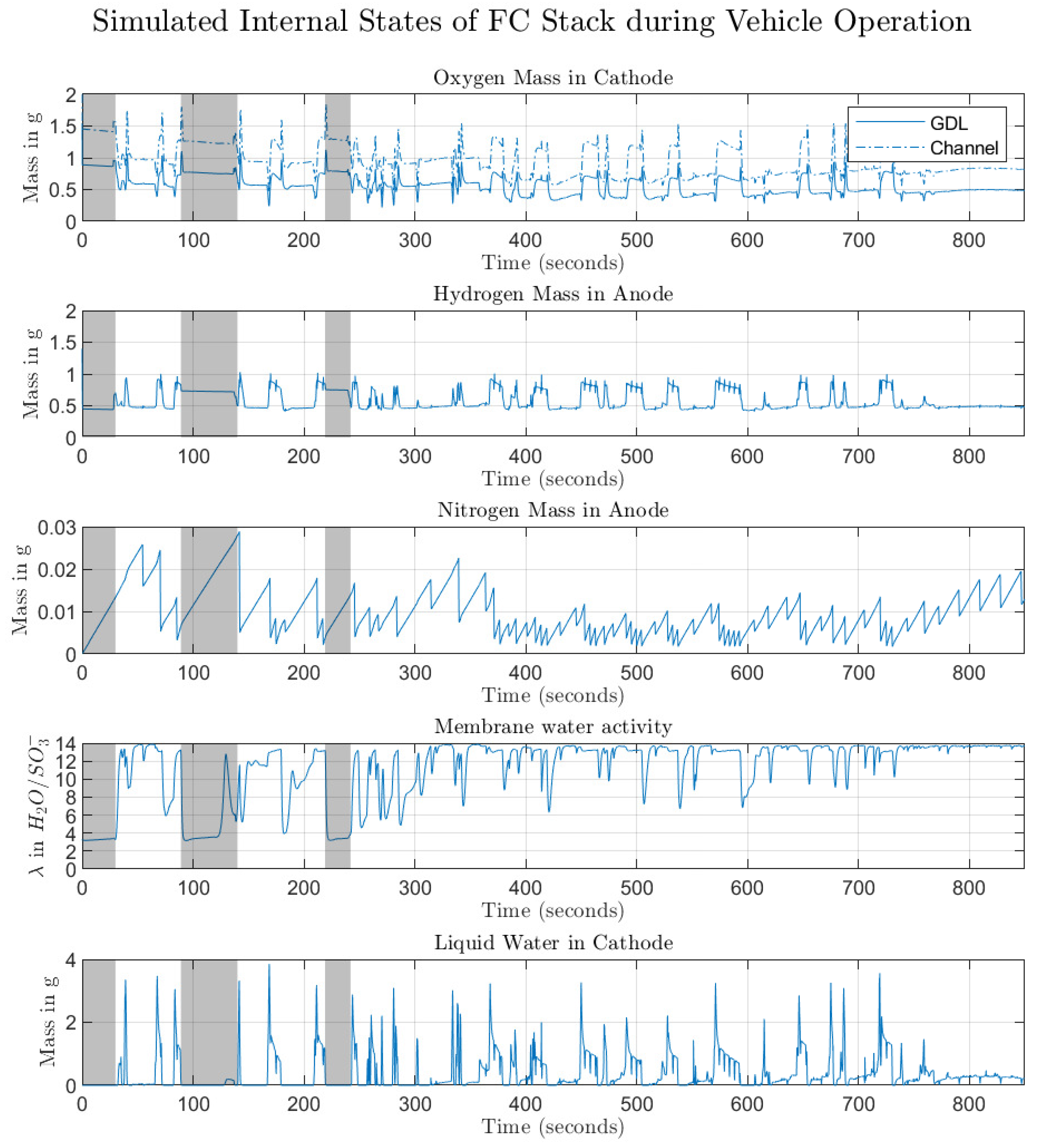
4.2. Investigation of Internal States

In Figure 6, some of the simulated internal states of the fuel cell during the transient operation can be seen. The first two plots show the transient change of oxygen and hydrogen mass in the cathode (Channel and GDL) and anode during the drive cycle. Such real-time signals during operation are an invaluable source of diagnostic information as to prevent fuel starvation. Note that the detection and prevention of fuel starvation is frequently indicated by the stoichiometric ratio [40]. However, under dynamic operating conditions the description using the stoichiometric ratio is somewhat inadequate. For example when determining the stoichiometric ratio for oxygen, the mass flux needed for reaction can be related to the inflow of oxygen into the stack, which is typically measured by a mass flow sensor located between the compressor and the cathode inlet. Under steady state conditions, it is obvious that starvation occurs when the inflowing amount of species is less than the amount required for reaction. However, during transient operation, the use of the stoichiometric ratio, as determined by the amount of inflowing species, may lead to false conclusions, as the internally stored (compressed) oxygen in the cathode and its dynamics and transport processes are thereby completely neglected. The third plot in Figure 6 shows the accumulation of nitrogen in the anode and its rapid discharge due to purging. A coulomb-counting purging strategy was implemented to actuate the purge valve. As hydrogen is ejected during purging, minimum purge action would be desired as to increase the efficiency of the system. With a real-time estimate of the accumulated nitrogen, a threshold purging strategy can be implemented.
The fourth plot in Figure 6 shows the estimated membrane humidity of the fuel cell stack. The overall humidity levels of the membrane tend towards full saturation. However, significant drops in membrane humidity are present during the transient operation of the vehicle. A model-based explanation of this effect is as follows:
During the transient operation, significant changes in anode and cathode pressure of up to 1 bar are encountered (as can be seen in Figure 5). Thus, the water vapor partial pressure in cathode and anode changes proportionally. However, the water vapor saturation pressure (which is a function of temperature) almost stays constant. As such, a decrease in cathode and anode pressure leads to a proportional drop in cathode and anode humidity (e.g., see (11)), thus effecting the membrane humidity. Conversely, when the membrane is fully saturated and the pressure is drastically increased, liquid water start to condense, as can be seen in the fifth plot of Figure 6.

5. Discussion

The results shown above depict a very good agreement between simulated and measured outputs of the fuel cell system over the whole operating range during the transient operation of the vehicle. Also the internal states of the simulation during the transient operation show a plausible behaviour. For a hard validation of internal states however, additional measurements of the fuel cell system on a test-stand would be desired (e.g., high frequency resistance measurements or a dynamic mass spectrometer on the cathode and anode exhaust) which are not available in the vehicle.
Due to the scalability of the zero-dimensional stack model and the proposed robust parameterization scheme, a distinct flexibility in the presented workflow for developing the system simulation is achieved. As such, it can be straight forward adapted to different system architectures and fuel cell stacks. It is obvious that the availability of a real-time computable system simulation enables invaluable possibilities in order to improve the efficiency of a fuel cell stack in a vehicle application. A (non-exhaustive) list is briefly discussed as a reference for future work:
  • State Estimation and Fault Detection: To improve the accuracy with respect to unknown disturbances, measurement noise and emerging faults, the system simulation can be embedded into an observer algorithm to estimate (and correct) the simulation states based on available measurement data. The presented model, as it is continuously differentiatable, is especially suitable for estimation schemes based on successive linearization such as the extended Kalman filter [41]. Having a robust state estimation enables the on-line estimation of hazardous conditions such as fuel starvation, dry-out and flooding and excessive humidity cycles.
  • Model Based Control: The fuel cell system is a strongly coupled multi-input multi-output system for which model-based control methodologies have become indespensible. In a nutshell, the task of the fuel cell system is to provide the required power at the highest possible system efficiency (e.g., considering parasitic consumptions such as the compressor), while taking into account safety and life-time related limitations. The verbal description of the control objective alone points in the direction of optimal control as a suitable candidate. The existence of desired safety-limits, which can be described as constraints either on the inputs, states, or outputs, suggests Model Predictive Control (MPC) [42,43] as a suitable methodology to balance the conflicting goals of life preservation, tracking performance and efficiency maximization. In this sense, the MPC rather takes over the task of planning the operating strategy, which is done on-line together with the a priori information predicted by the real-time model and the a-posteriori correction based on available measurements of the system.
  • Improving the Operating Strategy Even in a non-optimal way it is straight forward to see that the availability of a dynamic fuel cell system simulation enables an engineer to refine the operating strategy with a fraction of the time and costs as opposed to the development at a real test stand. Additionally, all internal states are accessible during the transient operation, which are in general unknown on the real-system.

6. Conclusions

In this work, the performance of a real-time, dynamic fuel cell system simulation is evaluated using experimental data obtained from a fuel cell research vehicle during on-road operation. In order for the simulation to represent the actual system, an efficient model parameterization scheme based on analytic linearization is used. The required continuous differentiatability is ensured by introducing suitable approximations of discontinuities. The fuel cell stack model is then further integrated into a system simulation, which is then compared to the measurements obtained from the vehicle. A remarkable fit of simulated to measured outputs of the fuel cell system was obtained during nominal operation, while being significantly faster then real-time. The simulated transient internal states of the fuel cell stack (such as the masses of oxygen, hydrogen, nitrogen in cathode and anode or the membrane humidity), which are otherwise not measurable, are shown and exhibit plausible behaviour. The presented results highlight the applicability and added value of model-based diagnostic and control methods for the use in fuel cell vehicles. As a main limitation of the present work, it is to be noted that the approach of lumped volumes does not allow for the simulation of spatially resolved information such as pressure and concentration gradients along the channel. Also the effects and transport mechanisms of liquid water can be further refined. In future research the advantages of increased complexity versus their effects on real-time computability needs to be analysed and carefully balanced. Furthermore, the presented parameterization methodology via simultaneous identification via local analytic models could be expanded to accommodate real-time models of higher spatial resolution (1D, quasi-2D).

Author Contributions

D.R. is the main author of the presented work and is responsible for the results shown therein. C.H. provided invaluable feedback during the development and preparation of the manuscript. S.J. contributed excellent scientific supvervision and feedbac throughout this work. All authors have read and agreed to the published version of the manuscript.

Funding

This work has been funded by the Austrian Research Promotion Agency (FFG) in the scope of the “KEYTECH4EV: Development and Demonstration of Key Technologies for Low-cost Electric Vehicle Platforms” project (KR15EF0F12999).

Acknowledgments

The authors would like to acknowledge each industrial and scientific partner, whose efforts were indispensable for the success of the KEYTECH4EV project (in alphabetic order):
  • AVL List GmbH,
  • ElringKlinger AG,
  • HOERBIGER Ventilwerke GmbH & Co Kg,
  • HyCentA Research GmbH,
  • IESTA, Institut für Innovative Energie- und Stoffaustauschsysteme,
  • MAGNA STEYR Engineering AG & Co KG,
  • Technische Universität Graz, Institut für Chemische Verfahrenstechnik und Umwelttechnik,
  • Technische Universität Wien, Institut für Mechanik und Mechatronik.

Conflicts of Interest

The authors declare no conflict of interest.

Abbreviations

The following abbreviations are used in this manuscript:
CLCatalyst layer
CMCenter manifold
EMExit Manifold
FCFuel Cell
GDLGas diffusion layer
MPCModel predictive control
OEMOriginal equipment manufacturer
PEMFCPolymer electrolyte membrane fuel cell
PWMPulse width modulation
SMSupply Manifold

Appendix A. Auxiliary Tables and Figures

Table A1. Individual source terms for the lumped volumes of the fuel cell stack model.
Source TermsDescriptions
W j , CMca , R = W j , GDL
The diffusion of oxygen, nitrogen and water vapor from the center manifold through the GDL to the catalyst layer is described by
W j , GDL = D δ GDL 2 V GDL V CA m j , CMca m j , CLca
Therefore, i CL [ O 2 , N 2 , H 2 O vap ] . D denotes the diffusion coefficient (assumed to be equal for all species) and V GDL the volume of the gas diffusion layer.
W O 2 , CLca , R = W O 2 , GDL W O 2 , react
The massflow of oxygen due to the electrochemical reaction [44] is given by
W O 2 , react = I N cells 4 F M O 2 ,
where I denotes the stack current, N cells the number of cells in the stack, F Faradays constant and M O 2 the molar mass of oxygen.
W N 2 , CLca , R = W N 2 , GDL W N 2 , perm
The permeation of nitrogen from cathode to anode through the membrane is considered via
W N 2 , perm = k perm ( p N 2 , CLca p N 2 , CMan ) ,
with k perm as the permeation coefficient [45].
W H 2 O vap , CLca , R = W H 2 O vap , GDL + W H 2 O vap , react + W H 2 O vap , mem + W phase , CLca
The generation of product water [44] is given by
W H 2 O vap , react = I N cells 2 F M H 2 O vap .
The massflow W H 2 O vap , mem describes the exchange of water vapor through the membrane. Electro-osmotic drag and back-diffusion is considered [28]. W phase , CLca describes the transient, bi-directional phase-change from water vapor to liquid water. The numerical expressions used can be found in [27]
W H 2 , CMan , R = W H 2 , react
The massflow of hydrogen beeing reacted [44] is given by
W H 2 , react = I N cells 2 F M H 2
W N 2 , CMan , R = W N 2 , perm Nitrogen crossover leads to the accumulation of Nitrogen in the anode, which is ejected when the purge valve is actuated.
W H 2 O vap , CMan , R = W H 2 O vap , mem W phase , CMan
The phase change of water vapor to liquid water in the anode center manifold is calculated analogously as for the cathode side.
Figure A1. Workflow of the model parameterization via multiple analytic local linear models.
Energies 13 03148 g0a1

References

  1. Das, V.; Padmanaban, S.; Venkitusamy, K.; Selvamuthukumaran, R.; Blaabjerg, F.; Siano, P. Recent advances and challenges of fuel cell based power system architectures and control—A review. Renew. Sustain. Energy Rev. 2017, 73, 10–18. [Google Scholar] [CrossRef]
  2. Zhao, J.; Li, X. A review of polymer electrolyte membrane fuel cell durability for vehicular applications: Degradation modes and experimental techniques. Energy Convers. Manag. 2019, 199, 112022. [Google Scholar] [CrossRef]
  3. Yousfi-Steiner, N.; Moçotéguy, P.; Candusso, D.; Hissel, D. A review on polymer electrolyte membrane fuel cell catalyst degradation and starvation issues: Causes, consequences and diagnostic for mitigation. J. Power Sources 2009, 194, 130–145. [Google Scholar] [CrossRef]
  4. Petrone, R.; Zheng, Z.; Hissel, D.; Péra, M.C.; Pianese, C.; Sorrentino, M.; Becherif, M.; Yousfi-Steiner, N. A review on model-based diagnosis methodologies for PEMFCs. Int. J. Hydrog. Energy 2013, 38, 7077–7091. [Google Scholar] [CrossRef]
  5. Liu, J.; Luo, W.; Yang, X.; Wu, L. Robust model-based fault diagnosis for PEM fuel cell air-feed system. IEEE Trans. Ind. Electron. 2016, 63, 3261–3270. [Google Scholar] [CrossRef] [Green Version]
  6. Escobet, T.; Feroldi, D.; De Lira, S.; Puig, V.; Quevedo, J.; Riera, J.; Serra, M. Model-based fault diagnosis in PEM fuel cell systems. J. Power Sources 2009, 192, 216–223. [Google Scholar] [CrossRef] [Green Version]
  7. Pukrushpan, J.T.; Stefanopoulou, A.G.; Peng, H. Control of Fuel Cell Power Systems: Principles, Modeling, Analysis and Feedback Design; Springer Science & Business Media: Berlin/Heidelberg, Germany, 2004. [Google Scholar]
  8. Xu, L.; Hu, J.; Cheng, S.; Fang, C.; Li, J.; Ouyang, M.; Lehnert, W. Robust control of internal states in a polymer electrolyte membrane fuel cell air-feed system by considering actuator properties. Int. J. Hydrog. Energy 2017, 42, 13171–13191. [Google Scholar] [CrossRef]
  9. Pilloni, A.; Pisano, A.; Usai, E. Observer-based air excess ratio control of a PEM fuel cell system via high-order sliding mode. IEEE Trans. Ind. Electron. 2015, 62, 5236–5246. [Google Scholar] [CrossRef] [Green Version]
  10. Hong, L.; Chen, J.; Liu, Z.; Huang, L.; Wu, Z. A nonlinear control strategy for fuel delivery in PEM fuel cells considering nitrogen permeation. Int. J. Hydrog. Energy 2017, 42, 1565–1576. [Google Scholar] [CrossRef]
  11. Murschenhofer, D.; Kuzdas, D.; Braun, S.; Jakubek, S. A real-time capable quasi-2D proton exchange membrane fuel cell model. Energy Convers. Manag. 2018, 162, 159–175. [Google Scholar] [CrossRef]
  12. Pathapati, P.; Xue, X.; Tang, J. A new dynamic model for predicting transient phenomena in a PEM fuel cell system. Renew. Energy 2005, 30, 1–22. [Google Scholar] [CrossRef]
  13. Ziogou, C.; Voutetakis, S.; Papadopoulou, S.; Georgiadis, M.C. Modeling, simulation and experimental validation of a PEM fuel cell system. Comput. Chem. Eng. 2011, 35, 1886–1900. [Google Scholar] [CrossRef]
  14. Mo, Z.J.; Zhu, X.J.; Wei, L.Y.; Cao, G.Y. Parameter optimization for a PEMFC model with a hybrid genetic algorithm. Int. J. Energy Res. 2006, 30, 585–597. [Google Scholar] [CrossRef]
  15. Priya, K.; Sathishkumar, K.; Rajasekar, N. A comprehensive review on parameter estimation techniques for Proton Exchange Membrane fuel cell modelling. Renew. Sustain. Energy Rev. 2018, 93, 121–144. [Google Scholar] [CrossRef]
  16. Rajasekar, N.; Jacob, B.; Balasubramanian, K.; Priya, K.; Sangeetha, K.; Babu, T.S. Comparative study of PEM fuel cell parameter extraction using Genetic Algorithm. Ain Shams Eng. J. 2015, 6, 1187–1194. [Google Scholar] [CrossRef] [Green Version]
  17. Kang, S.; Min, K. Dynamic simulation of a fuel cell hybrid vehicle during the federal test procedure-75 driving cycle. Appl. Energy 2016, 161, 181–196. [Google Scholar] [CrossRef]
  18. Boulon, L.; Agbossou, K.; Hissel, D.; Sicard, P.; Bouscayrol, A.; Péra, M.C. A macroscopic PEM fuel cell model including water phenomena for vehicle simulation. Renew. Energy 2012, 46, 81–91. [Google Scholar] [CrossRef]
  19. Keytech4ev Project Homepage. Available online: http://www.iesta.at/keytech4ev/ (accessed on 20 May 2020).
  20. Hemmer, S.; Walters, M.; Tinz, S. Scalable Fuel Cell Systems for Commercial Vehicles. MTZ Worldw. 2019, 80, 64–71. [Google Scholar] [CrossRef]
  21. Zucrow, M.J.; Hoffman, J.D. Gas Dynamics. Volume 2—Multidimensional Flow; Wiley: Hoboken, NJ, USA, 1977. [Google Scholar]
  22. Kulikovsky, A. The voltage–current curve of a polymer electrolyte fuel cell: “Exact” and fitting equations. Electrochem. Commun. 2002, 4, 845–852. [Google Scholar] [CrossRef]
  23. Kulikovsky, A. A physically–based analytical polarization curve of a PEM fuel cell. J. Electrochem. Soc. 2014, 161, F263–F270. [Google Scholar] [CrossRef]
  24. Sonntag, R.E.; Borgnakke, C.; Van Wylen, G.J.; Van Wyk, S. Fundamentals of Thermodynamics; Wiley: New York, NY, USA, 1998; Volume 6. [Google Scholar]
  25. Birgersson, E.; Noponen, M.; Vynnycky, M. Analysis of a two-phase non-isothermal model for a PEFC. J. Electrochem. Soc. 2005, 152, A1021–A1034. [Google Scholar] [CrossRef]
  26. Xu, L.; Fang, C.; Hu, J.; Cheng, S.; Li, J.; Ouyang, M.; Lehnert, W. Parameter extraction and uncertainty analysis of a proton exchange membrane fuel cell system based on Monte Carlo simulation. Int. J. Hydrog. Energy 2017, 42, 2309–2326. [Google Scholar] [CrossRef]
  27. Khajeh-Hosseini-Dalasm, N.; Fushinobu, K.; Okazaki, K. Transient phase change in the cathode side of a PEM fuel cell. J. Electrochem. Soc. 2010, 157, B1358–B1369. [Google Scholar] [CrossRef]
  28. Liso, V.; Araya, S.S.; Olesen, A.C.; Nielsen, M.P.; Kær, S.K. Modeling and experimental validation of water mass balance in a PEM fuel cell stack. Int. J. Hydrog. Energy 2016, 41, 3079–3092. [Google Scholar] [CrossRef]
  29. Hissel, D.; Pera, M.C. Diagnostic & health management of fuel cell systems: Issues and solutions. Annu. Rev. Control 2016, 42, 201–211. [Google Scholar]
  30. Kravos, A.; Ritzberger, D.; Tavcar, G.; Hametner, C.; Jakubek, S.; Katrasnik, T. Thermodynamically consistent reduced dimensionality electrochemical model for proton exchange membrane fuel cell performance modelling and control. J. Power Sources 2020, 454, 227930. [Google Scholar] [CrossRef]
  31. Lennart, L. System Identification: Theory for the User; PTR Prentice Hall: Upper Saddle River, NJ, USA, 1999; pp. 1–14. [Google Scholar]
  32. Bohlin, T.P. Practical Grey-Box Process Identification: Theory and Applications; Springer Science & Business Media: Berlin/Heidelberg, Germany, 2006. [Google Scholar]
  33. Kristensen, N.R.; Madsen, H.; Jørgensen, S.B. Parameter estimation in stochastic grey-box models. Automatica 2004, 40, 225–237. [Google Scholar] [CrossRef]
  34. Nelles, O.; Fink, A.; Isermann, R. Local linear model trees (LOLIMOT) toolbox for nonlinear system identification. IFAC Proc. Vol. 2000, 33, 845–850. [Google Scholar] [CrossRef]
  35. Nelles, O. Nonlinear System Identification: From Classical Approaches to Neural Networks and Fuzzy Models; Springer Science & Business Media: Berlin/Heidelberg, Germany, 2013. [Google Scholar]
  36. MathWorks Symbolic Toolbox: Dcoumentatoin (R2019b). Available online: https://www.mathworks.com/help/symbolic/ (accessed on 30 October 2019).
  37. Grujicic, M.; Chittajallu, K.; Law, E.; Pukrushpan, J. Model-based control strategies in the dynamic interaction of air supply and fuel cell. Proc. Inst. Mech. Eng. Part A J. Power Energy 2004, 218, 487–499. [Google Scholar] [CrossRef]
  38. Bao, C.; Ouyang, M.; Yi, B. Modeling and control of air stream and hydrogen flow with recirculation in a PEM fuel cell system—I. Control-oriented modeling. Int. J. Hydrog. Energy 2006, 31, 1879–1896. [Google Scholar] [CrossRef]
  39. Dadvar, M.; Afshari, E. Analysis of design parameters in anodic recirculation system based on ejector technology for PEM fuel cells: A new approach in designing. Int. J. Hydrog. Energy 2014, 39, 12061–12073. [Google Scholar] [CrossRef]
  40. Chen, J.; Liu, Z.; Wang, F.; Ouyang, Q.; Su, H. Optimal oxygen excess ratio control for PEM fuel cells. IEEE Trans. Control Syst. Technol. 2017, 26, 1711–1721. [Google Scholar] [CrossRef]
  41. Ribeiro, M.I. Kalman and Extended Kalman Filters: Concept, Derivation and Properties; Instituto Superior Técnico: Lisboa, Portugal, 2004; Volume 43. [Google Scholar]
  42. Morari, M.; Garcia, C.E.; Prett, D.M. Model predictive control: Theory and practice. IFAC Proc. Vol. 1988, 21, 1–12. [Google Scholar] [CrossRef]
  43. Rawlings, J.B.; Mayne, D.Q. Model Predictive Control: Theory and Design; Nob Hill Pub: Madison, WI, USA, 2009. [Google Scholar]
  44. Barbir, F. PEM Fuel Cells: Theory and Practice; Academic Press: Cambridge, MA, USA, 2012. [Google Scholar]
  45. Kocha, S.S.; Deliang Yang, J.; Yi, J.S. Characterization of gas crossover and its implications in PEM fuel cells. AIChE J. 2006, 52, 1916–1925. [Google Scholar] [CrossRef]
Figure 1. (a) The KEYTECH4EV fuel cell demonstrator vehicle, based on aVWPassat hybrid. (b) Engine bay with the retro-fitted fuel cell system.
Energies 13 03148 g001
Figure 2. Lumped model structure of the dynamic fuel cell stack model.
Energies 13 03148 g002
Figure 3. Approximation of model discontinuities with smooth functions for different values of their respective tuning factors. (a) Approximation of hard switching function (if/else). (b) Approximation of the saturation function.
Energies 13 03148 g003
Figure 4. Schematic of the FC System simulation. C 1 denotes the feedback controller responsible for the actuation of the backpressure valve. The controller C 2 determines the injection of hydrogen.
Energies 13 03148 g004
Figure 5. Comparison of measurement data from the Keytech4EV research vehicle to the outputs of the FC system simulation. Grey-shaded areas depict shutdown sequences which are out of the scope of the model.
Energies 13 03148 g005
Figure 6. Internal states of the fuel cell stack as determined by the system simulation.
Energies 13 03148 g006
Table 1. FC demonstrator vehicle specifications.
Vehicle PlatformVW Passat GTE
Vehicle gross weight1746 kg
Battery capacity9.9 kWh
Battery power85 kW
Fuel cell system power55 kW
e-drive power100 kW
Hydrogen tank capacity4 kg
Number of tanks3
Hydrogen consumption0.8 kg/100 km
Driving range>500 km

