Assessment and Evaluation of the Thermal Performance of Various Working Fluids in Parabolic Trough Collectors of Solar Thermal Power Plants under Non-Uniform Heat Flux Distribution Conditions

Abstract

Changing the heat transfer fluid (HTF) is a viable approach to study the corresponding effect on the thermal and hydraulic performances of parabolic trough collectors (PTC). Three categorized-types of pure fluids are used in this study; water, Therminol^® VP-1 and molten salt. The parametric comparison between pure fluids is also studied considering the effect of various inlet fluid temperatures and different Reynolds ($Re$) numbers on the thermal performance. Two low-Reynolds turbulence models are used; Launder and Sharma (LS) k-epsilon and Shear Stress Transport (SST) k-omega models. In order to assess the performance of each fluid, a number of parameters are analyzed including average Nusselt ($Nu$) number, specific pressure drop distributions, thermal losses, thermal stresses and overall thermal efficiency of the PTC system. Results confirmed that changing the working fluid in the PTC enhances the overall heat transfer thereby improving thermal efficiency. For a temperature-range of (320–500) K, the Therminol^® VP-1 performed better than water, resulting in higher $Nu$ numbers, lower thermal stresses and higher thermal efficiencies. On the other hand, for the common temperature-range, both Therminol^® VP-1 and molten salt preformed more or less the same with Therminol^® VP-1 case depicting lower thermal stresses. The molten salt is thus the best choice for high operating temperatures (up to 873 K) as it does not depict any significant reduction in the overall thermal efficiency at high temperatures; this leads to a better performance for the Rankine cycle. For the highest tested Reynolds number for an inlet fluid temperature of 320 K, a comparison of heat transfer performance (Nusselt number) and the overall thermal efficiency between Therminol^® VP-1 and water showed that Therminol^® VP-1 is the best candidate, whereas the molten salt is the best choice for a higher inlet temperature of 600 K. For example, at an inlet temperature of 320 K, the Nusselt number and overall thermal efficiency of therminol VP-1 were 910 and 49% respectively as opposed to 443 and 38% for water. On the other hand, at the higher inlet temperature of 600 K, these two parameters (Nusselt number and overall thermal efficiency) were recorded as 614 and 41 % for molten salt and 500 and 39 % for Therminol^® VP-1.

1. Introduction

It is now widely accepted that the global warming is a critical issue and we all need to play our role in tacking this problem. For energy generation, a clean, renewable and sustainable source could lead to the reduction of CO₂ emissions. The solar thermal energy is one of the solutions that can reduce the dependence on fossil fuels thereby decreasing the level of greenhouse-gas emissions. The surface of the earth is exposed to both direct and indirect sunlight which can be converted into electrical power either by using photovoltaic devices or by the use concentrating solar power (CSP) plants. The energy used in the CSP plants is called direct normal irradiance (DNI) which can be described as the solar energy received per unit area on the surface held normal to the rays of the Sun. Depending upon the methodology used to capture the Sun’s energy, the (CSP) technology can be broken down into four different categories; parabolic trough collectors (PTC), linear Fresnel reflectors, parabolic dishes and solar towers (Blanco and Miller [1]). The parabolic trough collector category is the most developed and widely used approach in both commercial and industrial solar thermal power scale-plants for a medium-temperature collector (Abed and Afgan [2]). Several techniques are proposed in the literature to effectively enhance and increase the outlet temperature of the heat transfer fluid (HTF) and accordingly enhance the thermal efficiency of the CSP which in turn lead to an enhancement of the power cycle efficiency (Abed and Afgan [3]). One such approach is the use of nanoparticles inside the solar thermal absorber to effectively improve hydraulic and thermal performances. For evacuated tube solar collectors (ETSC), Sarafraz and Arjomandi [4] found that by using 10% mass fraction of alumina mixed in gallium leads to an increase in the thermal performance index for both laminar and turbulent regions. The efficiency of an ETSC system can be greatly improved by adding 0.1% of carbon nanoparticles dispersed in acetone as reported by Sarafraz et al. [5]. The thermal efficiency can also be enhanced by using carbon nano-suspensions mixed in water rather than acetone using response surface methodology (RSM) as reported by Sarafraz et al. [6]. Sarafraz and Safaei [7] showed that using 0.1% of graphene-methanol nanofluid leads to an improvement of the thermal efficiency of the ETSC system to 95%. On the other hand, for parabolic trough collector (PTC) applications, Mwesigye and Meyer [8] found that the overall thermal efficiency enhanced by 13.9% using 6% of Ag-Therminol^® VP-1 and by 7.2% using 6% of Al₂O₃-Therminol^® VP-1 nanofluids. In another study, Bellos and Tzivanidis [9] reported an enhancement of thermal efficiency by only 1.26% by using 4% of CuO-Syltherm^® 800 nanofluid. Similar findings were reported by Abed et al. [10], who showed that the performance evaluation criteria (PEC) enhanced by 1.214, 1.2, 1.18 and 1.155 when 6% volume fraction of TiO₂-water, Al₂O₃-water, CuO-water and Cu-water were used respectively. Bozorg et al. [11] found that by using 3% of Al₂O₃ dispersed in synthetic oil leads to enhancement of the thermal efficiency by 14% and heat transfer coefficient by 20%.

Changing the working fluid is also one of the most important requirements of the thermal performance in the PTC systems. However, selecting the appropriate HTF is a difficult choice. Apart from being environmentally friendly, the HTF should have a high thermal stability, a wide liquid temperature range of operation, low vapor pressure, large heat transfer coefficient and should not react to the containment wall material Nahhas [12]. For these reasons alone, investigation of an appropriate HTF in a PTC system is very important and has thus become the subject of many research studies. Furthermore, the use of an appropriate HTF can also reduce the solar receiver operational cost, thereby making the whole power cycle more efficient and lucrative.

Odeh et al. [13] showed numerically that the thermal loss coefficient recorded by Syltherm^® 800 oil in the PTC was higher than that recorded by water. Forristall [14] examined different working fluids namely; Therminol^® VP1, Xceltherm^® 600, Syltherm^® 800, 60-40 Salt, and Hitec^® XL Salt under uniform heat flux. As per his results, the effect of a change in the working fluid was very small compared to other parameters with selecting Xceltherm^® 600 and Syltherm^® 800. Ouagued and Khellaf [15] examined the thermal oils category only. They used Syltherm^® 800, Syltherm^® XLT, Santotherm^® 59, Marlotherm^® X, and Therminol^® D12 under different inlet temperatures as the working fluid. Their results showed that Marlotherm^® X and Syltherm^® XLT can only be operated at temperatures less than 700 K whereas Syltherm^® 800 can be operated at a temperature higher than 700 K. Other fluids seemed to operate better between 650 K and 750 K. Biencinto et al. [16] numerically studied the effect of two different fluid types (pressurized nitrogen and synthetic oil) on the net electrical power. However, they reported a difference of only 0.91% in the net electrical power between the two fluid cases. The performance of gas as the working fluid has also been tested by various researchers; Muñoz-Anton et al. [17] showed that the highest temperature that can be reached by tested gas was only 673 K. However, Good et al. [18] experimentally operated at a temperature of more than 873 K using air as the heat transfer fluid.

Wang et al. [19] numerically compared the thermal performance of molten salt and thermal oil with the latter showing higher thermal efficiency. Selvakumar et al. [20] measured the effect of Therminol^® D-12 and hot water on the thermal performance of PTC systems. They reported that Therminol^® D-12 was the better option as it was stable for more than 100 cycles of operation. On the other hand, Tahtah et al. [21] concluded that water can be considered as better than thermal oils as far as heat storage medium is concerned. Bellos et al. [22] also reported that the pressurized water performs better than thermal oils over a wide range of inlet fluid temperatures due to better thermal properties such as dynamic viscosity and thermal conductivity. Islam et al. [23] performed a parametric study of concentration ratio, receiver diameters and mass flow rates for three different heat transfer fluids: carbon dioxide, ammonia and nitrogen. They reported that carbon dioxide showed the maximum thermal efficiency followed by nitrogen and ammonia. Another important study was carried out by Bellos et al. [24] where they compared the thermal performance of various liquids and gases. They reported that the performance of liquid is generally higher than that of gases. Aguilar et al. [25] examined novel fluids such as Synthetic oil, sub-critical carbon dioxide and super-critical carbon dioxide. Their results showed that the super-critical carbon dioxide was able to absorb more solar irradiation than the other tested fluids. Vutukuru et al. [26] compared the suitability of various working fluids for high-temperature solar thermal applications. They examined both liquid and gaseous working fluids namely Therminol^® VP-1, Dowtherm^® Q, Hitec^® XL and helium. As per their findings, better thermal performance was achieved using thermal oils and molten salt for a medium temperature range (150–550) °C whereas at higher temperatures (more than 550 °C) gas fluid (helium) was a better alternative. Arslan and Günerhan [27] studied the effect of various working fluids including Dowtherm^® A, air and molten salt on the energetic and exergetic performances. They reported that the maximum exergy efficiency (of 41.19%) was obtained by molten salt at 422 °C, followed by Dowtherm^® A (40.82% at 400 °C) and air (40.33% at 402 °C).

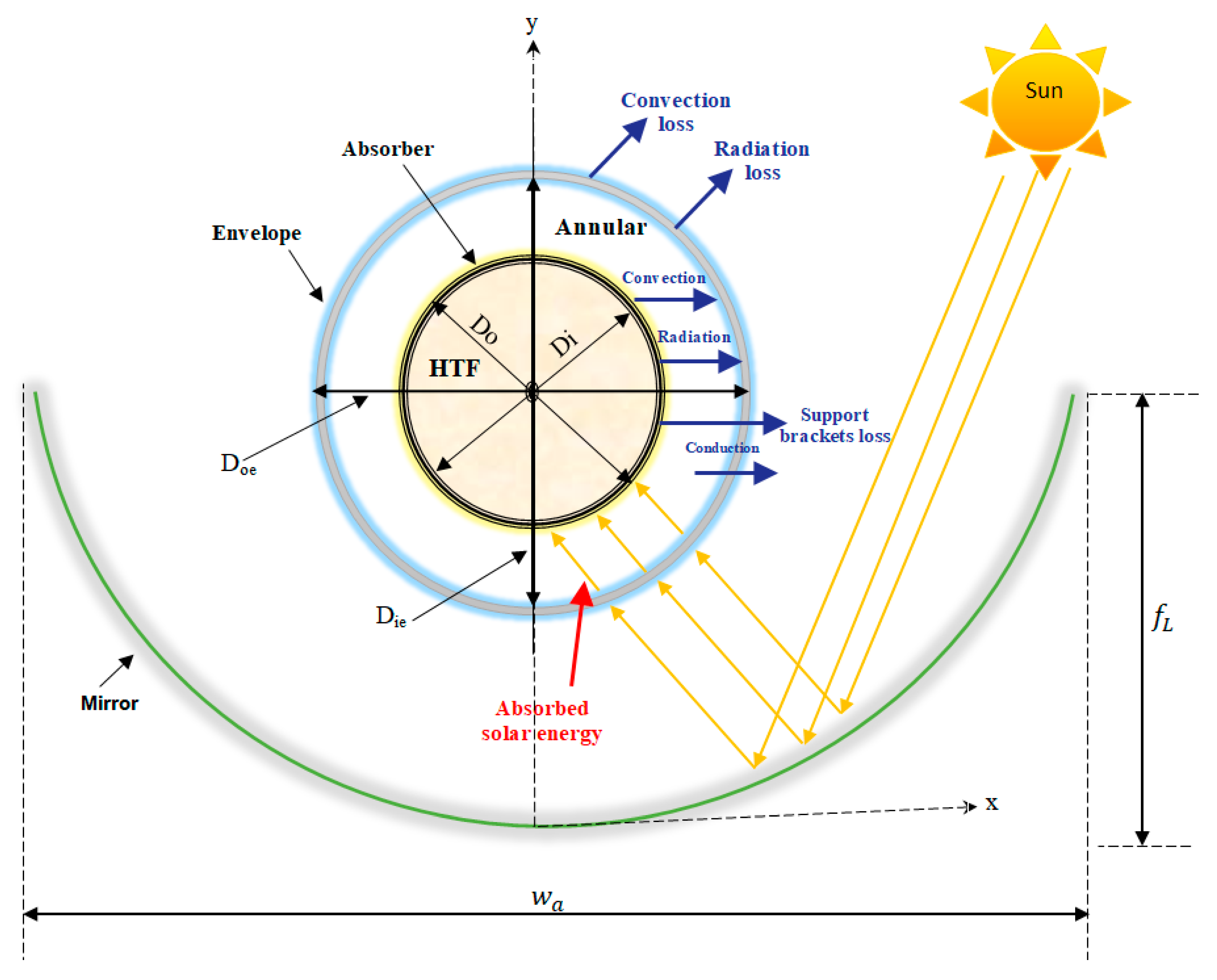
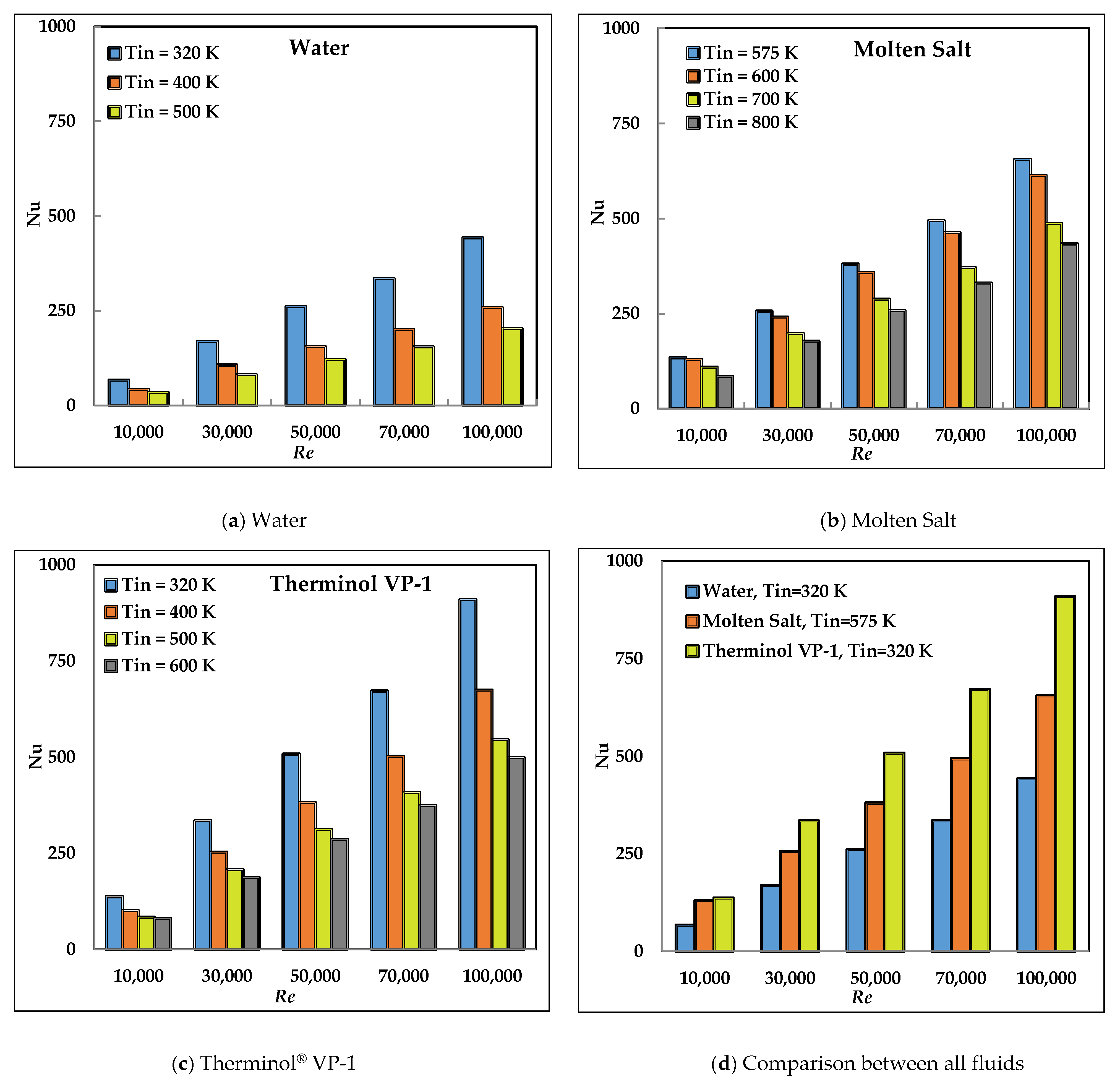
It is evident from the literature studies summarized above that changing the working fluid is a viable approach to optimize the thermal and hydraulic performance of the PTC systems. However, there are still some gaps in the literature especially when it comes to comparative studies among various heat transfer fluids in terms of thermal performance, hydraulic behavior and thermal stresses over a wide range of operating temperatures under realistic thermal environment. The present paper abridges this gap by presenting comparisons of various working fluids from different categories which are examined by means of numerical simulations taking into consideration the heat transfer performance, pumping power, thermal losses, thermal stresses and overall thermal efficiency under realistic non-uniform heat flux distribution using the Monte Carlo Ray Tracing (MCRT) model. Furthermore, the current study also outlines a parametric study where various fluid behaviors are analyzed under different operating conditions of inlet fluid temperature and Reynolds numbers. For example, water has been used with a temperature range of 320–500 K, Therminol^® VP-1 with a temperature range of 320–600 K, and molten salt with a temperature range of 575–800 K; in all these cases the range of Reynolds number values explored was Re = 10⁴–10⁵. The main objectives of this study are to examine the flow behavior through a parametric comparison of the heat transfer characteristics, and find the optimum operational conditions for different heat transfer fluids.

2. Mathematical Expressions of Parabolic Trough Collector Systems

A typical parabolic trough collector technology is schematically shown in Figure 1. In such systems, the solar energy is concentrated on long concave mirrors (which have a parabolic cross-section shape) called reflectors that reflect the solar energy to the solar absorber. The solar absorber is usually made of metal which is externally coated with selective absorber materials and located on the focal line of the reflectors. To minimize the thermal losses from the solar absorber, a glass sleeve is also often used. The received energy is transferred from the solar absorber to the working fluid (called also heat transfer fluid (HTF)) which is forced to flow through the absorber. The thermal energy mechanisms for the parabolic trough collector system depend on the thermal energy balance between the HTF and its surrounding. The solar energy from sun is focused onto the solar absorber and divided into two main parts. The first part crosses the absorber by conduction and is then transferred to the working fluid via convection. The second part is transferred to the glass sleeve by natural convection, radiation and conduction through the structural supports. The energy lost in the glass sleeve is transferred by radiation to the surroundings and by convection to the ambient.

2.1. Geometrical Design Formulations

The equation of the parabola shape used in a PTC system is U-shaped which can be expressed as:

$$y=\frac{x^2}{4f_L}$$

(1)

where x and y are the horizontal and vertical coordinates respectively with $f_L$ representing the location distance of the solar receiver which is calculated by Duffie et al. [28] as:

$$f_L=\frac{w_a}{4tan(\frac{{\phi }_r}{2})}$$

(2)

The parameter, $w_a$ represents the aperture width of the collector whereas ${\phi }_r$ is the rim angle which between the reflected beam radiation and the collector axis, defined by Duffie et al. [28] as:

$${\phi }_r=ta{n}^{-1}\left[\frac{8(\frac{f_L}{w_a})}{16{(\frac{f_L}{w_a})}^2-1}\right]=si{n}^{-1}(\frac{w_a}{2r_r})$$

(3)

In the above expression, the factor, $r_r$ represents the rim radius which is the maximum mirror radius and can be obtained from Duffie et al. [28] as:

$$r_r=\frac{2f_L}{1+cos{\phi }_r}$$

(4)

The aperture area, $A_a$ of the solar collector and the absorber area of the external surface, $A_o$ are read as:

$$A_a=w_{a}L$$

(5)

$$A_o=\pi D_{o}L$$

(6)

where, L represents the collector length. The ratio obtained by dividing the aperture area with the outer surface area called the geometrical concentration ratio (GCR) defined as:

$$GCR=\frac{A_a}{A_o}$$

(7)

2.2. Mathematical Expressions of Thermal Models

All parameters that are related to the thermal performance of the parabolic trough collector system are comprehensively clarified and explained in this section. These parameters are: the Nusselt number, Nu, the useful thermal energy, Q_u, the available solar energy, Q_s, thermal losses, Q_loss, the friction factor, f and the corresponding pressure drop, $\Delta P$. Based on the energy balance, the useful thermal energy collected by the working fluid can be expressed by Duffie et al. [28] as:

$$Q_u=\dot{m}{C}_p\left(T_{out}-T_{in}\right)$$

(8)

The variables ($T_{out}$ and $T_{in}$) are the outlet and inlet fluid temperatures respectively and $\dot{m}$ is the mass flow rate. Whereas the available solar energy, Q_s concentrated on the solar collector is given by Abed and Afgan [2] as:

$$Q_s=A_a{G}_b$$

(9)

Here the parameter, G_b is the direct normal irradiance. The thermal efficiency, ${\mathsf{\eta }}_{th}$ of the parabolic trough collector can thus be finally determined as:

$${\mathsf{\eta }}_{th}=\frac{Q_u}{Q_s}$$

(10)

To assess the overall thermal performance of the parabolic trough collector, the pumping power effect can be used to evaluate the overall thermal efficiency, ${\mathsf{\eta }}_o$ as suggested by Wirz et al. [29]:

$${\mathsf{\eta }}_o=\frac{Q_{u-}{W}_p/{\eta }_{el}}{Q_s}$$

(11)

Here the parameter, ${\eta }_{el}$ represents the power block electrical efficiency (taken as 32.7%) and the term, W_p is the pumping power in Watts which reads as:

$$W_p=\Delta P\dot{V}$$

(12)

In the above equation, the factor, $\dot{V}$ represents the volumetric flow rate whereas the term, $\Delta P$ represents the pressure drop which is determined from the Darcy–Weisbach equation given by Incropera et al. [30] as:

$$\Delta P=f\frac{L}{D_i}\frac{\rho U^2}{2}$$

(13)

$$f=\frac{8{\tau }_w}{\rho U^2}$$

(14)

The parameters $f$, L, $D_i$, $\rho$, U and ${\tau }_w$ are friction factor, the absorber length, the internal diameter of the solar absorber, the fluid density, flow velocity, and the wall shear stress respectively.

Based on the thermal energy balance, thermal losses from the glass sleeve transfers to the ambient by convection and to the sky by radiation, calculated by Bhowmik and Mullick [31] as:

$$Q_{loss}=L\pi D_{oe}{h}_{out}\left(T_{oe}-T_{am}\right)+L\pi D_{oe}\sigma {\epsilon }_{oe}(T_{oe}^4-T_{sky}^4)$$

(15)

Here the subscripts i, o, ie and oe refer to the internal surface of the solar absorber, external surface of the solar absorber, the internal surface of the glass envelope and the internal surface of the glass envelope respectively. Whereas the factor, $\sigma$ is the Stefan-Boltzmann coefficient which is 5.67 × 10⁻⁸ Wm⁻² K⁻⁴. However, in the absence of the glass sleeve from the parabolic trough collector system (as in the current study), the thermal losses transfer directly from the absorber receiver as expressed by Bhowmik and Mullick [31] are:

$$Q_{loss}=L\pi D_o{h}_{out}\left(T_o-T_{am}\right)+L\pi D_o\sigma {\epsilon }_o(T_o^4-T_{sky}^4)$$

(16)

where the parameter, $h_{out}$ represents the ambient heat transfer coefficient which is suggested by Bhowmik and Mullick [31] as:

$$h_{out}=4V_w^{0.58}{D}_o^{-0.42}$$

(17)

Here the factor, V_w represents the wind speed of the flow outside the solar receiver, taken as 0.5 m/s in the current study. Whereas the parameter, ${\epsilon }_o$ represents the emissivity of the external surface of the solar absorber which is a function of the external surface temperature of the solar absorber, selective coatings and absorber materials. In the current study, the investigated model is very similar to the model examined experimentally by Dudley et al. [32], which can be expressed as:

$${\epsilon }_o=0.062+2\times {10}^{-7}\times T_O^2$$

(18)

The sky temperature, $T_{sky}$ which depends strongly on the ambient temperature can be calculated by the expression given by Swinbank [33] as:

$$T_{sky}=0.0552T_{am}^{1.5}$$

(19)

On the other hand, the useful thermal power, $Q_u$ carried by the working fluid can be calculated using the Newton’s cooling law taking the fluid convection heat transfer coefficient as defined by Duffie et al. [28] as:

$$Q_u=h{A}_i\left(T_i-T_f\right)$$

(20)

Here the term, A_i represents the internal surface area of the absorber tube. However, depending on the convection heat transfer coefficient, h, the absorber diameter, $D_i$ and the fluid thermal conductivity, k, the Nusselt number, Nu can be calculated as:

$$Nu=\frac{h{D}_i}{k}$$

(21)

Apart from the $Nu$ number, two other non-dimensional parameters are also important which are the Reynolds, $Re$ number and the Prandtl, $Pr$ number. These parameters are defined as:

$$Re=\frac{\rho U{D}_i}{\mu }$$

(22)

$$Pr=\frac{\mu C_p}{k}$$

(23)

The parameters, C_p and µ are the fluid specific heat capacity and the fluid dynamic viscosity respectively. The flow is assumed to be turbulent in the solar absorber applications if the $Re$ number is larger than or equal to 4000. The $Nu$ number of the solar absorber in the turbulent flow regime can be predicted using empirical correlations available in the literature such as those of Petukhov [34] or Gnielinski [35] which are expressed as:

$$Nu=\frac{\left(\frac{f}{8}\right)RePr}{1.07+12.7{\left(\frac{f}{8}\right)}^{0.5}(P{r}^{\frac{2}{3}}-1)}for\left\{\begin{array}{c}0.5\le Pr\le 2000\\ {10}^4<Re<5\times {10}^6\end{array}\right\}$$

(24)

$$Nu=\frac{\left(\frac{f}{8}\right)\left(Re-1000\right)Pr}{1+12.7{\left(\frac{f}{8}\right)}^{0.5}(P{r}^{\frac{2}{3}}-1)}for\left\{\begin{array}{c}0.5\le Pr\le 2000\\ 3\times {10}^3<Re<5\times {10}^6\end{array}\right\}$$

(25)

The factor, f represents the friction factor inside the solar receiver is generally a function of only the $Re$ number in a typical solar receiver and can thus be expressed by the empirical correlations of Petukhov [34] as:

$$f={\left(0.75LnR{e}^{-1.64}\right)}^{-2}for\left\{3000<Re<5\times {10}^6\right\}$$

(26)

These empirical correlations of $Nu$ number and friction factor are used in the current study to validate the numerical predications.

3. Fluid and Material Properties

3.1. Parabolic Trough Collector Design

The optical and geometrical characteristics used in the current study in addition to environmental parameters are listed in

Table 1. The PTC model parameters used in the current work.

Property	Value	Property	Value
Absorber internal diameter, Di (m)	0.066	Solar beam irradiation, Gb (W/m2)	1000
Absorber external diameter, Do (m)	0.07	Concentration ratio, C	37
Aperture width, wa (m)	8.0	Wind speed, V (m/s)	0.5
Solar receiver length, L (m)	4.0	Ambient temperature, Tam (K)	300
Focal length, fL (m)	1.84	Rim angle, ${\phi }_r$ (Deg.)	95

. For simplicity, the glass envelope is entirely removed in the current study, duplicating approximately the same model as (LS-2) developed by Dudley et al. [32], for the bare case.

3.2. Thermal Properties of Working Fluids

In order to achieve precise results, it is necessary that the thermal properties of HTF are accurately incorporated in the simulations. In the present work, three different working fluids are used as base fluids; water, Therminol^® VP-1 and molten salt (60% sodium nitrate (NaNO₃), 40% potassium nitrate (KNO₃)). The thermal properties of water are listed in

Table 2. Thermal properties of water at different inlet temperatures, Incropera [30]. Density, $\rho$, dynamic viscosity, μ, specific heat capacity, C_p and thermal conductivity, k.

Tin (K)	μ (kg/m·s)	$\mathit{\rho }$ (kg/m³s)	Cp (J/kg·k)	k (w/m·k)	Pr
320	0.000577	989.12	4180	0.64	3.77
400	0.000217	937.207	4256	0.688	1.34
500	0.000118	831.2552	4660	0.642	0.86

.

For the Therminol^® VP-1 base fluid, the temperature-dependent thermal properties which are valid for a temperature range of (285.15 K ≤ T ≤ 698.15 K) are given by Mwesigye et al. [36] as:

$$\rho =1.4386\times {10}^3-1.8711T+2.737\times {10}^{-3}{T}^2-2.3793\times {10}^{-6}{T}^3\left(\mathrm{kg}·{\mathrm{m}}^{-3}\right)$$

(27)

$$C_p=2125-11.017T+0.049862T^2-7.7663\times {10}^{-5}{T}^3+4.394\times {10}^{-8}{T}^4\left({\mathrm{Jkg}}^{-1}{\mathrm{K}}^{-1}\right)$$

(28)

$$k=0.14644+2.0353\times {10}^{-5}T-1.9367\times {10}^{-7}{T}^2+1.0614\times {10}^{-11}{T}^3\left({\mathrm{Wm}}^{-1}{\mathrm{K}}^{-1}\right)$$

(29)

$$\begin{array}{c}\mu =3.661\times {10}^2-3.0154T+8.3409\times {10}^{-3}{T}^2-7.723\times {10}^{-6}{T}^3\left(\mathrm{mPa}·\mathrm{s}\right)\\ \mathrm{For}285.15\mathrm{K}\le T\le 373.15\mathrm{K}\end{array}$$

(30)

$$\begin{array}{c}\mu =23.165-0.1476T+3.617\times {10}^{-4}{T}^2-3.9844\times {10}^{-7}{T}^3+1.6543\times {10}^{-10}{T}^4\\ \left(\mathrm{mPa}·\mathrm{s}\right)\mathrm{For}373.15\mathrm{K}\le T\le 698.15\mathrm{K}\end{array}$$

(31)

However, for the molten salt the temperature dependent thermal properties which are valid for a temperature range of (573.15 K ≤ T ≤ 873.15 K) are given by Pacheco et al. [37] as:

$$\rho =2090-0.636T\hspace{1em}\hspace{1em}\hspace{1em}\left(\mathrm{kg}·{\mathrm{m}}^{-3}\right)$$

(32)

$$C_p=1443+0.172T\hspace{1em}\hspace{1em}\hspace{1em}\left({\mathrm{Jkg}}^{-1}{\mathrm{K}}^{-1}\right)$$

(33)

$$k=0.443+1.9\times {10}^{-4}T\hspace{1em}\hspace{1em}\hspace{1em}\left({\mathrm{Wm}}^{-1}{\mathrm{K}}^{-1}\right)$$

(34)

$$\mu =22.714-0.12T+2.281\times {10}^{-4}{T}^2-1.474\times {10}^{-7}{T}^3\left(\mathrm{mPa}·\mathrm{s}\right)$$

(35)

Note that the temperature in molten salt equations is in (°C).

3.3. Material Properties of Solid Part

As recommended by Forristall [14], 321H stainless steel is used in the present study for the solid pipe due to its low bending behavior and high strength capability. Properties of 321H stainless steel are given in

Table 3. Mechanical and thermal properties of absorber material.

Property	Value	Property	Value
Thermal conductivity, ksolid (W/m K)	17.3	Modulus of elasticity, E (GPa)	193
Specific heat capacity, Csolid (J/kg K)	512	Poisson’s ratio, $\upsilon$	0.28
Thermal expansion coefficient, $\beta$ (1/°C)	1.89 × 10−5	Material Density, $\rho$ solid (kg/m3)	8050

.

3.4. Turbulence Models Implemented in the Present Work

3.4.1. Launder and Sharma k-ε Model

This model was developed by Launder and Sharma [38] to predict the flow phenomena in flow applications like duct flows and heat transfer applications. This is a low Re treatment model which requires Y⁺ of one near solid walls. This is a two-equation model which solves one transport equation for the turbulent kinetic energy, $k$ and another equation for the quasi-homogeneous dissipation rate, $\check{\epsilon }$. The model equations are shown in

Table 4. Description of the Launder and Sharma k-ε model, Equations taken from Launder and Sharma [38].

Term Description	Comment
${\mathcal{V}}_t=c_{\mu }{f}_{\mu }\frac{k^2}{\check{\epsilon }}$	The kinematic eddy viscosity.
$\frac{Dk}{Dt}=P_k-\left(\check{\epsilon }+2\mathcal{V}{\left(\frac{\partial k^{0.5}}{\partial x_j}\right)}^2\right)+\frac{\partial }{\partial x_j}\left(\left(\mathcal{V}+{\mathcal{V}}_t\right)\frac{\partial k}{\partial x_j}\right)$	Turbulent kinetic energy equation.
$\frac{D\check{\epsilon }}{Dt}=c_{\epsilon 1}\check{\epsilon }\frac{P_k}{k}-c_{\epsilon 2}{f}_2\frac{{\check{\epsilon }}^2}{k}+E+\frac{\partial }{\partial x_j}\left(\left(\mathcal{V}+\frac{{\mathcal{V}}_t}{{\sigma }_{\epsilon }}\right)\frac{\partial \check{\epsilon }}{\partial x_j}\right)$	The quasi-homogeneous dissipation rate equation
$\check{\epsilon }=\epsilon -2\mathcal{V}{\left(\frac{\partial k^{1/2}}{\partial x_j}\right)}^2$	Definition of the quasi-homogeneous dissipation rate.
$f_2=1-0.3\exp \left(-R_t{}^2\right)and{R}_t=k^2/\mathcal{V}\epsilon$	$f_2$: Damping function and $R_t$: Turbulent Reynolds number.
$E=2\mathcal{V}\ast {\mathcal{V}}_t\ast {\left(\frac{{\partial }^2{U}_i}{\partial x_j\partial x_k}\right)}^2$	Extra source term.
$f_{\mu }=exp\left(\frac{-3.4}{{\left(1+\frac{R_t}{50}\right)}^2}\right)$	Damping function
$c_{\epsilon 1}=1.44,c_{\epsilon 2}=1.92$	Model constants

.

3.4.2. The k-ω Shear Stress Transport Model

This eddy-viscosity model proposed by Menter [39] also solves two separate transport equations, one for the turbulent kinetic energy, $k$ and the other for the specific dissipation rate, ω. This model can be used down to the wall (low-Re treatment model) without considering any extra damping functions. The model switches between k-ω and k-ε approaches depending upon the distance to the solid wall. The model as illustrated in

Table 5. Description of the SST k-ω model, Equations taken from Menter [39].

Term Description	Comment
${\mathcal{V}}_t=\frac{a_{1}k}{\max \left(a_1\omega ,\mathsf{\Omega }{F}_2\right)}$	The kinematic eddy viscosity.
$\frac{Dk}{Dt}=\left(\frac{{\tau }_{ij}}{\rho }\right)\frac{\partial U_i}{\partial x_j}-{\beta }^{*}k\omega +\frac{\partial }{\partial x_j}\left[\left(\upsilon +{\sigma }_k{\nu }_t\right)\frac{\partial k}{\partial x_j}\right]$	Turbulent kinetic energy equation.
$\frac{D\omega }{Dt}=\frac{\gamma }{{\nu }_t}\left(\frac{{\tau }_{ij}}{\rho }\right)\frac{\partial U_i}{\partial x_j}-\beta {\omega }^2+\frac{\partial }{\partial x_j}\left[\left(\upsilon +{\sigma }_{\omega }{\nu }_t\right)\frac{\partial \omega }{\partial x_j}\right]+2\left(1-F_1\right){\sigma }_{\omega 2}\frac{1}{\omega }\frac{\partial k}{\partial x_j}\frac{\partial \omega }{\partial x_j}$	Specific dissipation rate equation
$F_1=\tanh \left(arg{.}_1^4\right),arg{.}_1=\min \left(\max \left(\frac{\sqrt{k}}{0.09\omega y},\frac{500\nu }{y^2\omega }\right),\frac{4\rho k{\sigma }_{\omega 2}}{C{D}_{kw}{y}^2}\right),$ $C{D}_{kw}=\max \left(2\rho {\sigma }_{\omega 2}\frac{1}{\omega }\frac{\partial k}{\partial x_j}\frac{\partial \omega }{\partial x_j},{10}^{-20}\right)$	F1: The first blending function. CD: cross diffusion.
$F_2=\tanh \left(arg{.}_2^2\right),arg{.}_2=\max \left(\frac{2\sqrt{k}}{0.09\omega y},\frac{500\nu }{y^2\omega }\right)$	F2: The second blending function.
$\varphi ={\varphi }_1{F}_1+{\varphi }_2\left(1-F_1\right)$	The interpolating function.
${\gamma }_1=\raisebox{1ex}{${\beta }_1$}\!\left/ \!\raisebox{-1ex}{${\beta }^{*}$}\right.-\raisebox{1ex}{${\sigma }_{\omega 1}{k}^2$}\!\left/ \!\raisebox{-1ex}{$\sqrt{{\beta }^{*}}$}\right.$	Constants of group1 (φ1) (the k-ω model).
${\gamma }_2=\raisebox{1ex}{${\beta }_2$}\!\left/ \!\raisebox{-1ex}{${\beta }^{*}$}\right.-\raisebox{1ex}{${\sigma }_{\omega 2}{k}^2$}\!\left/ \!\raisebox{-1ex}{$\sqrt{{\beta }^{*}}$}\right.$	Constants of group2 (φ2) (the standard k-ε model).
${\mathrm{a}}_1=0.31,$${\mathsf{\sigma }}_{\mathsf{\omega }1}=0.5,{\mathsf{\sigma }}_{\mathsf{\omega }2}=0.856,\mathrm{k}=0.41,{\mathsf{\beta }}^{*}$=0.09, ${\mathsf{\beta }}^1=0.075,{\mathsf{\beta }}^2=0.0828,{\mathsf{\sigma }}_{\mathrm{k}1}=0.85,{\mathsf{\sigma }}_{\mathrm{k}2}$=1.	Model constants

.

4. Numerical Model Validation

4.1. Mesh Independence Study

For the considered range of $Re$ number, the non-dimensional variable, Y⁺ is less than 1. To obtain this, the distance between the first cell and the wall was adjusted as the $Re$ number varied. By increasing the $Re$ number, the distance from the solid wall has to be decreased as the boundary layer thickness becomes thinner due to an increase in the turbulence level. For the present work the geometry consisted of a 66 mm inner tube diameter, 70 mm outer tube diameter and 4 m tube length. Three different grids were used in order to study the effect of the resolution on the solution; namely Coarse mesh with 0.8 million cells, medium mesh with 1.8 million cells and fine mesh with 2.4 million cells, shown in Figure 2. All grids were very fine in the near-wall region in order to resolve the viscous sub-layer as the Y⁺ ≈ 1 is considered in the near-wall node.

The predicted $Nu$ numbers versus $Re$ numbers for all three grids were compared using pure water at inlet temperature of 320 K over a range of $Re$ number (10⁴–10⁵) as shown in Figure 3. As can be seen, the coarse grid failed to predict the $Nu$ number in regimes of the high level of turbulence. After increasing the mesh size in all directions, the new medium mesh was able to capture the thermal physics precisely even in high turbulent-level regions. However, by increasing the mesh size further to Fine level did not change the results. Therefore, the medium grid was found to be the sufficient grid for the present study. The mesh properties of the medium size are (cell type: hexahedra, mesh average non-orthogonally: 8.1, maximum skewness is 0.7 and has no negative volume cell).

4.2. OpenFOAM Software

In the current work, open-source CFD software Open Field Operation and Manipulation (OpenFOAM) was used. This C++ based open source software was selected as its gives the user the option to modify any part of the code such as thermo-physical properties, numerical schemes, boundary conditions, discretization methods etc.. Within the OpenFOAM library, a solver named conjugated heat transfer multi region simple foam (chtMultiRegionSimpleFoam) was utilized in the present study. This solver can be used for simulating the flow characteristics and heat transfer in conjugate solid-fluid problem cases with no limitations for solid or fluid regions. A second order accurate central differencing scheme was used for all spatial discretizations. For turbulent quantities, the van Leer scheme [40] was used for all the RANS equations with the exception of the momentum equation in which the second-order accurate upwind scheme was employed. Finally, the pressure velocity coupling was handled using the PISO algorithm Issa [41]. The boundary conditions used in the present study are described in

Table 6. Boundary condition of fluid and solid variables applied in the current study; FV: means fixed value and ZG: means zero gradients.

Boundary	U (m/s)	P (Pa)	T (K)	K (m2/s2)	ε (m2/s3)	ω (1/s)
Inlet-fluid	FV	ZG	Value	FV	FV	FV
Outlet-fluid	ZG	Zero	ZG	ZG	ZG	ZG
Fluid-solid	ZG	fixedFluxPressure	FV	Zero	Zero	∞
Inner wall	No-slip	Calculated	FV	Zero	Zero	Zero
Outer wall	No-slip	Calculated	See Appendix A	Zero	Zero	Zero
Inlet-solid	No-slip	Calculated	ZG	Zero	Zero	Zero
Outlet-solid	No-slip	Calculated	ZG	Zero	Zero	Zero

.

4.3. Numerical Model Validation

To obtain an accurate prediction of the solar absorber behavior using the two aforementioned turbulence models, several steps were taken for validation. Firstly, the output temperature of working fluid was validated by using the same geometry and thermal environment conditions as that of Dudley et al. [32] which preformed experiments of a parabolic trough collector without glass envelope using Syltherm 800 oil as HTF at Sandia national laboratories.

Table 7. A comparison between the experimental data and numerical predictions of the output temperature of working fluid.

Dudley et al. [32]				k Omega SST		LS k Epsilon
$\dot{\mathit{V}}$ (L/min)	Gb (W/m2)	Tin (°C)	Tout (°C))	Tout (°C))	Dev. (%)	Tout (°C))	Dev. (%)
48.4	801.3	151.7	166.2	168.337	−1.286	171.347	−3.097
49.8	888.6	198.2	215.5	213.294	1.024	215.425	0.035
51.1	920.5	301	314.2	313.809	0.124	314.833	−0.201
55.6	929.4	313.8	324.8	325.340	−0.166	326.375	−0.485
55.8	940.4	384	395	395.446	−0.113	396.435	−0.363
50.9	935.7	252.1	268	266.868	0.422	267.360	0.239
39.8	817.5	101	120.8	127.859	−5.844	136.211	−12.757
50.1	854.5	203.1	219.2	217.292	0.870	219.364	−0.075
50	867.6	203.4	219.6	217.825	0.808	219.210	0.178
48.2	922	100.8	121.1	125.409	−3.558	131.945	−8.955
51.6	927.6	354.4	367.8	366.507	0.352	367.572	0.062
Average Deviations (%):				−0.670		−2.311

presents the experimental test conditions compared with the numerical results of both turbulence models. It should be noted here that for every single volumetric flow rate, $\dot{V}$ the other test conditions such as wind speed, inlet temperature, T_in, ambient temperature, T_am and direct normal irradiance, G_b, were varied.

It can be observed from Table 7 that the k-ω SST model performed better as it predicted output temperatures, T_out closer to the experimental data with an average deviation of only 0.67%. The second parameter selected for the validation was the thermal efficiency of the parabolic trough collector with realistic heat flux boundary condition (non-uniform) on the external wall of the solar absorber. The numerical results produced by the considered turbulence models were validated with experimental measurements of the Dudley et al. [32] as presented in Figure 4.

It can be seen from the Figure 4 that the k-ω SST turbulence model predicted the thermal efficiency better than the LS k-epsilon model especially for the lower inlet temperature cases. The model was also validated for the $Nu$ number of pure water moving inside the solar receiver with the experimental correlations of Petukhov [34] and Gnielinski [35] as shown in Figure 5a. Here it can again be observed that the LS k-epsilon model under predicted the $Nu$ number compared to the k-ω SST model and the correlations. The last experimental correlation of Petukhov [34] for the friction factor was also used to validate the numerical results of the k-ω SST turbulence model only as shown in Figure 5b. This correlation is for a fully developed turbulent flow. As shown in the figure that the agreement between numerical results and experimental data is very good in all turbulent regimes. Form all the validation figures presented above, it can be deduced that the k-ω SST model is the better choice and was hence used for all the remaining simulations.

5. Results and Discussion

5.1. Heat Transfer Performance

Figure 6a–c present the $Nu$ number as a function of the $Re$ number at different inlet temperatures for the three working fluids; water, molten salt and therminol VP-1. It can be seen that the trend is similar for the $Nu$ numbers at the inlet temperatures of all working fluids. The $Nu$ number increases considerably as the $Re$ number increases for all working fluids.

This can be attributed to several reasons; lower inner wall temperature of the solar absorber, thinner thickness of the boundary layer at larger $Re$ number and lower output temperature of the working fluid. Furthermore, by increasing the inlet temperature, the thermal properties of working fluids change consequently, leading to a decrease in the $Pr$ number which results in a lower $Nu$ number prediction. Another important feature that can be noted from this figure is that the working fluid at the smallest inlet temperature provided the largest $Nu$ number for all HTF’s due to the larger provided $Pr$ number. The previous studies such as Mwesigye et al. [36] have also reported similar behavior. Figure 6d shows the Nu profile of all the fluids at the smallest inlet temperature as a function of $Re$ number. It is noticeable that the $Nu$ number of Therminol^® VP-1 is the largest for all $Re$ numbers followed by molten salt and water. This is due to the thermal properties of therminol VP-1 which leads to a larger $Pr$ number at all inlet temperatures compared to the other fluids; the $Pr$ number of Therminol^® VP-1 is 2.5 times larger than that of molten salt and 6 times greater than that of water. According to the results obtained at the smallest fluid temperature and largest $Re$ number, the $Nu$ number predicted using Therminol^® VP-1 is greater than that predicted by water and molten salt by 2.055 and 1.4 times, respectively.

5.2. Collector Hydraulic Performance

Figure 7a–c present the specific pressure drop behavior (Pa/m) of all base fluids at different inlet temperatures. It can be noticed that the specific pressure drop increases significantly as the $Re$ number increases. This is expected since the mass flow rate increases gradually as $Re$ number increases and the flow becomes highly turbulent; thus, higher pumping power is required to force the flow through the solar absorber. Moreover, the specific pressure drop of all fluids decreases as the temperature of the working fluid increases due to the temperature dependent properties. Similar findings were reported by the previous studies of Arslan et al. [27] and Mwesigye et al. [36].

Figure 7d presents the specific pressure drop distribution of all fluids at the smallest inlet temperature as a function of the $Re$ number. It is very clear that the specific pressure drop of molten salt is the largest for all $Re$ numbers followed by Therminol^® VP-1 and then water. This is because the molten salt fluid flow characteristics (density and viscosity) are relatively higher compared to the other fluids; density approximately 1.8 and 2 times higher and viscosity approximately 2 and 5.7 times higher than that of Therminol^® VP-1 and water, respectively. Overall, at the minimum fluid temperature and maximum $Re$ number, the specific pressure drop predicted by molten salt is larger than that predicted by water and therminol VP-1 by 16.5 and 1.2 times, respectively.

5.3. Thermal Losses

For the thermal loss analysis of the solar receiver, the main objective is to determine the major factor that affects these thermal losses when the glass envelope is removed. It is observed that the average temperature of the receiver’s outer surface is strongly dependent on the inlet fluid temperature. The smaller the inlet fluid temperature the lower the outer surface absorber’s temperature, consequently leading to a decrease in thermal losses thereby improving the thermal gain. Among the thermal losses of the solar receiver, the radiation loss is a function of forth-power absolute temperature difference between the outer surface temperature and sky temperature. Since the glass envelope is removed in this study, the outer surface of the solar receiver is greatly radiated. Therefore, the radiation thermal loss is quite sensitive to the absorber’s surface temperature rather than the ambient condition. Thus, radiation loss from absorber surface to the sky increase gradually. The second important contribution to thermal losses is the convection heat loss from the outer surface to the ambient air which is approximately from 60 to 70% as shown in Figure 8. This is in complete agreement with the findings of Dudley et al. [32]. These types of losses are a function of two important factors; the outside air heat transfer coefficient and the temperature difference between the receiver outer surface and ambient air.

Figure 9 exhibits the results of thermal losses as a function of operating temperature for all the respective fluids at different mass flow rates. As already mentioned, the outer surface temperature increases considerably with increasing operating temperatures, this significantly enhances the convective heat loss. This behavior is in perfect agreement with Forristall [14], Bellos et al. [22] and Dudley et al. [32]. It is observed that the smaller $Re$ numbers are associated with the largest thermal losses for all the cases under consideration. This is because the flow with smaller velocity acts to absorb more energy and reflects part of it to the inner surface via convection and from the inner surface to the outer surface via conduction leading to an enhancement of the outer surface’s temperature. On the other hand, the solar absorption starts to reduce once the flow velocity increases, leading to energy reduction in the reflected parts. The figure shows that the largest heat losses are obtained when using molten salt due the higher operating temperatures. However, for the fluids with same inlet temperatures (i.e. water and Therminol^® VP-1) at 500K, the thermal losses produced by Therminol^® VP-1 are larger than those produced by water by 1.2 times. Another important characteristic that can be highlighted here is that the convection heat losses can be highly affected by the wind velocity, especially in the case of no glass envelop. For the no glass envelop case, the ambient air derived by the forced convention is very large and can be decreased by reducing the ambient wind as presented in Figure 9d. However, in the case of zero air velocity, the convection heat losses should be naturally determined rather than forced convection.

5.4. Overall Collector Efficiency

The thermal efficiency of the bare receiver (without glass sleeve) is presented in Figure 10 for all fluids over a range of inlet operating temperatutres of (320–800) K and different $Re$ numbers. It can be observed that all the working fluids show similar thermal behaviour in terms of the thermal efficiency which is directly proportional to the inlet operating temperature. In general, the smaller the inlet working temperature, the larger the receiver thermal efficiency. The reason behind is that by increasing the fluid inlet temperature, the outer surface of the solar receiver becomes highly radiated leading to a significant increase in radiation and convection losses. In other words, larger absorber temperature at the outer surface acts to increase thermal losses and consequently reduces the overall thermal efficiency with lower pumping power requirements. However, by increasing the $Re$ number for all cases at a given inlet operating temperature, moderate reduction can be observed in the overall thermal efficiency. This is because to achieve higher $Re$ numbers the flow rate needs to increase which obviously requires larger pumper power, leading to a reduction in the heat gain as can be noted from the efficiency equation. This means that for the same fluid, the thermal efficiency can either be affected by thermal losses (which are dependent upon the inlet fluid temperature) or by the pumping power requirement (which is dependent upon the desired flow rate). This behavior is in agreement with the findings of Forristall [14], Bellos et al. [23], Islam et al. [24] and Dudley et al. [32].

It is prudent to note here that the Therminol^® VP-1 preforms more or less the same as molten salt for the common temperature range whereas the Therminol^® VP-1 is the most ideal fluid for the temperature range of 320–500 K. Furthermore, the thermal properties of fluids play an important role in terms of the absorbed heat gain. For example, the mass flow rates (m^◦) of water and therminol VP-1 are not the same even at the same $Re$ number and inlet fluid temperature as illustrated in

Table 8. A comparison between the thermal performances of water and Therminol^® VP-1.

	Water		Therminol® VP-1		Water		Therminol® VP-1
Re	m (kg/s)	Qu (W)	m (kg/s)	Qu (W)	m (kg/s)	Qu (W)	m (kg/s)	Qu (W)
	Tin = 320 K				Tin = 400 K
10,000	0.29	15,463.05	1.14	22,126.8	0.112	12,850.22	0.38	17,657.12
30,000	0.89	12,451.31	3.44	19,534.16	0.33	12,250.78	1.13	15,558.12
50,000	1.49	12,268.03	5.73	18,038.55	0.56	11,221.59	1.9	14,926.81
70,000	2.09	12,335.38	8.02	17,014	0.787	11,306.02	2.65	14,473.58
100,000	2.9	13,292.31	11.46	15,902.94	1.12	11,511.28	3.8	13,961.22

. It is clear that the mass flow rates of therminol VP-1 are larger than those of water by approximately four times at all $Re$ numbers and both inlet temperatures. This enhances the thermal energy gain (Q_u) for Therminol^® VP-1 significantly compared to that of water. It is interesting to note here that at higher inlet temperatures (more than 400 °C) the Therminol^® VP-1 no longer works well which in turn leads to a poor Rankine cycle yield, in other words reducing the thermal efficiency of the power plant. It is thus concluded that molten salt is a better candidate at these higher temperatures.

5.5. Thermal Stresses

Another important parameter considered in this work are the thermal stresses in the solid part in the circumferential direction of the absorber tube. The circumferential stress, ${\sigma }_{\theta }$ given by Barron and Barron [42] reads as:

$${\sigma }_{\theta }=-\frac{\beta E\Delta T}{2\left(1-v\right)}\left[\frac{1+\ln \left(r/r_o\right)}{\ln \left(r_i/r_o\right)}+\frac{{\left(r_o/r\right)}^2+1}{{\left(r_o/r_i\right)}^2-1}\right]$$

(36)

where, $\beta$ is the thermal expansion of the solid material (1/°C), $E$ is the modulus of elasticity (Pa), $\Delta T$ is the temperature difference between the outer and inner surfaces (°C), and $v$ is the Poisson’s ratio. Where at $r=r_i$, the circumferential stress in the above equation represents the tensile force at the inner surface and at $r=r_o$, the stress represents compression at the outer surface. Where $r_i$ and $r_o$ are the receiver inner and outer radiuses respectively.

Structural thermal stresses are a result of the temperature differential between the two sides of the material in the presence of restrictions. These types of stresses, in fact, are mechanical stresses happening due to forces caused by a metal part that tries to contract or expand when it is restricted. Theoretically speaking if there were no restrictions, there would not be any thermal stresses. For the case of parabolic trough collectors, the solar receivers both ends are rigidly fixed and are subjected to a thermal difference between the inner and outer surfaces. Thereby, generating thermal stresses; compressive at the outer surface and tensile stresses at the inner surface. Here two types of restrictions can be addressed; external and internal restrictions. The external restriction caused by the support brackets at the receiver ends which prevents contraction or expansion in the whole system in the presence of temperature difference.

Thermal stresses in the circumferential direction due to the temperature gradient in the solar absorber material are shown in Figure 11 for all fluids considered in this study. The positive upper curves represent the tensile stresses whereas the negative lower curves represent the compressive stresses. It is noticed that the circumferential stresses are approximately symmetrical for all flow conditions and all working fluids. For different inlet temperatures both the compressive and tensile stresses increase till a certain $Re$ number and then become constant for all the fluids. This is because an increase in the $Re$ number leads to a decrease in the boundary layer thickness and thus the temperature of the outer surface becomes closer to that of the inner surface. Another important feature that can be noticed from this figure is that the inlet fluid temperature plays a very important role in determining the circumferential stresses; especially, in the low-level turbulence regimes (i.e. low $Re$ numbers). At low $Re$ numbers an increase in the inlet fluid temperature leads to a reduction of the flow $Pr$ number, this in turn leads to an increase in the thickness of the thermal boundary layer. The larger the inlet fluid temperature, the smaller the $Pr$ number leading to smaller tensile circumferential stresses and larger compressive circumferential stresses. The thermal stresses presented by Therminol^® VP-1 are smaller than those depicted by other fluids particularly in the low-turbulence regimes for all inlet fluid temperatures. On the other hand, no significant changes were observed when the inlet fluid temperature was increased, particularly from 575 to 700 K.

5.6. Velocity and Temperature Contours

Figure 12 depicts the velocity contours of the outlet wall of the solar receiver for all fluids at the smallest inlet temperatures (320 K for water and therminol VP-1 and 575 K for molten salt). The cases presented are for the smallest $Re$ number i.e. 10,000. It is observed from this figure that there is no difference in the flow patterns in terms of velocity contours since all fluids generally behave similar due to the no slip wall boundary condition. However, the magnitude of velocity profiles is different due to a difference in the thermal behavior for each fluid as discussed previously.

The non-uniform heat flux distribution on the external wall of the solar receiver is very obvious in the temperature contours of all the fluids as presented in Figure 13. It is very clear that the type of fluid could affect the temperature distribution even if they enter the PTC with the same inlet temperature and are subjected to the same heat flux boundary condition by the external walls. For instance, the temperature contour map of water is between 320 K (minimum) and 390 K (maximum) while the temperature contour distribution of Therminol^® VP-1 is between 320 K (minimum) and 470 K (maximum). Furthermore, it is evident that the lower solid half of the solar absorber is exposed to larger-temperature variation compared to the upper half due to the non-uniform heat flux around the external wall of the solar receiver. For the fluid part, it is clear that the fluid temperature is very high close to the wall and reduces gradually away from the solid wall reaching minimum values at the top part of the receiver as depicted by the two recirculation regions generated for the water and therminol VP-1 cases.

5.7. Mean Temperature Profiles

The non-dimensional mean temperature, T⁺ of all considered working fluids normalized by the friction temperature, T_τ is another parameter that can be used to study the effect of change in the working fluid on the thermal performance. This parameter can be calculated as:

$$T^{+}=\frac{\langle T_w\rangle -T}{T_{\tau }}$$

(37)

where, $\langle T_w\rangle$ represents the average internal wall temperature, $T$ is the fluid temperature distribution from the wall to the absorber centre and $T_{\tau }$ represents the friction temperature which can be expressed as

$$T_{\tau }=\frac{q_w}{\rho C_p{U}_{\tau }}$$

(38)

Here the variables $q_w,\rho$ and $C_p$ are the heat flux, the fluid density and the fluid specific heat capacity, respectively. In Equation (37), the parameter, $U_{\tau }$ represents the friction velocity which is a function of the wall shear stress and fluid density calculated as follows:

$$U_{\tau }=\sqrt{{\tau }_w/\rho }$$

(39)

For the simulations, $Y^{+}$ is a function of the first cell height, y, friction velocity and kinematic fluid viscosity, $\nu$ and can be calculated from the following expression:

$$Y^{+}=\frac{y{U}_{\tau }}{\nu }$$

(40)

Figure 14 shows the mean temperature profiles close to the absorber outlet (at L = 3.8 m) under uniform heat flux for all considered working fluids at specific $Re$ numbers (in this case Re = 10,000). It is observed from these profiles that an increase in the fluid inlet temperature leads to a gradual decrease in the mean temperature profiles inside the logarithmic region, away from the walls. This is accompanied by a gradual decrease in the heat conduction sub-layer close to the wall (at smaller Y⁺ values). This is because an increase in the inlet fluid temperature leads to a gradual decrease of the effective $Pr$ number. On the other hand, an increase in the $Pr$ number means that the heat transfer process is favored to take place by the working fluids momentum rather than by its conductive properties. It can be observed from Figure 13 that when the inlet fluid temperature increases for Therminol^® VP-1 from 320 K to 600 K, the rates of reduction in the mean temperature profiles in the outer region of boundary layer (tube centre line) is 200%. However, for the molten salt, this reduction is 84% as the inlet temperature increases from 575 K to 800 K and 170% for water for an inlet temperature increment from 320 K to 500 K.

Table 9. Effective $Pr$ number of all working fluids examined in the current study.

Working F luid	Water
Inlet Temperature (K)	320	400	500	-
$Pr$	3.77	1.34	0.86	-
Working Fluid	Therminol VP-1
Inlet Temperature (K)	320	400	500	600
$Pr$	26.88	10.89	6.28	5.06
Working Fluid	Molten salt
Inlet Temperature (K)	575	600	700	800
$Pr$	9.62	8.05	4.60	3.53

shows the effective $Pr$ numbers corresponding to each inlet temperature for all heat transfer fluids.

Keeping the $Re$ number constant for each simulation leads to the representation of the heat transfer performance ($Nu$ number) purely in terms of $Pr$ number as $Nu$ number can be represented in terms of $Pr$ and $Re$ numbers. In fact, the $Pr$ number is effectively a scale of the fluid properties (dynamic viscosity, specific heat capacity and thermal conductivity) which describes the relative importance of the momentum boundary layer to the thermal boundary layer in the thermal energy transfer. Thus a low dynamic viscosity is desirable for a decrease in the friction factor and thereby pumping power. On the other hand, a large thermal conductivity is desirable to improve the heat transfer coefficient, Benoit et al. [43]. As illustrated in Table 9 the largest $Pr$ number (26.88) corresponds to therminol VP-1 at the inlet temperature of 320 K. This high $Pr$ number characteristic enhances the heat transfer performance and accordingly the overall thermal efficiency. Therefore, from an engineering point of view, the heat transfer fluid should be carefully selected by looking at the thermal properties especially the $Pr$ number.

6. Conclusions

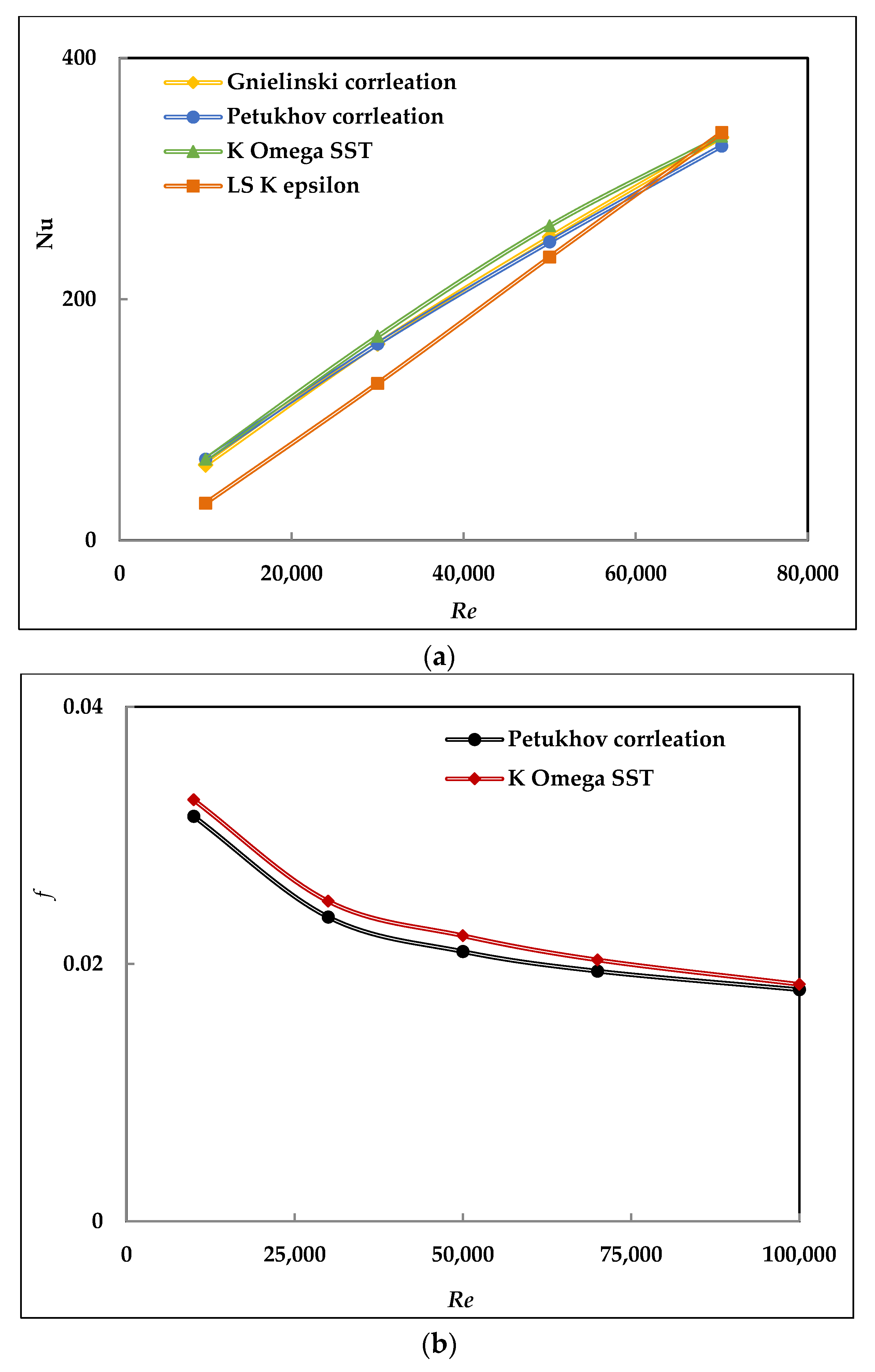
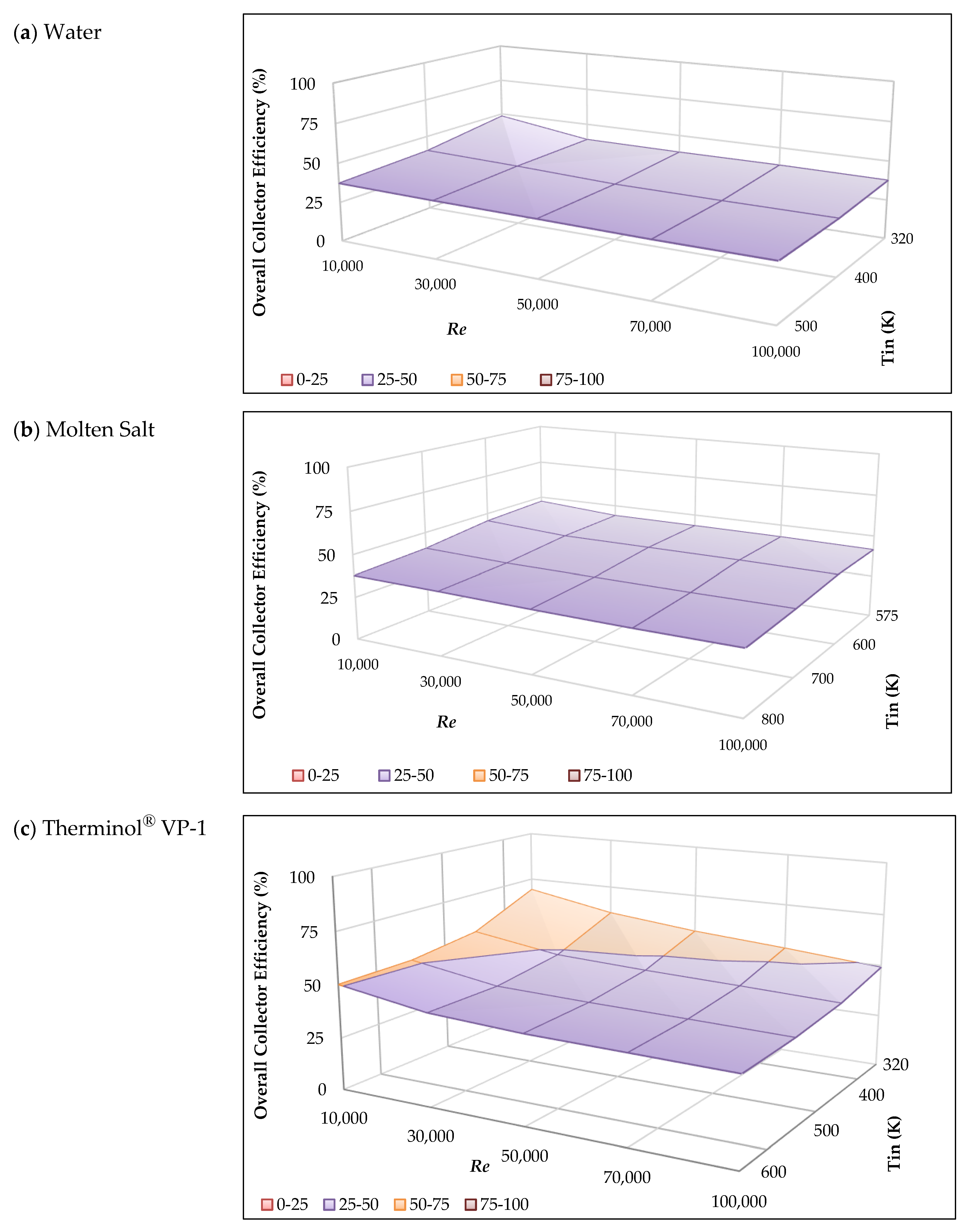
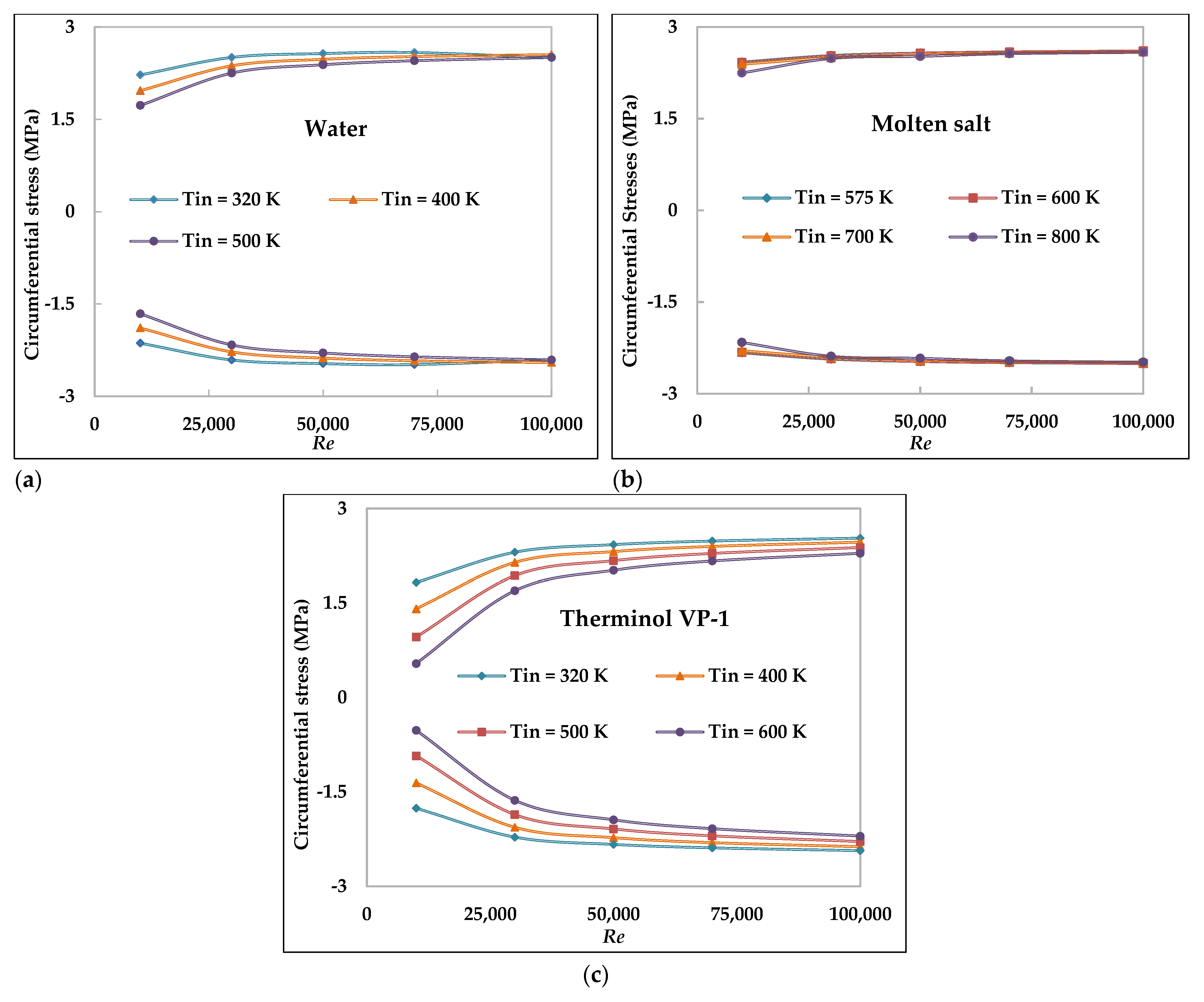
Thermal and hydraulic performances of the bare parabolic trough collectors were numerically investigated using three categorized-types of pure fluids; water, Therminol^® VP-1 and molten salt. The thermal performance parametric comparison using different pure fluids was also conducted considering the effect of various inlet temperatures and different $Re$ numbers. For the validation of two low-Reynolds turbulence models (Launder and Sharma (LS) k-epsilon and k-omega SST) were used taking into account different parameters; the overall thermal efficiency, the output fluid temperature, average $Nu$ number and average friction factor.

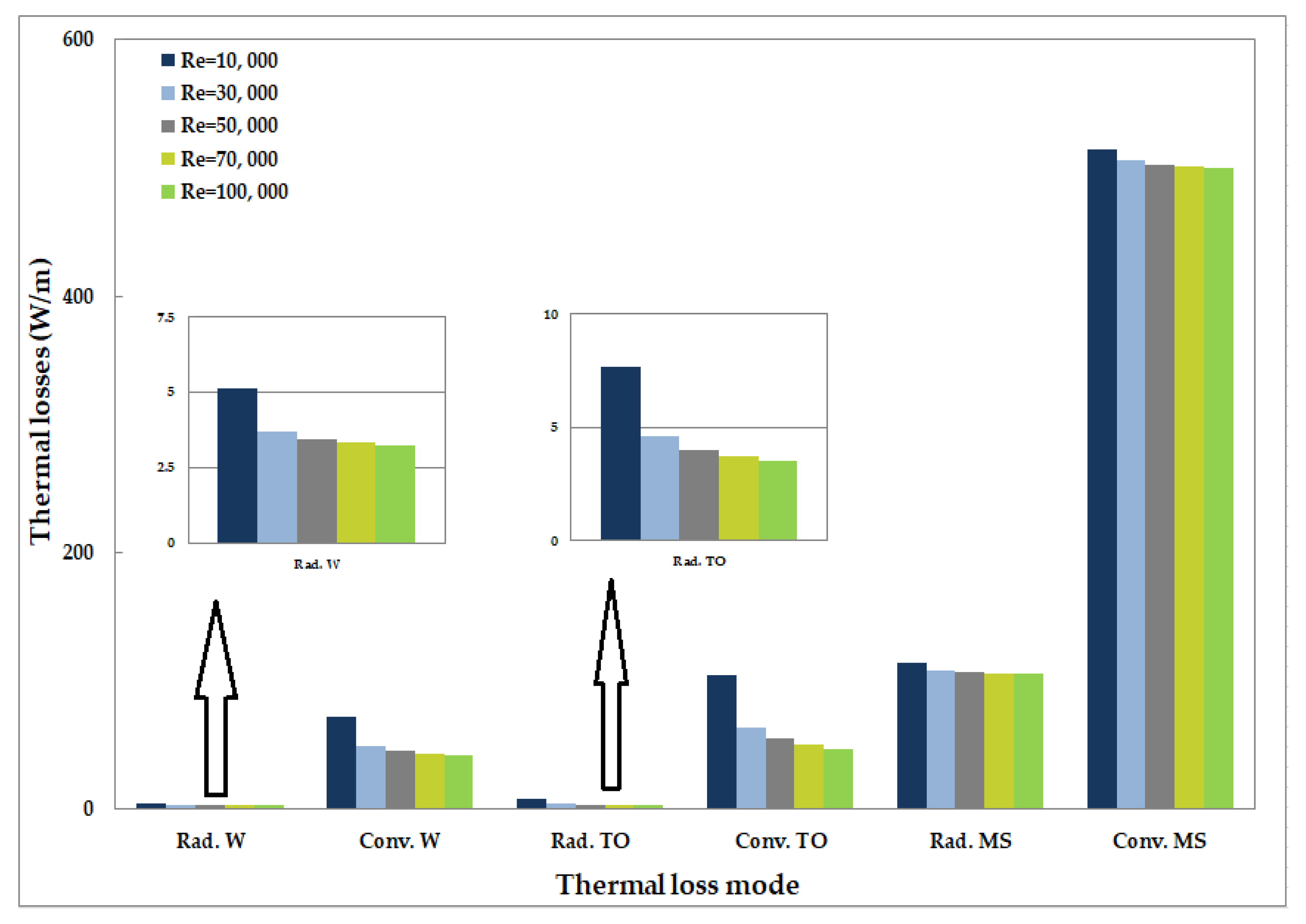
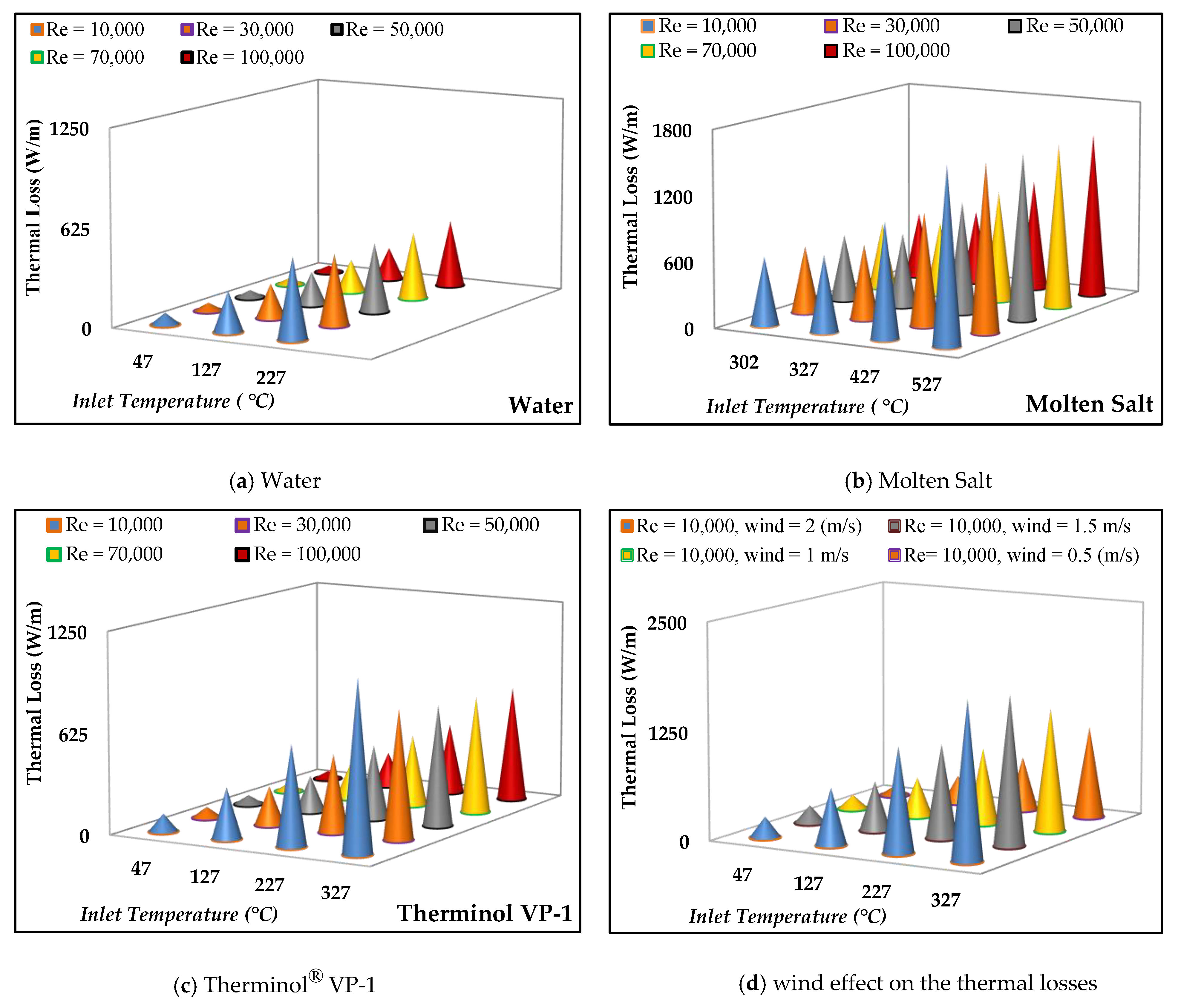
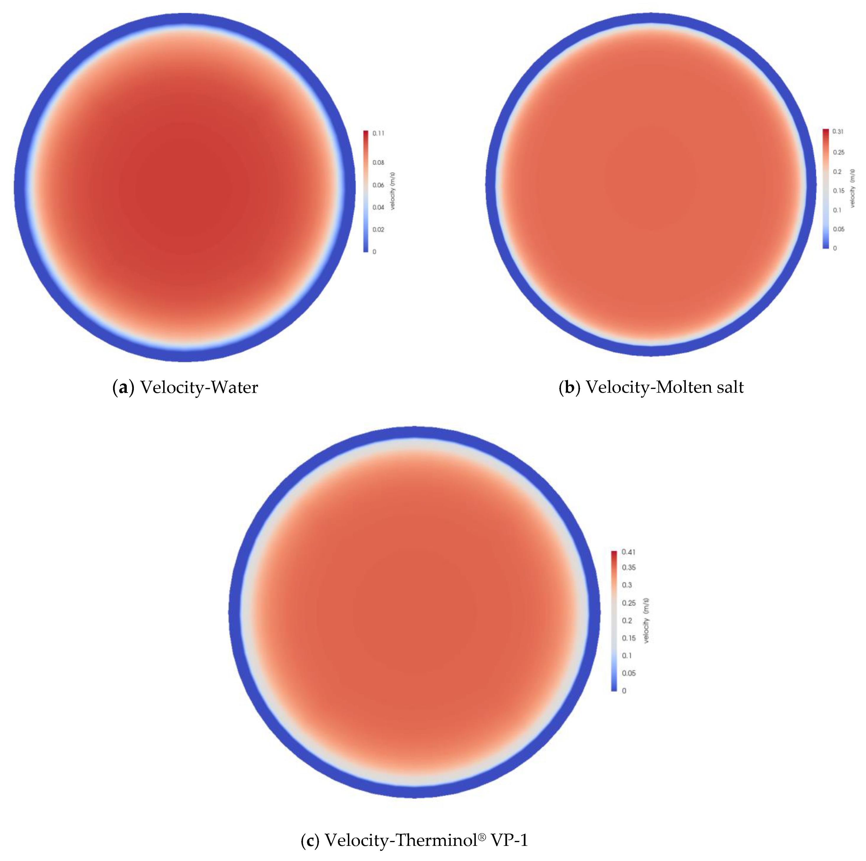
The validations showed that the k-omega SST model performed better when compared to both the experimental data and correlations. In order to assess the performance of each fluid, a number of parameters were investigated such as; average $Nu$ number, specific pressure drop distributions, thermal losses, thermal stresses in the circumferential direction of the absorber tube and overall thermal efficiency of the PTC. Results illustrated that for a temperature-range of (320–500) K, the Therminol^® VP-1 performed better than water and provided larger $Nu$ numbers, lower thermal stresses and higher thermal efficiency. However, for the common temperature-range between Therminol^® VP-1 and molten salt, both preformed more or less the same with lower thermal stresses in the case of Therminol^® VP-1. On the other hand, the molten salt was found to be the best choice for high operating temperatures (up to 873 K) since there was no significant reduction in the overall thermal efficiency at these high temperatures. Finally, the importance of results obtained in the current study illustrate comprehensively that the heat transfer behavior of the working fluid strongly depends upon the Prandtl number.

References

1. Blanco, M.J.; Miller, S. Introduction to Concentrating Solar Thermal (CST) Technologies, Advances in Concentrating Solar Thermal Research and Technology; Elsevier Inc.: Amsterdam, The Netherlands, 2017. [Google Scholar]
2. Abed, N.; Afgan, I. An Extensive Review of Various Technologies for Enhancing the Thermal and Optical Performances of Parabolic Trough Collectors. Int. J. Energy Res. 2020, 44, 5117–5164. [Google Scholar] [CrossRef] [Green Version]
3. Abed, N.; Afgan, I. Enhancement Techniques of Parabolic Trough Collectors: A Review of Past and Recent Technologies. Adv. Civ. Eng. Technol. 2019, 33, 313–318. [Google Scholar]
4. Sarafraz, M.M.; Arjomandi, M. Demonstration of plausible application of gallium nano-suspension inmicrochannel solar thermal receiver: Experimental assessment of thermo-hydraulic performance of microchannel. Int. Commun. Heat Mass Transf. 2018, 94, 39–46. [Google Scholar] [CrossRef]
5. Sarafraz, M.M.; Tlili, I.; Abdul Baseer, M.; Safaei, M.R. Potential of Solar Collectors for Clean Thermal Energy Production in Smart Cities using Nanofluids: Experimental Assessment and Efficiency Improvement. Appl. Sci. 2019, 9, 1877. [Google Scholar] [CrossRef] [Green Version]
6. Sarafraz, M.M.; Tlili, I.; Tian, Z.; Safaei, M.R. Smart optimization of a thermosyphon heat pipe for an evacuated tube solar collector using response surface methodology (RSM). Physica A 2019, 534, 1–11. [Google Scholar] [CrossRef]
7. Sarafraz, M.M.; Safaei, M.R. Diurnal thermal evaluation of an evacuated tube solar collector (ETSC) charged with graphene nanoplatelets-methanol nano-suspension. Renew. Energy 2019, 142, 364–372. [Google Scholar] [CrossRef]
8. Mwesigye, A.; Josua, P.M. Optimal Thermal and Thermodynamic Performance of a Solar Parabolic Trough Receiver with Different Nanofluids and at Different Concentration Ratios. Appl. Energy 2017, 193, 393–413. [Google Scholar] [CrossRef] [Green Version]
9. Bellos, E.; Christos, T. Parametric Investigation of Nanofluids Utilization in Parabolic Trough Collectors. Therm. Sci. Eng. Prog. 2017, 2, 71–79. [Google Scholar] [CrossRef]
10. Abed, N.; Afgan, I.; Nasser, A.; Iacovides, H.; Cioncolini, A.; Meakhail, T. Numerical Investigations of parabolic trough collectors using different nanofluids. In Proceedings of the 5th International Conference on Energy Engineering, Aswan, Egypt, 24–26 December 2019. [Google Scholar]
11. Bozorg, M.V.; Doranehgard, M.H.; Kun, H.; Qingang, X. Cfd Study of Heat Transfer and Fluid Flow in a Parabolic Trough Solar Receiver with Internal Annular Porous Structure and Synthetic Oil-Al2O3 Nanofluid. Renew. Energy 2020, 145, 2598–2614. [Google Scholar] [CrossRef]
12. Nahhas, T. Materials and Thermal Storage Systems by Sensible Heat for Thermodynamic Electro-Solar Plants. Ph.D. Thesis, University of Perpignan, Perpignan, France, 2017. [Google Scholar]
13. Odeh, S.D.; Morrison, G.L.; Behnia, M. Modelling of Parabolic Trough Direct Steam Generation Solar Collectors. Sol. Energy 1998, 62, 395–406. [Google Scholar] [CrossRef]
14. Forristall, R.E. Heat Transfer Analysis and Modeling of a Parabolic Trough Solar Receiver Implemented in Engineering Equation Solver; National Renewable Energy Laboratory: Golden, CO, USA, 2003.
15. Ouagued, M.; Khellaf, A. Simulation of the Temperature and Heat Gain by Solar Parabolic Trough Collector in Algeria. Int. J. Math. Comput. Phys. Electr. Comput. Eng. 2012, 6, 746–752. [Google Scholar]
16. Biencinto, M.; Rocío Bayón, E.; Lourdes, G. Simulation and Assessment of Operation Strategies for Solar Thermal Power Plants with a Thermocline Storage Tank. Sol. Energy 2014, 103, 456–472. [Google Scholar] [CrossRef]
17. Muñoz-Anton, J.; Biencinto, M.; Zarza, E.; Díez, L.E. Theoretical Basis and Experimental Facility for Parabolic Trough Collectors at High Temperature Using Gas as Heat Transfer Fluid. Appl. Energy 2014, 135, 373–381. [Google Scholar] [CrossRef]
18. Good, P.; Zanganeh, G.; Ambrosetti, G.; Barbato, M.C.; Pedretti, A.; Steinfeld, A. Towards a Commercial Parabolic Trough Csp System Using Air as Heat Transfer Fluid. Energy Proc. 2014, 49, 381–385. [Google Scholar] [CrossRef] [Green Version]
19. Wang, Y.; Qibin, L.; Lei, J.; Hongguang, J. A Three-Dimensional Simulation of a Parabolic Trough Solar Collector System Using Molten Salt As Heat Transfer Fluid. Appl. Therm. Eng. 2014, 70, 462–476. [Google Scholar] [CrossRef]
20. Selvakumar, P.; Somasundaram, P.; Thangavel, P. Performance Study on Evacuated Tube Solar Collector Using Therminol D-12 As Heat Transfer Fluid Coupled with Parabolic Trough. Energy Convers. Manag. 2014, 85, 505–510. [Google Scholar] [CrossRef]
21. Tahtah, R.; Ali, B.; Cherifa, A.; Mahfoud, K.; Fouzia, B. Experimental Study of Heat Transfer in Parabolic Trough Solar Receiver: Using Two Different Heat Transfer Fluids. AIP Conf. Proc. 1814, 1, 2017. [Google Scholar]
22. Bellos, E.; Korres, D.; Tzivanidis, C.; Antonopoulos, K.A. Design, Simulation and Optimization of a Compound Parabolic Collector. Sustain. Energy Technol. Assess. 2016, 16, 53–63. [Google Scholar]
23. Islam, M.K.; Hasanuzzaman, M.; Rahim, N.A. Modelling and Analysis of the Effect of Different Parameters on a Parabolic-Trough Concentrating Solar System. RSC Adv. 2015, 5, 36540–36546. [Google Scholar] [CrossRef]
24. Bellos, E.; Korres, D.; Tzivanidis, C.; Antonopoulos, K.A. A Detailed Working Fluid Investigation for Solar Parabolic Trough Collectors. Appl. Therm. Eng. 2017, 114, 374–386. [Google Scholar] [CrossRef]
25. Aguilar, R.; Valenzuela, L.; Avila-Marin, A.L.; Garcia-Ybarra, P.L. Simplified Heat Transfer Model for Parabolic Trough Solar Collectors Using Supercritical CO2. Energy Convers. Manag. 2019, 196, 807–820. [Google Scholar] [CrossRef]
26. Vutukuru, R.; Pegallapati, A.S.; Maddali, R. Suitability of Various Heat Transfer Fluids for High Temperature Solar Thermal Systems. Appl. Therm. Eng. 2019, 159, 1–9. [Google Scholar] [CrossRef]
27. Arslan, F.M.; Günerhan, H. Investigation of Energetic and Exergetic Performances of Parabolic Trough Collector with Using Different Heat Transfer Fluids. In E3S Web of Conferences; EDP Sciences: Les Ulis, France, 2019; Volume 111. [Google Scholar]
28. Duffie, J.A.; Beckman, W.A. Solar Engineering of Thermal Processes; John Wiley & Sons: Hoboken, NJ, USA, 2013. [Google Scholar]
29. Wirz, M.; Jules, P.; Andreas, H.; Aldo, S. Potential Improvements in the Optical and Thermal Efficiencies of Parabolic Trough Concentrators. Sol. Energy 2014, 107, 398–414. [Google Scholar] [CrossRef]
30. Bergman, T.L.; Incropera, F.P.; DeWitt, D.P.; Lavine, A.S. Fundamentals of Heat and Mass Transfer, 6th ed.; John Wiley & Sons: Hoboken, NJ, USA, 2006. [Google Scholar]
31. Bhowmik, N.C.; Mullick, S.C. Calculation of Tubular Absorber Heat Loss Factor. Sol. Energy 1985, 35, 219–225. [Google Scholar] [CrossRef]
32. Dudley, V.E.; Kolb, G.J.; Sloan, M.; Keamey, D. Test Results: SEGS LS-2 Solar Collector. SAND94-1884; Sandia National Labs.: Albuquerque, NM, USA, 1994; pp. 1–12. [Google Scholar]
33. Swinbank, W.C. Long-wave radiation from clear skies. Q. J. R. Meteorol. Soc. 1963, 89, 339–348. [Google Scholar] [CrossRef]
34. Petukhov, B.S. Heat Transfer and Friction in Turbulent Pipe Flow with Variable Physical Properties. Adv. Heat Transf. 1970, 6, 503–564. [Google Scholar]
35. Gnielinski, V. New Equations for Heat and Mass Transfer in Turbulent Pipe and Channel Flow. Int. Chem. Eng. 1976, 16, 359–368. [Google Scholar]
36. Mwesigye, A.; Zhongjie, H.; Meyer, J.P. Thermal Performance and Entropy Generation Analysis of a High Concentration Ratio Parabolic Trough Solar Collector with Cu-Therminol®vp-1 Nanofluid. Energy Convers. Manag. 2016, 120, 449–465. [Google Scholar] [CrossRef] [Green Version]
37. Pacheco, J.E.; Ralph, M.E.; Chavez, J.M.; Dunkin, S.R.; Rush, E.E.; Ghanbari, C.M.; Matthews, M.W. Results of Molten Salt Panel and Component Experiments for Solar Central Receivers: Cold Fill, Freeze/Thaw, Thermal Cycling and Shock, and Instrumentation Tests; Sandia National Labs.: Albuquerque, NM, USA, 1995. [Google Scholar]
38. Launder, B.E.; Sharma, B.I. Application of the energy-dissipation model of turbulence to the calculation of flow near a spinning disc. Lett. Heat Mass Transf. 1974, 11, 131–137. [Google Scholar]
39. Menter, F.R. Two-equation eddy-viscosity turbulence models for engineering applications. AIAA J. 1994, 32, 1598–1605. [Google Scholar] [CrossRef] [Green Version]
40. Van Leer, B. Towards the ultimate conservative difference scheme. II. Monotonicity and conservation combined in a second-order scheme. J. Comput. Phys. 1974, 14, 361–370. [Google Scholar] [CrossRef]
41. Issa, R.I. Solution of the implicitly discretised fluid flow equations by operator-splitting. J. Comput.Phys. 1986, 62, 40–65. [Google Scholar] [CrossRef]
42. Barron, B.R.; Barron, R.F. Design for Thermal Stresses; John Wiley & Sons: Hoboken, NJ, USA, 2013. [Google Scholar]
43. Benoit, H.; Spreafico, L.; Gauthier, D.; Flamant, G. Review of Heat Transfer Fluids in Tube-Receivers Used in Concentrating Solar Thermal Systems: Properties and Heat Transfer Coefficients. Renew. Sustain. Energy Rev. 2016, 55, 298–315. [Google Scholar] [CrossRef]
44. Kaloudis, E.; Papanicolaou, E.; Belessiotis, V. Numerical Simulations of a Parabolic Trough Solar Collector with Nanofluid Using a Two-Phase Model. Renew. Energy 2016, 97, 218–229. [Google Scholar] [CrossRef]
Figure 1. The typical configuration of cross-section of a PTC system.
Energies 13 03776 g001
Figure 2. Three dimensional hexahedral meshes used in this study.
Energies 13 03776 g002
Figure 3. Mesh independence study for three different grids used in the present study.
Energies 13 03776 g003
Figure 4. Validation of the present study with the thermal efficiency data of Dudley et al. [24].
Energies 13 03776 g004
Figure 5. Comparisons between the present work with the experimental correlations (a) Average Nusselt number correlations proposed by Petukhov [34] and Gnielinski [35] (b) Friction factor, f, correlation proposed by Petukhov [34].
Energies 13 03776 g005
Figure 6. Nusselt number profiles of different fluids used in the present work.
Energies 13 03776 g006
Figure 7. The specific pressure drop profiles of all fluids under consideration.
Energies 13 03776 g007
Figure 8. Convection and radiation thermal losses at different R e numbers at the smallest inlet temperatures of different fluids; W (Water), T (Therminol® VP-1) and MS (Molten Salt).
Energies 13 03776 g008
Figure 9. Thermal losses behaviour of all fluids used in this study.
Energies 13 03776 g009
Figure 10. Thermal efficiency behaviour of all heat transfer fluids under different parameters.
Energies 13 03776 g010
Figure 11. Thermal stresses distributions of all working fluids at different inlet fluid temperatures.
Energies 13 03776 g011
Figure 12. Velocity contours of all fluids at the smallest inlet temperatures.
Energies 13 03776 g012
Figure 13. Temperature contours of all fluids at the smallest inlet temperatures.
Energies 13 03776 g013
Figure 14. Temperature profiles of all working fluids used in the current study.
Energies 13 03776 g014