Performance Assessment of Large Photovoltaic (PV) Plants Using an Integrated State-Space Average Modeling Approach

Abstract

Distributed power converters represent a technical solution to improve the performance of large or utility-scale photovoltaic (PV) plants. Unfortunately, evaluation of the yield obtained in large PV fields by using distributed converters is a difficult task because of recurring partial unavailability, inaccuracy of power analyzers, operating constraints imposed by the Power Plant Controller and so on. To overcome such issues in real operating scenarios, a new modeling strategy has been introduced and validated in terms of computational complexity and accuracy. This approach is based on the state-space averaging technique which is applied to large PV plants with multiple conversion stages by performing some elaborations in order to get a final integrated model. The new modeling strategy has been tested in MatLab Simulink environment using data coming from a 300 MW PV plant located in Brazil representing the case study of this work. In this plant, one subfield is equipped with central inverters while another is with string inverters. The proposed model, whose accuracy is in the range from 2.2 to 2.7% with respect to the measured energy, effectively supports data analysis leading to a consistent performance assessment for the distributed conversion system. Final results highlight that string inverters ensure a gain of about 2% in terms of produced energy.

1. Introduction

Distributed power converters in PV fields play a key role in the solar industry for new constructions and for retrofitting activities as well. Many tests are carried out in laboratory as well as in small size and medium size PV plants with the purpose to compare the performance of string and central inverters. Some examples are reported in papers [1,2,3,4]. On the contrary, in literature a comprehensive analysis about test results for large PV plants is missing.

A first reason for this lack of information deals with the low number of large PV fields using distributed converters. In fact, installation of central inverters is actually the most common option for large plants. At the same time, the number of plants with distributed converters is growing fast. In most cases, installation of distributed converters is aimed to get energy recovery related to mismatch losses occurring in case of non-uniform aging of PV modules, tracker faults and so on [5].

Focusing on performance evaluation for long time periods in large PV fields, some issues often occur in big data analysis. In fact, monitoring system can be affected by faults in dataloggers and sensors leading to missing or wrong data. More generally, the number of unavailabilities is expected to be quite high because of the high number of components in which a fault can occur. Moreover, in some cases there are additional operating constraints to take into account, for example thresholds set by the power plant controller (PPC) or by the inverters fixing the maximum power that a PV subfield can deliver to grid.

These problems can be solved by exploiting suitable models able to track the expected behavior of the PV plant in any operating conditions while filling the gaps due to faults and missing data.

Many papers deal with modeling and simulation of PV plants [6,7,8,9,10,11,12,13]. Unfortunately, almost all these papers investigate on small or medium size PV plants. They often focus on modeling of PV modules [6,7,8,9]. In other cases, focus is on converters operation, frequently target is to set a proper control strategy [10,11,12,13].

Generally, modeling approach and simulation platform for large or utility-scale PV plants are chosen on the basis of specific analysis targets taking into account requirements in terms of acceptable computational effort. If target is the yield estimation for a long time period, modeling of power converters is usually neglected in order to limit the computational effort. In this case, converters are replaced by functional blocks considering only the efficiency value [14,15]. On the contrary, if some specific operating conditions need to be investigated including details on converters operation and losses, accurate models need to be implemented [16]. In the latter case, computational effort could be very high. Under this perspective, in case of energy assessment analysis for months or years, detailed models cannot be exploited to simulate the behaviour of a large PV system having thousands of modules and hundreds of distributed converters.

Some authors tried to overcome these limitations by introducing simplified modeling approaches usually known as behavioural models. For example, model presented in [14] simulates the electrical behaviour of commercial grid-connected PV inverters in accordance with regulations on power quality. Simulation results show the waveform of injected AC current in case of power dynamics or grid voltage disturbances. In [17] a non-parametric approach is used to evaluate the energy delivered to grid by six PV fields creating a forecast method by means of meteorological variables.

Although behavioural approaches fulfill the requirement of low computational burden, the actual physical configuration of the PV system could be completely neglected. In some cases, this is a relevant drawback. For example, if the performance analysis aims to evaluate losses over time in DC and AC cables, some technical details about converters (e.g., their topology and control strategy) are strictly necessary to calculate voltage and current values in both DC side and AC side. In many real PV plants, electrical quantities in some sections of the conversion system are not acquired by dataloggers, consequently an accurate estimation of losses is impossible.

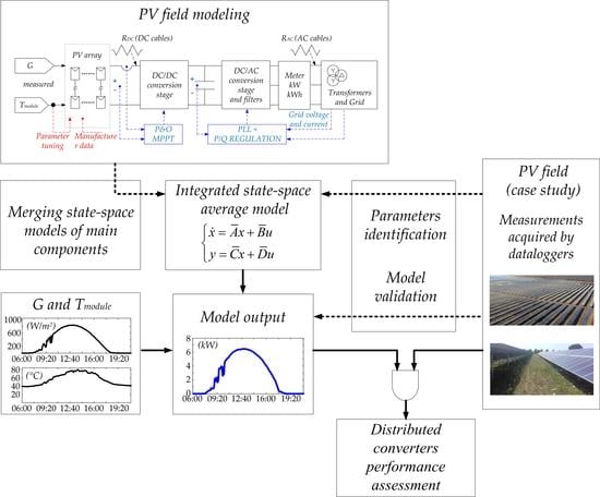
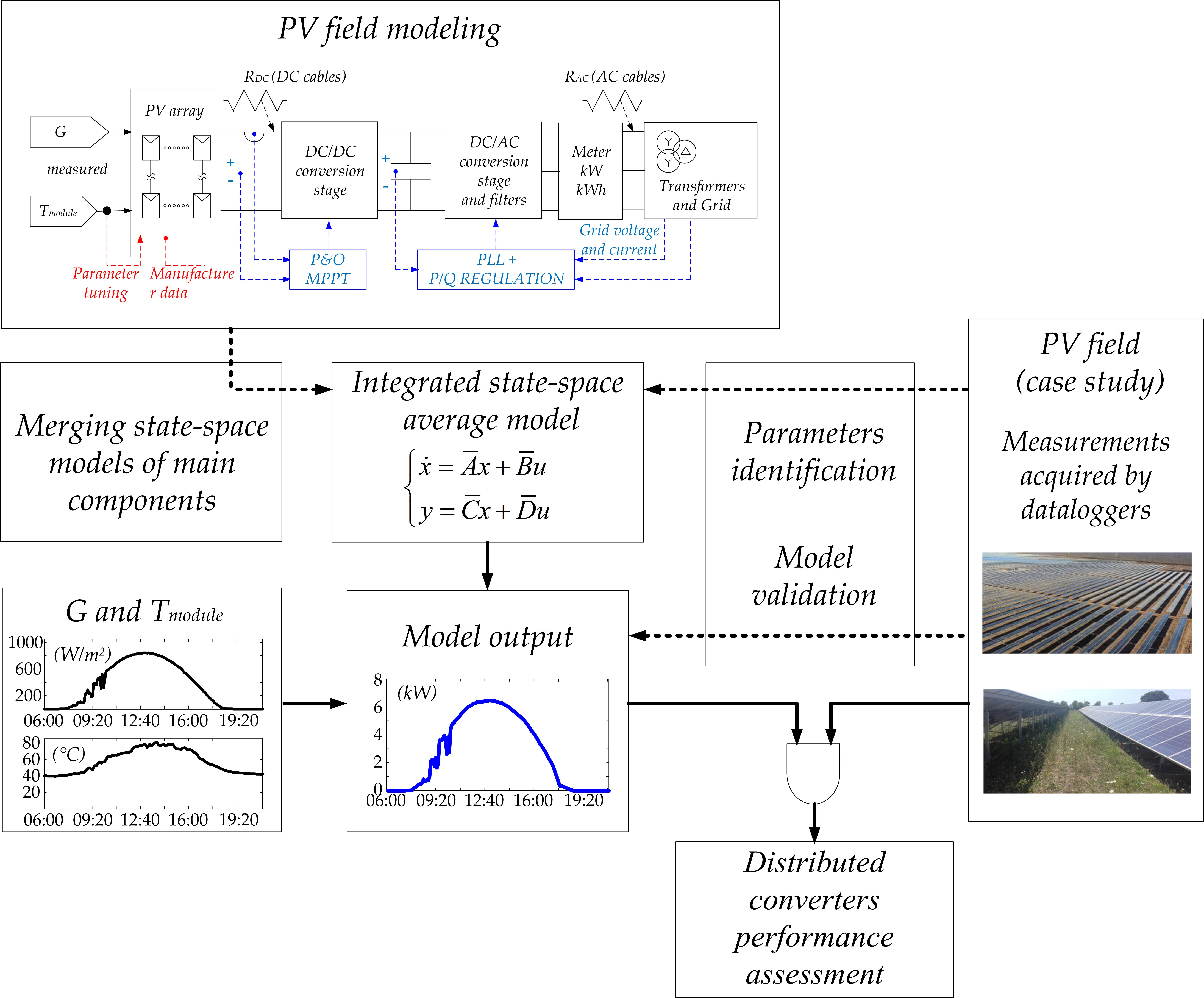
The behavioural model described in this paper consists of an integrated state-space average model. The latter computes all the electrical quantities in each section of a PV plant. In such a way, it is possible to calculate losses, voltage drops, etc. Satisfactory accuracy is obtained while large computational effort is avoided. The advantages of the proposed approach are listed here:

• Significant reduction of simulation time, see Section 4.2
• Basic model structure can be easily adapted to different system configurations (e.g., central inverters, string inverters, string optimizers combined with central inverters, etc.) performing minimal modifications
• Several common identification methods can be used to identify parameters being part of the state-space representation of the PV system
• Technical details about converters (e.g., their topology and control strategy) become no longer necessary. Furthermore, in many cases such information are covered by policies on industrial secrets
• Behavioural model can be easily integrated in monitoring systems and exploited for forecasting purposes and for fault detection
• The proposed state-space model can be implemented in any simulation platform

The introduced model has been validated in terms of computational complexity and accuracy. It has been applied to a specific case study represented by the performance comparison between central and string converters installed in two different PV subfields which form a 5 MW experimental cluster of a 300 MW PV plant located in Brazil. Comparison criteria deal with energy production. Data analysis is supported by the proposed model developed in the MatLab/Simulink environment. The case study is briefly described in Section 2. Our modeling approach is introduced in Section 3 providing information on integrated state-space average method, parameters identification and control system. Section 4 reports model validation in terms of accuracy and computational effort. Section 5 describes the implementation of the introduced model for the case study. The same Section shows the aggregate results regarding the performance assessment of distributed converters.

2. Case Study

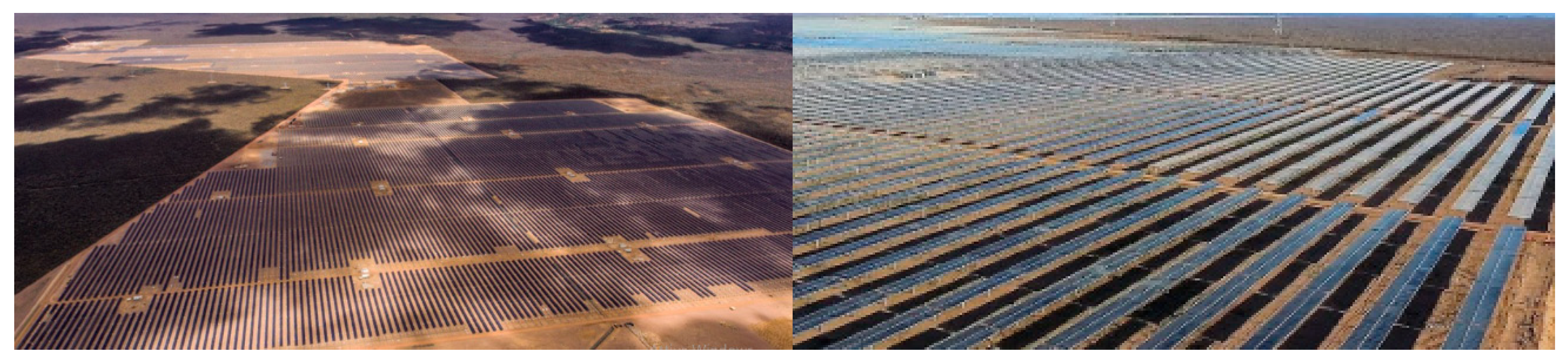
Figure 1 shows two pictures of the 300 MW PV plant representing the case study of this paper. PV field is connected to the 34.5 kV 60 Hz grid using power transformers, one for each 2.5 MW subfield. PV modules are mounted on horizontal single-axis tracking systems.

A 5 MW cluster was realized for testing purpose with the objective to compare the performance of central inverters and string inverters manufactured by international companies.

In the 2.5 MW subfield with central converters there are two inverters whose rated power is 1025 kVA, fan cooled, mounted into an electric cabin. The actual AC power reaches about 1045 kVA in case of unity power factor.

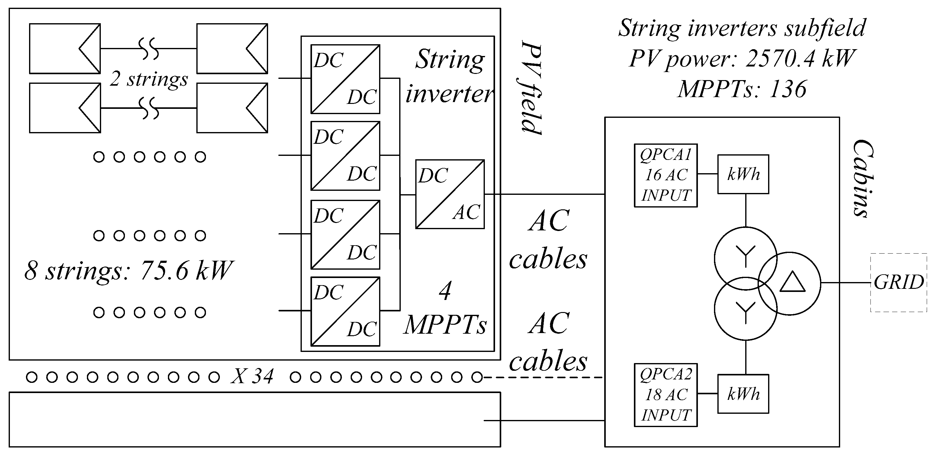
In the 2.5 MW subfield with string inverters each converter has a rated power of 60 kVA. Thanks to a particular design, maximum power rises up to 66 kVA in case of unity power factor (66 kW) and of ambient temperature below 30 °C. String converters, mounted into the field without using cabinets and without fan cooling, are grouped in a cabin close to transformers using AC parallel switchboards named QPCA.

The number of PV modules connected to each conversion system is exactly the same (total DC rated power is 2570.4 kW for both subfields) so that comparison is performed in the same conditions. PV strings are composed of 30 PV modules in series. Rated power of modules is 315 W. There are 272 strings in each subfield, 136 for each central inverter and 8 for each string inverter.

The configuration of subfields under test is represented in Figure 2 and Figure 3. Technical data for the main power components are given in

Table 1. Technical specifications for the main power components.

PV Modules		Central Inverters
Pmodule (W)	315	Rated AC power (kVA)	1025
Voc (V)	46.2	AC output (V, Hz)	400 ± 10%, 50/60
Isc (A)	9.01	MPPT DC voltage range (V)	675–1320
VMPP (V)	37.2	Maximum Efficiency (%)	98.9
IMPP (A)	8.48	MPPTs per power converter	1
NOCT (°C)	45 ± 2	String Inverters
Pmodule/Tmodule (%/°C)	−0.40	Rated AC power (kVA)	60 (up to 66)
Voc/Tmodule (%/°C)	−0.30	AC output (V, Hz)	800, 50/60
Isc/Tmodule (%/°C)	+0.06	MPPT DC voltage range (V)	600–1450
Cells	Poly	Maximum Efficiency (%)	99.0
Number of cells	72	MPPTs per power converter	4

.

System monitoring is realized using global irradiance sensors mounted on trackers, ambient temperature sensors, module temperature sensors, inverter temperature sensors, power analyzers and power meters. Energy flowing in central inverters is measured by a meter connected to voltage and current sensors placed at the AC side of inverters. In subfields with string inverters a meter provides the value of AC energy. At the DC side, string monitoring is embedded in each converter. Accuracy of data provided by the monitoring system can be assumed in the range 2.0–2.5%. The criterion selected for the performance assessment of distributed converters is basically the average gain in terms of energy produced by using string inverters with respect to central inverters.

3. Large PV Fields Modeling

3.1. Modeling Approach

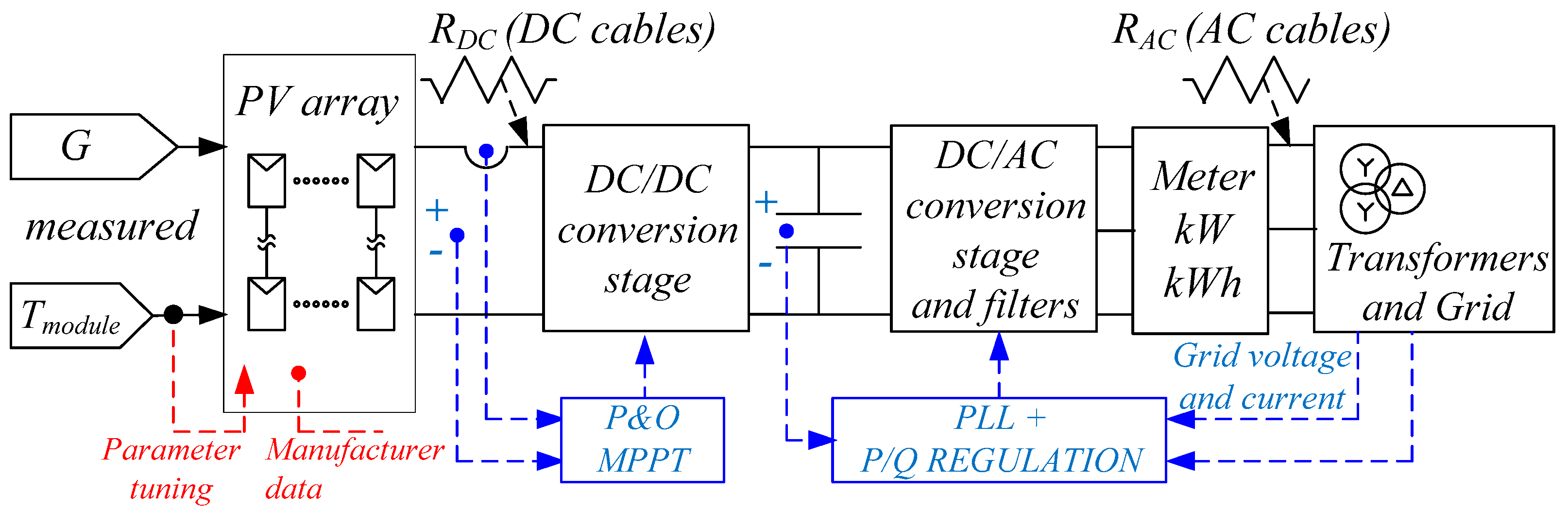
A generic representation of a large PV plant is shown in Figure 4. This basic configuration can be adapted to simulate PV fields with central inverters as well as the ones with string inverters or with power optimizers at module or string level. Moreover, it is suitable for the whole PV plant under investigation or for a specific subfield (strings, string boxes, etc.) by performing minimal modifications.

About the implementation of this kind of model in a simulation platform, it is possible to distinguish three main approaches:

• Detailed models, in this case each component (array, converter, grid, etc.) is inserted in simulation considering its physical description, circuit topology and operation mode. For example, converters are modeled reproducing their detailed topology and their switching modulation technique [16]
• Models in which physical description of components is neglected [17]
• Intermediate models, which are a trade-off between the previous categories [14]

The behavioural model introduced in this work belongs to the third category. It is based on a modified state-space averaging model which has been selected following the primary target to get a simplified representation for the multi-stage conversion system of large PV fields with distributed converters. In fact, in this circumstance there are usually both DC-DC converters (e.g., first stage of string inverters or power optimizers) and DC-AC converters (grid connected inverters, usually multilevel inverters).

Models of power converters for PV applications are designed in different ways. In the case of stringent requirements on computational effort for energy assessment in a long-term time horizon, the common approach to model DC-DC converters and their control system is the state-space averaging method, some examples are in [18,19,20]. Grid connected inverters are usually modeled using relationships coming from energy balances [14,19,21] or from equivalent circuits [10]. In the latter case, electrical quantities are sometimes expressed as phasors [22,23].

In the literature there is a lack of information about integrated modeling approaches able to represent multiple conversion stages in large PV fields. This work contributes to fill this gap. In fact, the main novelty is related to the creation of a complete model in which each component of the PV field is included using its state-space representation. Integration of different conversion stages is obtained thanks to the development of a direct way for the analytical calculation of current flowing in the DC-link.

All the components of the generation and conversion system are mixed into a single state-space average model obtaining an integrated representation for the entire PV system. In other words, the PV plant becomes a single state-space system. Inputs of such system are irradiance and cell temperature while outputs are the energy production and all the electric quantities in every part of the system.

3.2. Conversion System: Basic Converter Models

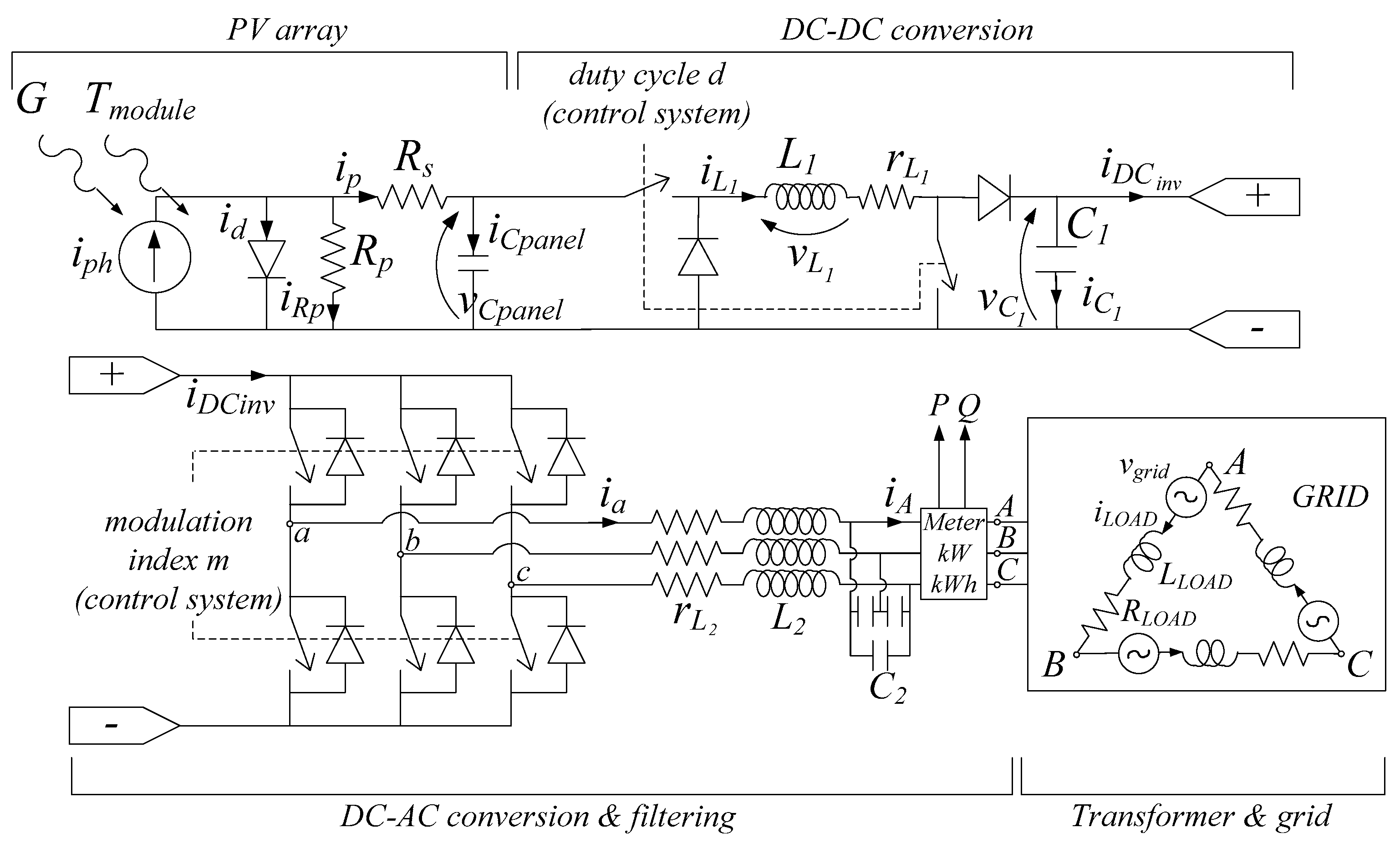
This section refers to a specific multi-stage topology, represented in Figure 5. Such topology has been chosen to better explain the modeling approach.

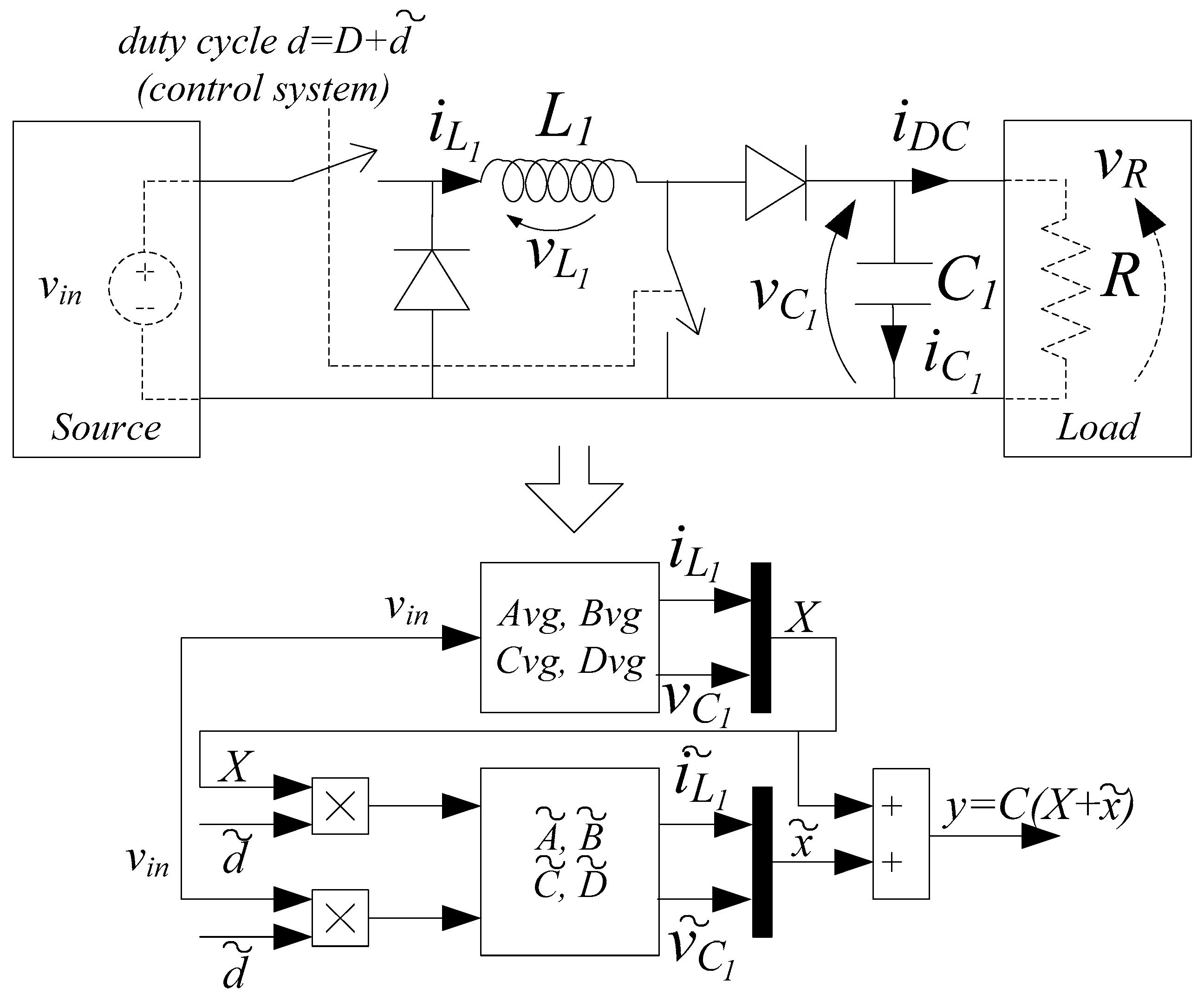
Focusing on the DC-DC converter stage and representing the same as a single block with a fictitious voltage source v_in and a fictitious load R as in Figure 6, its state-space average form is obtained following the well-known procedure for which ON and OFF states have to be analyzed separately by building Kirchhoff equations for state variables and then mixed together to obtain the final average state-space system. An example is discussed in [18].

Variation of duty cycle d controlled by the MPPT algorithm can be modeled as a perturbation $\tilde{d}$ superimposed to the steady-state duty cycle D [20]. The basic form of a state-space average model is in Equation (1):

$$\{\begin{array}{l}\dot{X}={\overline{A}}_{DC}X+{\overline{B}}_{DC}u\\ Y={\overline{C}}_{DC}X+{\overline{D}}_{DC}u\end{array}$$

(1)

where:

$${\overline{A}}_{DC}=A_{D{C}_{ON}}d+A_{D{C}_{OFF}}\left(1-d\right)A_{D{C}_{ON}}=\left[\begin{array}{cc}0& 0\\ 0& -\frac{1}{R{C}_1}\end{array}\right]A_{D{C}_{OFF}}=\left[\begin{array}{cc}0& -\frac{1}{L_1}\\ \frac{1}{C_1}& -\frac{1}{R{C}_1}\end{array}\right]$$

(2)

$${\overline{B}}_{DC}=B_{D{C}_{ON}}d+B_{D{C}_{OFF}}\left(1-d\right)B_{D{C}_{ON}}=\left[\begin{array}{c}\frac{1}{L_1}\\ 0\end{array}\right]B_{D{C}_{OFF}}=\left[\begin{array}{c}0\\ 0\end{array}\right]$$

(3)

$${\overline{C}}_{DC}=C_{D{C}_{ON}}=C_{D{C}_{OFF}}=\left[\begin{array}{cc}1& 0\\ 0& 1\end{array}\right]{\overline{D}}_{DC}\mathrm{null}$$

(4)

The extension of this state-space system, in presence of $\tilde{d}$, is:

$$\{\begin{array}{l}\tilde{\dot{x}}={\overline{A}}_{DC}\tilde{x}+{\displaystyle [}{\displaystyle (}{A}_{D{C}_{ON}}-A_{D{C}_{OFF}}{\displaystyle )}{\displaystyle (}{B}_{D{C}_{ON}}-B_{D{C}_{OFF}}{\displaystyle )}{\displaystyle ]}{\displaystyle [}\begin{array}{c}X\tilde{d}\\ v_{in}\tilde{d}\end{array}{\displaystyle ]}\\ \tilde{y}={\overline{C}}_{DC}\tilde{x}+\left[\left(C_{D{C}_{ON}}-C_{D{C}_{OFF}}\right)X\right]\tilde{d}={\overline{C}}_{DC}\tilde{x}\end{array}$$

(5)

$$u=U=v_{in}y=Y+\tilde{y}x=X+\tilde{x}d=D+\tilde{d}x=\left[\begin{array}{c}{i}_{L_1}\\ v_{C_1}\end{array}\right]$$

(6)

In this way, a simple state-space average system models the behavior of any DC-DC converter topology in presence of variations of duty cycle forced by the MPPT control system.

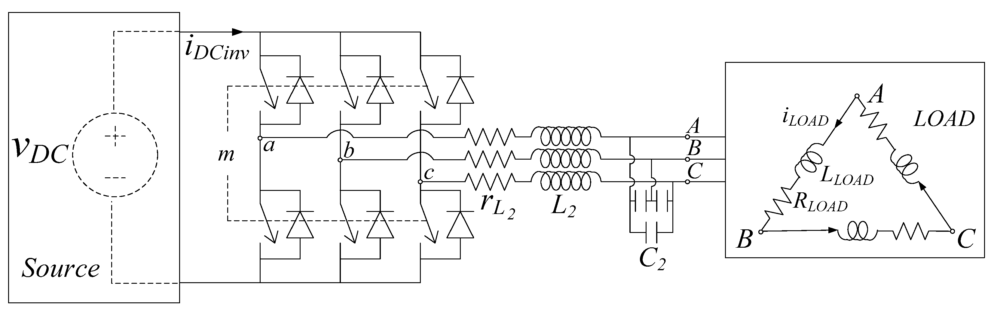
About the inverter and filtering stage in Figure 7, for sake of clarity in this section load is assumed to be three-phase inductive-resistive in delta connection without grid sources. Basic modeling approach is described in [23] exploiting a generalized state-space averaging method based on Fortescue symmetrical components and on Fourier transform.

The state-space form derives from Kirchhoff laws, similarly to what shown in [23]:

$$\{\begin{array}{l}\frac{d}{dt}\left[\begin{array}{c}{i}_{ab}\\ i_{bc}\\ i_{ca}\end{array}\right]=-\frac{r_{L_2}}{L_2}\left[\begin{array}{c}{i}_{ab}\\ i_{bc}\\ i_{ca}\end{array}\right]-\frac{1}{3L_2}\left[\begin{array}{c}{v}_{AB}\\ v_{BC}\\ v_{CA}\end{array}\right]+\frac{\sqrt{3}m}{6L_2}\left[\begin{array}{c}{v}_{DC}\cos \left(\omega t-{\phi }_a+\frac{\pi }{6}\right)\\ v_{DC}\cos \left(\omega t-{\phi }_b+\frac{\pi }{6}\right)\\ v_{DC}\cos \left(\omega t-{\phi }_c+\frac{\pi }{6}\right)\end{array}\right]\\ \frac{d}{dt}\left[\begin{array}{c}{v}_{AB}\\ v_{BC}\\ v_{CA}\end{array}\right]=\frac{1}{C_2}\left[\begin{array}{c}{i}_{ab}\\ i_{bc}\\ i_{ca}\end{array}\right]-\frac{1}{C_2}\left[\begin{array}{c}{i}_{LOA{D}_{AB}}\\ i_{LOA{D}_{BC}}\\ i_{LOA{D}_{CA}}\end{array}\right]\\ \frac{d}{dt}\left[\begin{array}{c}{i}_{LOA{D}_{AB}}\\ i_{LOA{D}_{BC}}\\ i_{LOA{D}_{CA}}\end{array}\right]=-\frac{R_{LOAD}}{L_{LOAD}}\left[\begin{array}{c}{i}_{LOA{D}_{AB}}\\ i_{LOA{D}_{BC}}\\ i_{LOA{D}_{CA}}\end{array}\right]+\frac{1}{L_{LOAD}}\left[\begin{array}{c}{v}_{AB}\\ v_{BC}\\ v_{CA}\end{array}\right]\end{array}$$

(7)

where i_ab, i_bc and i_ca are virtual line currents, m is the modulation index. The other parameters are shown in Figure 7.

The AC currents and voltages are represented as the sum of their Fortescue symmetrical components as follows:

$$\{\begin{array}{l}{i}_{ab}={\left(i_{ab}\right)}_{-1}{e}^{-j\omega t}+{\left(i_{ab}\right)}_0+{\left(i_{ab}\right)}_1{e}^{j\omega t}\\ i_{bc}={\left(i_{bc}\right)}_{-1}{e}^{-j\omega t}+{\left(i_{bc}\right)}_0+{\left(i_{bc}\right)}_1{e}^{j\omega t}\\ i_{ca}={\left(i_{ca}\right)}_{-1}{e}^{-j\omega t}+{\left(i_{ca}\right)}_0+{\left(i_{ca}\right)}_1{e}^{j\omega t}\\ v_{AB}={\left(v_{AB}\right)}_{-1}{e}^{-j\omega t}+{\left(v_{AB}\right)}_0+{\left(v_{AB}\right)}_1{e}^{j\omega t}\\ v_{BC}={\left(v_{BC}\right)}_{-1}{e}^{-j\omega t}+{\left(v_{BC}\right)}_0+{\left(v_{BC}\right)}_1{e}^{j\omega t}\\ v_{CA}={\left(v_{CA}\right)}_{-1}{e}^{-j\omega t}+{\left(v_{CA}\right)}_0+{\left(v_{CA}\right)}_1{e}^{j\omega t}\\ i_{LOA{D}_{AB}}={\left(i_{LOA{D}_{AB}}\right)}_{-1}{e}^{-j\omega t}+{\left(i_{LOA{D}_{AB}}\right)}_0+{\left(i_{LOA{D}_{AB}}\right)}_1{e}^{j\omega t}\\ i_{LOA{D}_{BC}}={\left(i_{LOA{D}_{BC}}\right)}_{-1}{e}^{-j\omega t}+{\left(i_{LOA{D}_{BC}}\right)}_0+{\left(i_{LOA{D}_{BC}}\right)}_1{e}^{j\omega t}\\ i_{LOA{D}_{CA}}={\left(i_{LOA{D}_{CA}}\right)}_{-1}{e}^{-j\omega t}+{\left(i_{LOA{D}_{CA}}\right)}_0+{\left(i_{LOA{D}_{CA}}\right)}_1{e}^{j\omega t}\end{array}$$

(8)

For each term, neglecting the presence of inverse and homopolar components as a first approximation, state variables are the real and imaginary parts of the direct component:

$$\{\begin{array}{l}{\left(i_{ab}\right)}_1=x_1+j{x}_2\\ {\left(i_{bc}\right)}_1=x_3+j{x}_4\\ {\left(i_{ca}\right)}_1=x_5+j{x}_6\\ {\left(v_{AB}\right)}_1=x_7+j{x}_8\\ {\left(v_{BC}\right)}_1=x_9+j{x}_{10}\\ {\left(v_{CA}\right)}_1=x_{11}+j{x}_{12}\\ {\left(i_{LOA{D}_{AB}}\right)}_1=x_{13}+j{x}_{14}\\ {\left(i_{LOA{D}_{BC}}\right)}_1=x_{15}+j{x}_{16}\\ {\left(i_{LOA{D}_{CA}}\right)}_1=x_{17}+j{x}_{18}\end{array}$$

(9)

The other components can be easily included as described in [23], if necessary. AC currents and voltages become:

$$\{\begin{array}{l}{i}_{ab}=2x_1\cos \omega t-2x_2\sin \omega t\\ i_{bc}=2x_3\cos \omega t-2x_4\sin \omega t\\ i_{ca}=2x_5\cos \omega t-2x_6\sin \omega t\\ v_{AB}=2x_7\cos \omega t-2x_8\sin \omega t\\ v_{BC}=2x_9\cos \omega t-2x_{10}\sin \omega t\\ v_{CA}=2x_{11}\cos \omega t-2x_{12}\sin \omega t\\ i_{LOA{D}_{AB}}=2x_{13}\cos \omega t-2x_{14}\sin \omega t\\ i_{LOA{D}_{BC}}=2x_{15}\cos \omega t-2x_{16}\sin \omega t\\ i_{LOA{D}_{CA}}=2x_{17}\cos \omega t-2x_{18}\sin \omega t\end{array}$$

(10)

Starting from these relationships, state-space equations of the DC-AC converter can be integrated in the PV plant model described in Section 3.6. Quantities (x₁,…,x₁₈) are state variables.

3.3. Analytical Calculation of DC-Link Current

From the description of conversion stages, merging of different modeling approaches becomes necessary to obtain a comprehensive representation for the entire PV system. The key parameter for obtaining such merging is the DC-link current i_DCinv.

Average or RMS value of this current is usually calculated from power balances [24] or from integral calculation [24,25]. In some cases the latter method is applied using a reduced-order Fourier transform. Computational effort related to data storage in integrals is the main drawback of these methods.

In this work, calculation of the average value of DC-link current has been developed in a direct way using the AC current components. To explain this achievement, starting point is this equation:

$$\begin{array}{l}{i}_{D{C}_{inv}}=s_a{i}_a+s_b{i}_b+s_c{i}_c=s_a{i}_{ab}-s_a{i}_{ca}+s_b{i}_{bc}-s_b{i}_{ab}+s_c{i}_{ac}-s_c{i}_{bc}=\\ =\left(s_a-s_b\right)i_{ab}+\left(s_b-s_c\right)i_{bc}+\left(s_c-s_a\right)i_{ca}\end{array}$$

(11)

where s is a function representing PWM modulation signals [23]:

$$s_a=\frac{m}{2}\cos \left(\omega t-{\phi }_a\right)+\frac{1}{2}{s}_b=\frac{m}{2}\cos \left(\omega t-{\phi }_b\right)+\frac{1}{2}{s}_c=\frac{m}{2}\cos \left(\omega t-{\phi }_c\right)+\frac{1}{2}$$

(12)

Using prosthaphaeresis formulas to calculate the differences (s_a−s_b), (s_b−s_c), (s_c−s_a), and focusing on zero-sequence components of DC-link current, initial relationship in Equation (11) becomes:

$$\begin{array}{l}{i}_{D{C}_{inv}}={\left(i_{D{C}_{inv}}\right)}_0=\frac{\sqrt{3}m}{2}[{\left(i_{ab}\cos \left(\omega t-{\phi }_a+\frac{\pi }{6}\right)\right)}_0+\\ +{\left(i_{bc}\cos \left(\omega t-{\phi }_b+\frac{\pi }{6}\right)\right)}_0+{\left(i_{ca}\cos \left(\omega t-{\phi }_c+\frac{\pi }{6}\right)\right)}_0]\end{array}$$

(13)

The first term into square parenthesis is rewritten in this form:

$$\begin{array}{l}{{\displaystyle (}{i}_{ab}\cos {\displaystyle (}\omega t-{\phi }_a+\frac{\pi }{6}{\displaystyle )}{\displaystyle )}}_0={\left(i_{ab}\right)}_1{{\displaystyle (}\cos {\displaystyle (}\omega t-{\phi }_a+\frac{\pi }{6}{\displaystyle )}{\displaystyle )}}_{-1}+\\ +{\left(i_{ab}\right)}_0{{\displaystyle (}\cos {\displaystyle (}\omega t-{\phi }_a+\frac{\pi }{6}{\displaystyle )}{\displaystyle )}}_0+{\left(i_{ab}\right)}_{-1}{{\displaystyle (}\cos {\displaystyle (}\omega t-{\phi }_a+\frac{\pi }{6}{\displaystyle )}{\displaystyle )}}_1\end{array}$$

(14)

thanks to the following Fourier transform property:

$${\left(Y\left(t\right)Z\left(t\right)\right)}_0={\left(Z\left(t\right)\right)}_1{\left(Y\left(t\right)\right)}_{-1}+{\left(Z\left(t\right)\right)}_0{\left(Y\left(t\right)\right)}_0+{\left(Z\left(t\right)\right)}_{-1}{\left(Y\left(t\right)\right)}_1$$

(15)

In Equation (14), the second term on the right is null. On the contrary, the other terms are calculated using the Euler formulas:

$$\begin{array}{l}{{\displaystyle (}{i}_{ab}\cos {\displaystyle (}\omega t-{\phi }_a+\frac{\pi }{6}{\displaystyle )}{\displaystyle )}}_0={\left(i_{ab}\right)}_1{{\displaystyle (}\cos {\displaystyle (}\omega t-{\phi }_a+\frac{\pi }{6}{\displaystyle )}{\displaystyle )}}_{-1}+{\left(i_{ab}\right)}_{-1}{{\displaystyle (}\cos {\displaystyle (}\omega t-{\phi }_a+\frac{\pi }{6}{\displaystyle )}{\displaystyle )}}_1=\\ =\left(x_1+j{x}_2\right)\frac{1}{2}{e}^{j\left({\phi }_a-\frac{\pi }{6}\right)}+\left(x_1-j{x}_2\right)\frac{1}{2}{e}^{-j\left({\phi }_a-\frac{\pi }{6}\right)}\end{array}$$

(16)

that can be rewritten as follows:

$$\begin{array}{l}{{\displaystyle (}{i}_{ab}\cos {\displaystyle (}\omega t-{\phi }_a+\frac{\pi }{6}{\displaystyle )}{\displaystyle )}}_0=\left(x_1+j{x}_2\right)\frac{1}{2}{e}^{j\left({\phi }_a-\frac{\pi }{6}\right)}+\left(x_1-j{x}_2\right)\frac{1}{2}{e}^{-j\left({\phi }_a-\frac{\pi }{6}\right)}=\\ =\frac{1}{2}{\displaystyle \{}\left(x_1+j{x}_2\right){\displaystyle [}\cos {\displaystyle (}\omega t-{\phi }_a+\frac{\pi }{6}{\displaystyle )}+j\sin \left(\omega t-{\phi }_a+\frac{\pi }{6}\right){\displaystyle ]}{\displaystyle \}}+\\ +\frac{1}{2}{\displaystyle \{}\left(x_1-j{x}_2\right){\displaystyle [}\cos {\displaystyle (}\omega t-{\phi }_a+\frac{\pi }{6}{\displaystyle )}-j\sin {\displaystyle (}\omega t-{\phi }_a+\frac{\pi }{6}{\displaystyle )}{\displaystyle ]}{\displaystyle \}}\end{array}$$

(17)

so that:

$${{\displaystyle (}{i}_{ab}\cos {\displaystyle (}\omega t-{\phi }_a+\frac{\pi }{6}{\displaystyle )}{\displaystyle )}}_0=x_1\cos {\displaystyle (}{\phi }_a-\frac{\pi }{6}{\displaystyle )}-x_2\sin {\displaystyle (}{\phi }_a-\frac{\pi }{6}{\displaystyle )}$$

(18)

Repeating the same elaboration for the other zero-sequence components in Equation (13), final algebraic equation linking the DC-link current to AC current components is:

$$\begin{array}{l}{i}_{D{C}_{inv}}={\left(i_{D{C}_{inv}}\right)}_0=\frac{\sqrt{3}m}{2}[x_1\cos \left({\phi }_a-\frac{\pi }{6}\right)-x_2\sin \left({\phi }_a-\frac{\pi }{6}\right)+\\ +x_3\cos \left({\phi }_b-\frac{\pi }{6}\right)-x_4\sin \left({\phi }_b-\frac{\pi }{6}\right)+x_5\cos \left({\phi }_c-\frac{\pi }{6}\right)-x_6\mathrm{s}in\left({\phi }_c-\frac{\pi }{6}\right)]\end{array}$$

(19)

This is a straightforward way to calculate the average value of DC-link current from the direct-sequence components of AC currents which are state variables in this study. No any data storage is required to calculate integral terms. In other words, a significant simplification is obtained without decreasing the accuracy level.

3.4. PV Array Model

Accuracy of the PV array model is crucial for the accuracy of the entire system. Basic formulation selected to model PV modules is in [26]. Since large temperature variations take place in PV plants, a preliminary sensitivity analysis has been conducted in order to detect those parameters causing large modifications in I-V and P-V characteristics. In case of stringent requirements on accuracy level, these temperature-dependent parameters are tuned on-line by means of look-up tables. In this work, satisfactory accuracy has been obtained taking into account the influence of temperature on short-circuit current and on no-load voltage through the coefficients I_sc/T_module and V_oc/T_module listed in the datasheet of PV modules.

Equations in (20) are used to extend the model of a PV module to a PV array considering N_s modules in series per string and N_p strings in parallel at the stringboxes [27]:

$$I_{sc,array}=N_p{I}_{sc}{V}_{oc,array}=N_s{V}_{oc}{R}_{s,array}=\frac{N_s}{N_P}{R}_s{R}_{p,array}=\frac{N_s}{N_P}{R}_p$$

(20)

where R_s is the series resistance and R_p is the parallel resistance of the single-diode model [26].

For the sake of simplicity, in the following sections the terms in Equation (20) refer to PV arrays without using the subscript “array”. As for the other components of the PV system, also PV arrays are modeled in state-space form:

$$\{\begin{array}{l}{\dot{x}}_p=A_p{x}_p+B_{p}u\\ y_p=C_p{x}_p+D_{p}u\end{array}$$

(21)

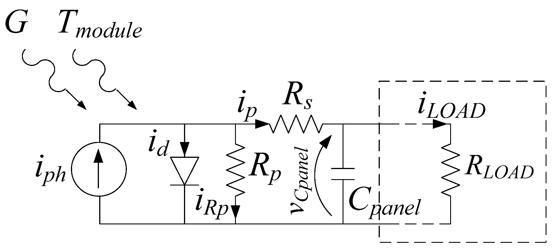
The basic equivalent circuit is shown in Figure 8. R_LOAD is a fictitious load connected to the PV array.

Performing simple calculations, Equation (21) becomes:

$$\begin{array}{l}\frac{d{v}_{C_{panel}}}{dt}=\left[-\frac{R_p+R_s+R_{LOAD}}{R_{LOAD}{C}_{panel}\left(R_p+R_s\right)}\right]v_{C_{panel}}+\\ +{\displaystyle [}\begin{array}{cc}\frac{1}{C_{panel}\left(1+\frac{R_s}{R_p}\right)}& -\frac{1}{C_{panel}\left(1+\frac{R_s}{R_p}\right)}\end{array}{\displaystyle ]}\left[\begin{array}{c}{i}_{ph}\\ i_d\end{array}\right]\end{array}$$

(22)

by assuming that:

$$x_p=v_{C_{panel}}u=\left[\begin{array}{c}{i}_{ph}\\ i_d\end{array}\right]$$

(23)

so that:

$$A_p=\left[-\frac{R_p+R_s+R_{LOAD}}{R_{LOAD}{C}_{panel}\left(R_p+R_s\right)}\right]B_p={\displaystyle [}\begin{array}{cc}\frac{1}{C_{panel}\left(1+\frac{R_s}{R_p}\right)}& -\frac{1}{C_{panel}\left(1+\frac{R_s}{R_p}\right)}\end{array}{\displaystyle ]}$$

(24)

and:

$$C_p=1D_p=0$$

(25)

Current i_ph is a function of irradiance G and of module temperature T_module as follows:

$$i_{ph}=\left[I_{sc}+K_t\left(T_{\mathrm{module}}-25\right)\right]\frac{G}{1000}$$

(26)

where K_t is the temperature coefficient:

$$K_t=\frac{NOCT-20}{800}$$

(27)

The normal operating cell temperature (NOCT) is usually reported in a PV module datasheet. Also the current i_d is a function of G and of T_module [26].

3.5. Transformers and Grid Model

The implementation of a detailed equivalent circuit for the LV-MV transformer as well as of a distributed parameters model for the AC grid is not feasible for computational effort reasons. Anyway, a satisfactory accuracy is obtained using a minimum order model as the one shown in Figure 5. Values of grid voltage sources, load resistors and load inductances are calculated referring to the primary side of the transformer.

3.6. PV Plant Model

Combination of models built for each component of the PV system in Figure 5 leads to a comprehensive state-space representation for the entire plant or for a specific subfield in the form of Equation (28). In this way, power and energy values at the power meter can be calculated from irradiance and cell temperature data by running such integrated state-space average model.

In this representation, an input is the RMS value of phase-to-phase grid voltage V_grid together with irradiance and module temperature. Alternatively, it can be assigned as a constant term into matrices. Control variables d and m are set by the control system described in Section 3.7.

Considering the whole PV system in Figure 5, its state-space representation is:

$$\{\begin{array}{l}\dot{x}=\overline{A}x+\overline{B}u\\ y=\overline{C}x+\overline{D}u\end{array}$$

(28)

where:

$$x=\left[\begin{array}{c}{v}_{C_{panel}}\\ i_{L_1}\\ v_{C_1}\\ x_1\\ \dots \\ \dots \\ x_{18}\end{array}\right]u=\left[\begin{array}{c}{i}_{ph}\\ i_d\\ V_{grid}\end{array}\right]y=x\mathrm{or}y=\left[\begin{array}{c}{x}_1\\ \dots \\ \dots \\ x_{12}\end{array}\right]$$

(29)

Matrix $\overline{A}$ is:

$$\overline{A}=A_{ON}d+A_{OFF}\left(1-d\right)$$

(30)

with:

$$A_{ON}=\left[\begin{array}{ccc}{A}_{O{N}_{1,1}}& \dots & A_{O{N}_{1,21}}\\ \dots & \dots & \dots \\ A_{O{N}_{21,1}}& \dots & A_{O{N}_{21,21}}\end{array}\right]A_{OFF}=\left[\begin{array}{ccc}{A}_{OF{F}_{1,1}}& \dots & A_{OF{F}_{1,21}}\\ \dots & \dots & \dots \\ A_{OF{F}_{21,1}}& \dots & A_{OF{F}_{21,21}}\end{array}\right]$$

(31)

Non-zero elements in matrix A_ON are listed here:

$$A_{O{N}_{1,1}}=-\frac{1}{C_{panel}\left(R_s+R_p\right)}{A}_{O{N}_{1,2}}=-\frac{1}{C_{panel}}{A}_{O{N}_{2,1}}=\frac{1}{L_1}{A}_{O{N}_{2,2}}=-\frac{r_{L_1}}{L_1}$$

(32)

$$A_{O{N}_{3,4}}=-\frac{\sqrt{3}m}{2C_1}\cos \left({\phi }_a-\frac{\pi }{6}\right)A_{O{N}_{3,5}}=\frac{\sqrt{3}m}{2C_1}\sin \left({\phi }_a-\frac{\pi }{6}\right)$$

(33)

$$A_{O{N}_{3,6}}=-\frac{\sqrt{3}m}{2C_1}\cos \left({\phi }_b-\frac{\pi }{6}\right)A_{O{N}_{3,7}}=\frac{\sqrt{3}m}{2C_1}\sin \left({\phi }_b-\frac{\pi }{6}\right)$$

(34)

$$A_{O{N}_{3,8}}=-\frac{\sqrt{3}m}{2C_1}\cos \left({\phi }_c-\frac{\pi }{6}\right)A_{O{N}_{3,9}}=\frac{\sqrt{3}m}{2C_1}\sin \left({\phi }_c-\frac{\pi }{6}\right)$$

(35)

$$A_{O{N}_{4,3}}=\frac{\sqrt{3}m}{12L_2}\cos \left({\phi }_a-\frac{\pi }{6}\right)A_{O{N}_{5,3}}=-\frac{\sqrt{3}m}{12L_2}\sin \left({\phi }_a-\frac{\pi }{6}\right)$$

(36)

$$A_{O{N}_{6,3}}=\frac{\sqrt{3}m}{12L_2}\cos \left({\phi }_b-\frac{\pi }{6}\right)A_{O{N}_{7,3}}=-\frac{\sqrt{3}m}{12L_2}\sin \left({\phi }_b-\frac{\pi }{6}\right)$$

(37)

$$A_{O{N}_{8,3}}=\frac{\sqrt{3}m}{12L_2}\cos \left({\phi }_c-\frac{\pi }{6}\right)A_{O{N}_{9,3}}=-\frac{\sqrt{3}m}{12L_2}\sin \left({\phi }_c-\frac{\pi }{6}\right)$$

(38)

and:

$$A_{O{N}_{4,4}}=A_{O{N}_{5,5}}=A_{O{N}_{6,6}}=A_{O{N}_{7,7}}=A_{O{N}_{8,8}}=A_{O{N}_{9,9}}=-\frac{r_{L_2}}{L_2}$$

(39)

$$A_{O{N}_{4,10}}=A_{O{N}_{5,11}}=A_{O{N}_{6,12}}=A_{O{N}_{7,13}}=A_{O{N}_{8,14}}=A_{O{N}_{9,15}}=-\frac{1}{3L_2}$$

(40)

$$A_{O{N}_{5,4}}=A_{O{N}_{7,6}}=A_{O{N}_{9,8}}=A_{O{N}_{11,10}}=A_{O{N}_{13,12}}=A_{O{N}_{15,14}}=A_{O{N}_{17,16}}=A_{O{N}_{19,18}}=A_{O{N}_{21,20}}=-\omega$$

(41)

$$A_{O{N}_{4,5}}=A_{O{N}_{6,7}}=A_{O{N}_{8,9}}=A_{O{N}_{10,11}}=A_{O{N}_{12,13}}=A_{O{N}_{14,15}}=A_{O{N}_{16,17}}=A_{O{N}_{18,19}}=A_{O{N}_{20,21}}=\omega$$

(42)

$$A_{O{N}_{10,4}}=A_{O{N}_{11,5}}=A_{O{N}_{12,6}}=A_{O{N}_{13,7}}=A_{O{N}_{14,8}}=A_{O{N}_{15,9}}=\frac{1}{C_2}$$

(43)

$$A_{O{N}_{10,16}}=A_{O{N}_{11,17}}=A_{O{N}_{12,18}}=A_{O{N}_{13,19}}=A_{O{N}_{14,20}}=A_{O{N}_{15,21}}=-\frac{1}{C_2}$$

(44)

$$A_{O{N}_{16,10}}=A_{O{N}_{17,11}}=A_{O{N}_{18,12}}=A_{O{N}_{19,13}}=A_{O{N}_{20,14}}=A_{O{N}_{21,15}}=\frac{1}{L_{LOAD}}$$

(45)

$$A_{O{N}_{16,16}}=A_{O{N}_{17,17}}=A_{O{N}_{18,18}}=A_{O{N}_{19,19}}=A_{O{N}_{20,20}}=A_{O{N}_{21,21}}=-\frac{R_{LOAD}}{L_{LOAD}}$$

(46)

The elements in A_OFF whose expression is different from the corresponding A_ON terms are:

$$A_{OF{F}_{1,2}}=A_{OF{F}_{2,1}}=0A_{OF{F}_{2,3}}=-\frac{1}{L_1}{A}_{OF{F}_{3,2}}=\frac{1}{C_1}$$

(47)

Matrix $\overline{B}$ is:

$$\overline{B}=B_{ON}d+B_{OFF}\left(1-d\right)$$

(48)

with:

$$B_{ON}=\left[\begin{array}{ccc}{B}_{O{N}_{1,1}}& B_{O{N}_{1,2}}& B_{O{N}_{1,3}}\\ \dots & \dots & \dots \\ B_{O{N}_{21,1}}& B_{O{N}_{21,2}}& B_{O{N}_{21,3}}\end{array}\right]B_{OFF}=B_{ON}$$

(49)

whose non-zero elements are:

$$B_{O{N}_{1,1}}=\frac{1}{C_{panel}\left(1+\frac{R_s}{R_p}\right)}{B}_{O{N}_{1,2}}=-\frac{1}{C_{panel}\left(1+\frac{R_s}{R_p}\right)}$$

(50)

$$B_{O{N}_{16,3}}=-\frac{\sqrt{2}}{L_{LOAD}}\cos \left({\phi }_{grida}\right)B_{O{N}_{17,3}}=\frac{\sqrt{2}}{L_{LOAD}}\sin \left({\phi }_{grida}\right)$$

(51)

$$B_{O{N}_{18,3}}=-\frac{\sqrt{2}}{L_{LOAD}}\cos \left({\phi }_{gridb}\right)B_{O{N}_{19,3}}=\frac{\sqrt{2}}{L_{LOAD}}\sin \left({\phi }_{gridb}\right)$$

(52)

$$B_{O{N}_{20,3}}=-\frac{\sqrt{2}}{L_{LOAD}}\cos \left({\phi }_{gridc}\right)B_{O{N}_{21,3}}=\frac{\sqrt{2}}{L_{LOAD}}\sin \left({\phi }_{gridc}\right)$$

(53)

Each state variable can be extracted as output of the system thanks to a proper assignment of matrix $\overline{C}$. Alternatively, the latter matrix is set as an identity matrix. Matrix $\overline{D}$ is null.

Evaluation of the energy produced by the plant is performed by building simple equations using variables from x₁ to x₁₂ i.e., by AC voltage and current components.

Values of DC and AC cables resistance, useful to calculate the distribution losses and to evaluate the same in case of different plant configurations, are added to resistive elements included in state-space matrices or inserted in the form of new resistive elements.

3.7. Control System

DC-DC converter stage is controlled in P&O MPPT mode. Control system of the grid connected inverter is implemented in qd reference frame using a common Phase Locked Loop (PLL) algorithm to regulate active and reactive power. Control subsystem for the d-axis current sets the DC-link voltage [28].

Time sampling of quantities in control system can be set larger than time step used for the simulation of PV plant e.g., 10x or more in order to allow a fast computational time. With reference to the specific case study discussed in this paper, design of control system needs to take into account additional constraints: maximum power internal threshold of each converter, power limitation strategy related to IGBT stack temperature and PPC limitation. The latter depends on thresholds fixed by the local utility company for the maximum power that the PV plant can deliver to the grid.

3.8. Parameters Identification

PV array parameters are identified exploiting data listed in the datasheet of modules and considering the power configuration of strings and stringboxes. On the contrary, some parameters e.g., R_s and R_p need to be identified. A suitable identification method, used for this work, is in [26]. Temperature coefficients of V_oc and I_sc reported in PV module datasheet and in Table 1 are also exploited.

About converters, detailed information on topology, hardware components and control system are usually not available due to know-how protection policies. It is worth noting that the modeling approach described in this paper allows to overcome this issue giving the opportunity to identify an equivalent behavioral model. To perform such identification, one of the many methods in literature for state-space functions can be used. In this work, identification process is performed using data collected by the monitoring system and applying a constrained minimums formulation focusing on the deviation between model outputs and real measurements [29]. Generally, let y_measured(k) be a given electrical variable measured by plant datalogger in the form of a timeseries having N time samples:

$$\left[Y_{measured}\right]=\left[\begin{array}{c}{y}_{measured}(1)\\ y_{measured}(2)\\ \dots \\ y_{measured}(k)\\ \dots \\ y_{measured}(N)\end{array}\right]$$

(54)

Corresponding quantity calculated by model is named y_model(k). Each y_model(k) sample can be expressed as the linear composition of parameters p_n and of terms h_ki. The latters fix the relation between y_model(k) and each p_i parameter for a given system input:

$$y_{\mathrm{mode}l}(k)=h_{k1}{p}_1+h_{k2}{p}_2+....+h_{kn}{p}_n$$

(55)

which is, for N time samples:

$$\left[\begin{array}{c}{y}_{\mathrm{model}}(1)\\ y_{\mathrm{model}}(2)\\ \dots \\ y_{\mathrm{model}}(k)\\ \dots \\ y_{\mathrm{model}}(N)\end{array}\right]=\left[\begin{array}{cccc}{h}_{11}& h_{12}& \dots & h_{1n}\\ h_{21}& h_{22}& \dots & h_{2n}\\ \dots & \dots & \dots & \dots \\ h_{k1}& h_{k2}& \dots & h_{kn}\\ \dots & \dots & \dots & \dots \\ h_{N1}& h_{N2}& \dots & h_{Nn}\end{array}\right]\left[\begin{array}{c}{p}_1\\ p_2\\ \dots \\ p_n\end{array}\right]$$

(56)

or:

$$\left[{\mathrm{Y}}_{\mathrm{model}}\right]=\left[H\right]\left[P\right]$$

(57)

Implementation of the constrained minimums formulation gives the optimal set of parameters reducing the deviation between measured values and the ones calculated by model:

$$\left[P\right]\cong {\left({\left[H\right]}^T\left[H\right]\right)}^{-1}{\left[H\right]}^T\left[Y_{measured}\right]$$

(58)

4. Model Validation

The MatLab/Simulink environment is the software platform for testing the introduced model. Proposed approach is compared to the detailed model in which high-frequency switching and related phenomena are included. Validation process involves both accuracy and complexity performances of the proposed model for different operating scenarios.

4.1. Model Running

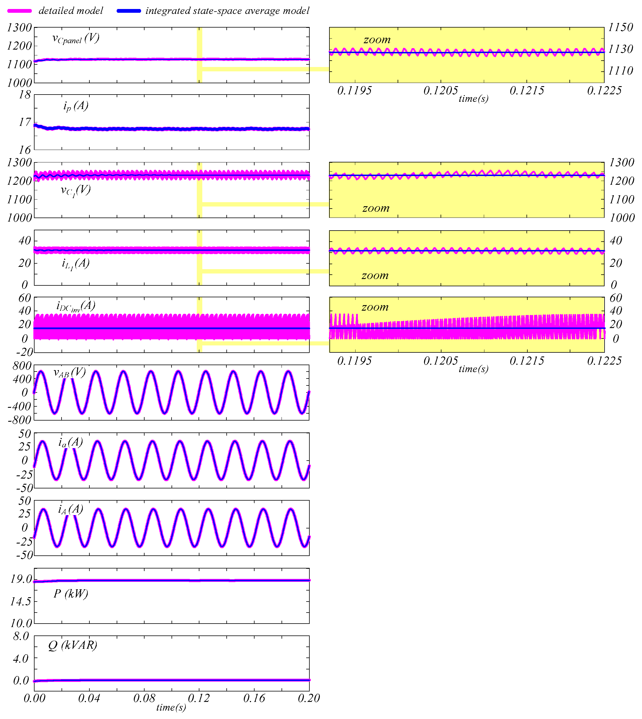
Figure 9 and Figure 10 show time plots of main electric quantities in a 18.9 kW PV subfield whose topology is the one shown in Figure 5. Referring to case study, this PV array is the basic generation unit to which a single MPPT in string inverters is applied. It is composed by two strings in parallel. Each string is the series connection of 30 PV modules, see datasheet in Table 1.

State-space average model is implemented in a straightforward way exploiting equations in Section 3.6 while in the detailed model all the components (PV modules, converters, filters, etc.) are placed into the simulation platform using their physical description. In Figure 9 and Figure 10 time plots obtained by the proposed model running in two operating scenarios are superimposed to the ones provided by detailed model in the same conditions.

Figure 9 depicts the waveforms of the main electric quantities obtained in case of 1000 W/m² as irradiance and of 25 °C as module temperature (standard test conditions, STC). Values of parameters for this simulation are in

Table 2. Parameters list for the simulation shown in Figure 9.

PV Module	See Table 1	Ts (s) *	1∙10−6
Ns	30	tend (s) *	0.2
Np	2	G(t0) (W/m2)	1000
Rs (Ω)	0.2 Ns/Np	Tmodule(t0) (°C)	25
Rp (Ω)	300 Ns/Np	fs,DCDC (kHz) **	10
Cpanel (µF)	110	fs,inv (kHz) ***	20
L1 (mH)	10	fn (Hz) ****	50
rL1 (Ω)	0.5	φa(t0) (rad)	2π/15
C1 (µF)	25	φgrida(t0) (rad)	0
L2 (mH)	34	VDCbus (V) *****	700
rL2 (Ω)	0.2	VgridLV (V)	400
C2 (µF)	0.22	VgridHV (kV)	34.5
RLOAD (Ω)	5	d(t0)	0.53
LLOAD (mH)	223	m(t0)	0.75

(*) T_s: simulation time step, t_end: simulation final time. (**) DC-DC converter switching frequency. (***) Inverter switching frequency. (****) Grid frequency. (*****) Rated DC-link voltage.

. The integrated state-space average model well matches the detailed model at both DC and AC side. Control system is able to force a null reactive power while active power at the power meter reaches about 18.5 kW i.e., close to the PV array STC rated power with a slight difference caused by power losses in DC and AC side.

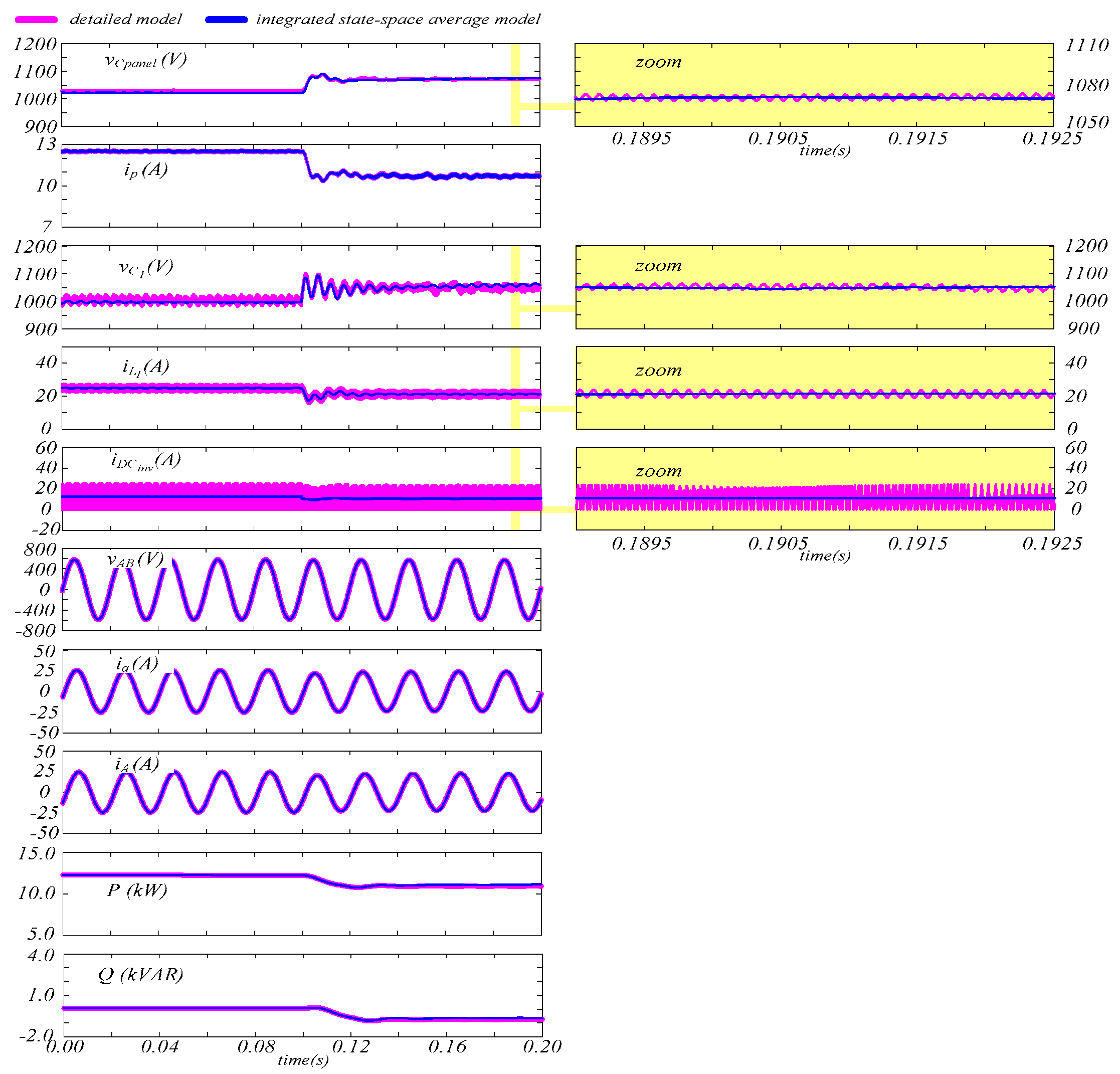
In Figure 10 irradiance is 800 W/m² and module temperature is 45 °C. Main parameters used in this simulation are listed in

Table 3. Parameters list for the simulation shown in Figure 10.

PV Module	See Table 1	Ts (s) *	1∙10−6
Ns	30	tend (s) *	0.2
Np	2	G(t0) (W/m2)	800
Rs (Ω)	0.2 Ns/Np	Tmodule(t0) (°C)	45
Rp (Ω)	300 Ns/Np	fs,DCDC (kHz) **	10
Cpanel (µF)	110	fs,inv (kHz) ***	20
L1 (mH)	10	fn (Hz) ****	50
rL1 (Ω)	0.5	φa(t0) (rad)	2π/23
C1 (µF)	25	φgrida(t0) (rad)	0
L2 (mH)	34	VDCbus (V) *****	700
rL2 (Ω)	0.2	VgridLV (V)	400
C2 (µF)	0.22	VgridHV (kV)	34.5
RLOAD (Ω)	5	d(t0)	0.5
LLOAD (mH)	223	m(t0)	0.75

(*) T_s: simulation time step, t_end: simulation final time. (**) DC-DC converter switching frequency. (***) Inverter switching frequency. (****) Grid frequency. (*****) Rated DC-link voltage.

. At time 0.1 s control system forces a non null reactive power requested by grid. Also in this case the average model is compliant to the detailed one.

Repeating similar comparisons for several scenarios, the average error caused by the proposed model with respect to the detailed one is always zero or very close to zero.

Finally, the integrated state-space average approach, built as described in previous sections, provides the average values of all the electric quantities in every operating condition. It can replace the detailed one in most analysis addressed to establish the performance of PV plants.

4.2. Execution Time Performance

Referring to the same PV system analyzed in the previous Section and shown in Figure 5, the advantages of the proposed approach have been evaluated in terms of execution time performance by implementing two different cases:

• Case A: the same simulation sample time is used for both the state-space average model and the detailed model. In such a case, the selected step size is 1∙10⁻⁶ s, established on the basis of dynamic features of the detailed model
• Case B: a larger simulation sample time (2∙10⁻⁵ s) is assigned to state-space average model since high-frequency switching and related phenomena are neglected. About the detailed model, its step size is the same of Case A otherwise it cannot run properly

For both A and B cases, four working scenarios have been simulated. To get a significant statistical database, each scenario has been executed 1000 times using two different processors named computer 1 and computer 2.

The evaluation of the execution time has been performed using some proper stopwatch functions in MatLab/Simulink environment. Relative difference in execution time is calculated by applying this equation:

$$\Delta t_{\%}=\frac{t_{issa}-t_{det}}{t_{det}}100$$

(59)

where, considering a given operating scenario, t_issa is the execution time of the integrated state-space average model while t_det is the execution time of the detailed model.

Table 4. Execution time performance evaluation, case A (simulation time step 1∙10⁻⁶ s), Computer 1 *.

	tdet	tissa	Δt%
Scenario 1	mean = 83.28 s std dev = 7.62 s	mean = 33.40 s std dev = 8.25 s	mean = −59.82% std dev = 8.92%
Scenario 2	mean = 83.01 s std dev = 8.41 s	mean = 31.01 s std dev = 6.46 s	mean = −62.35% std dev = 8.20%
Scenario 3	mean = 119.61 s std dev = 9.13 s	mean = 48.38 s std dev = 6.55 s	mean = −59.37% std dev = 7.79%
Scenario 4	mean = 149.57 s std dev = 8.79 s	mean = 58.79 s std dev = 5.66 s	mean = −60.64% std dev = 7.75%

* Computer 1, Hardware: Intel Core i3-4005U [email protected] GHz (4 CPUs), RAM 4096 MB, HD SSD 240 GB Read Speeds Up to 545 MB/s, 64 bit. 1000 simulations for each case. Charts Show Examples of Statistical Distribution. Simulation of the PV system described in Section 4.1, fixed time step is 1∙10⁻⁶ s. Scenario 1 and 2: simulation time 0.0 to 0.3 s. Scenario 3 and 4: simulation time 0.0 to 0.5 s. Scenario 1: 1000 W/m², 25 °C-Scenario 2: 800 W/m², 45 °C, non-zero reactive power is forced at 0.1 s-Scenario 3: irradiance increases from 800 W/m² to 950 W/m², module temperature increases from 40 °C to 55 °C-Scenario 4: irradiance decreases from 1000 W/m² to 850 W/m², module temperature decreases from 55 °C to 40 °C.

,

Table 5. Execution time performance evaluation, case A (simulation time step 1∙10⁻⁶ s), Computer 2 *.

	tdet	tissa	Δt%
Scenario 1	mean = 27.43 s std dev = 0.48 s	mean = 9.47 s std dev = 0.43 s	mean = −65.47% std dev = 1.67%
Scenario 2	mean = 27.38 s std dev = 0.37 s	mean = 9.04 s std dev = 0.54 s	mean = −66.96% std dev = 2.30%
Scenario 3	mean = 44.94 s std dev = 0.66 s	mean = 15.07 s std dev = 0.73 s	mean = −66.44% std dev = 1.97%
Scenario 4	mean = 40.04 s std dev = 0.52 s	mean = 14.86 s std dev = 0.72 s	mean = −62.86% std dev = 2.09%

* Computer 2, Hardware: Intel Core i7-8700K [email protected] GHz (12 CPUs), RAM 32768 MB, HD SSD 250 GB Read Speeds Up to 540 MB/s, 64 bit. 1000 simulations for each case. Simulation of the PV system described in Section 4.1, fixed time step is 1∙10⁻⁶ s. Scenario 1 and 2: simulation time 0.0 to 0.3 s. Scenario 3 and 4: simulation time 0.0 to 0.5 s. Scenario 1: 1000 W/m², 25 °C-Scenario 2: 800 W/m², 45 °C, non-zero reactive power is forced at 0.1 s-Scenario 3: irradiance increases from 800 W/m² to 950 W/m², module temperature increases from 40 °C to 55 °C-Scenario 4: irradiance decreases from 1000 W/m² to 850 W/m², module temperature decreases from 55 °C to 40 °C.

,

Table 6. Execution time performance evaluation, case B (simulation time step 2∙10⁻⁵ s), Computer 1 *.

	tdet	tissa	Δt%
Scenario 1	mean = 83.28 s std dev = 7.62 s	mean = 4.13 s std dev = 0.55 s	mean = −95.03% std dev = 0.62%
Scenario 2	mean = 83.01 s std dev = 8.41 s	mean = 3.20 s std dev = 0.25 s	mean = −96.12% std dev = 0.43%
Scenario 3	mean = 119.61 s std dev = 9.13 s	mean = 5.14 s std dev = 0.28 s	mean = −95.7% std dev = 0.41%
Scenario 4	mean = 149.57 s std dev = 8.79 s	mean = 6.40 s std dev = 0.35 s	mean = −95.8% std dev = 0.41%

* Computer 1, Hardware: Intel Core i3-4005U [email protected] GHz (4 CPUs), RAM 4096 MB, HD SSD 240 GB Read Speeds Up to 545 MB/s, 64 bit. 1000 simulations for each case. Simulation of the PV system described in Section 4.1, fixed time step is 2∙10⁻⁵ s. Scenario 1 and 2: simulation time 0.0 to 0.3 s. Scenario 3 and 4: simulation time 0.0 to 0.5 s. Scenario 1: 1000 W/m², 25 °C-Scenario 2: 800 W/m², 45 °C, non-zero reactive power is forced at 0.1 s-Scenario 3: irradiance increases from 800 W/m² to 950 W/m², module temperature increases from 40 °C to 55 °C-Scenario 4: irradiance decreases from 1000 W/m² to 850 W/m², module temperature decreases from 55 °C to 40 °C.

and

Table 7. Execution time performance evaluation, case B (simulation time step 2∙10⁻⁵ s), Computer 2 *.

	tdet	tissa	Δt%
Scenario 1	mean = 27.43 s std dev = 0.48 s	mean = 1.55 s std dev = 0.03 s	mean = −94.33% std dev = 0.15%
Scenario 2	mean = 27.38 s std dev = 0.37 s	mean = 1.56 s std dev = 0.01 s	mean = −94.31% std dev = 0.08%
Scenario 3	mean = 44.94 s std dev = 0.66 s	mean = 2.19 s std dev = 0.02 s	mean = −95.12% std dev = 0.09%
Scenario 4	mean = 40.04 s std dev = 0.52 s	mean = 1.65 s std dev = 0.02 s	mean = −95.88% std dev = 0.08%

* Computer 2, Hardware: Intel Core i7-8700K [email protected] GHz (12 CPUs), RAM 32768 MB, HD SSD 250 GB Read Speeds Up to 540 MB/s, 64 bit. 1000 simulations for each case. Simulation of the PV system described in Section 4.1, fixed time step is 2∙10⁻⁵ s. Scenario 1 and 2: simulation time 0.0 to 0.3 s. Scenario 3 and 4: simulation time 0.0 to 0.5 s. Scenario 1: 1000 W/m², 25 °C-Scenario 2: 800 W/m², 45 °C, non-zero reactive power is forced at 0.1 s-Scenario 3: irradiance increases from 800 W/m² to 950 W/m², module temperature increases from 40 °C to 55 °C-Scenario 4: irradiance decreases from 1000 W/m² to 850 W/m², module temperature decreases from 55 °C to 40 °C.

summarize the results in terms of execution time performance using a statistical approach based on mean value of Δt_% and on its standard deviation.

As expected, the novel behavioural model ensures a significant reduction in execution time for both the processors. In case A, the proposed model is about 3 times faster in comparison to the detailed model. In case B this difference rises to 25x.

4.3. Accuracy Evaluation

Evaluation of the accuracy of the proposed model is carried out by comparing power curves and daily energy with the measurements registered by power meters in the real plant.

Irradiance and module temperature timeseries, recorded by the monitoring system in the PV plant become inputs of the model together with the RMS value of the grid voltage.

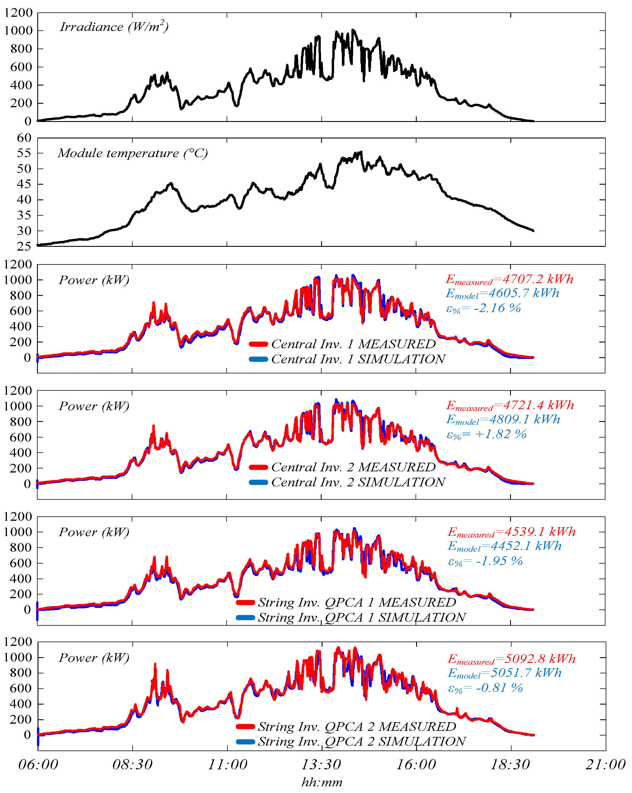
Figure 11 and Figure 12 show the PV plant operation during some days. Power curve of the model is superimposed to the measured one. During these days no unavailability, missing data or external constraints occur, so that comparison can be consistent.

For each day, the calculation of the percentage relative error for the daily energy is pointed out using this equation:

$${\epsilon }_{\%}=\frac{E_{model}-E_{measured}}{E_{measured}}100$$

(60)

In Figure 11, the maximum value of ε_% is registered for the bottom chart which refers to QPCA 2. In this case, the difference in daily energy between model and real data is 77.2 kWh corresponding to +2.32%. The minimum value of ε_%, −0.37%, is for QPCA 1 chart.

In Figure 12, the maximum value of ε_% is registered for central inverter 1. In this case, the difference in daily energy between model and real data is −101.5 kWh corresponding to −2.16%. The minimum value of ε_%, −0.81%, is for QPCA 2 chart.

Repeating similar analysis for all the days in the period from December 2017 to October 2019, it can be stated that maximum error caused by the model is in the range of 2.2–2.7% on a daily basis. This is an accuracy index for the model also for those cases in which the model is exploited to simulate plant behaviour in presence of missing data, PPC limitation, etc.

In case of partial shading as seen in the left picture of Figure 1, the consequent mismatch effects could worsen the ability of model to simulate the plant operation. Anyway, from a practical point of view, such effects can be usually neglected on the basis of the following points:

• Sampling time of quantities acquired by dataloggers in large PV plants is typically 1 min or more. This is a limit for the detection of fast variations of irradiance or temperature
• Very fast variations of irradiance or temperature (e.g., in the order of seconds) could perturb the acquired values but their effect is low. They also have limited effects on production because of the electrical and thermal capacity of the PV system. On the contrary, medium fast variations (in the order of minutes) create a fluctuation in the energy production while causing a variation in the model output which keeps very close to reality
• Since the proposed model has a full scalability, an alternative could be running the model for every string exploiting local irradiance data. Unfortunately, this requires the presence of thousands of irradiance sensors. Because of the high costs, in existing plants there are no more than three sensors per MW
• Evaluating the accuracy by applying Equation (60) for many days during which partial shading phenomena occur, the maximum error keeps around 2.5–2.7%

4.4. Sensitivity Analysis

With the purpose to evaluate the sensitivity of the model to parameters variation or uncertainty, the relative error ε_% calculated by using Equation (60) when identification is performed as shown in Section 3.8, is compared to ε_p% calculated with the same equation but considering two different cases:

• ε_p1.1%, in this case the value of a certain parameter is 1.1 times the optimal value identified by using Equation (58), optimal values are assigned to the other parameters
• ε_p0.9%, in this case the value of a certain parameter is 0.9 times the optimal value identified by using Equation (58), optimal values are assigned to the other parameters

Value of sensitivity for both cases is:

$$sen{s}_{1.1\%}={\displaystyle |}\left|{\epsilon }_{p1.1\%}\right|-\left|{\epsilon }_{\%}\right|{\displaystyle |}sen{s}_{0.9\%}={\displaystyle |}\left|{\epsilon }_{p0.9\%}\right|-\left|{\epsilon }_{\%}\right|{\displaystyle |}$$

(61)

Taking into account main parameters for every section of the PV plant and perturbing their basic values one by one as described above,

Table 8. Sensitivity in case of perturbation equal to 1.1 times the optimal parameter value.

Parameter	Sens1.1% (%)
Rs	1.32
Rp	1.10
Cpanel	0.88
L1	0.01
rL1	0.88
C1	0.01
L2	0.01
rL2	0.08
C2	0.16
RLOAD	0.01
LLOAD	0.01

and

Table 9. Sensitivity in case of perturbation equal to 0.9 times the optimal parameter value.

Parameter	Sens1.1% (%)
Rs	1.28
Rp	1.15
Cpanel	0.98
L1	0.01
rL1	0.88
C1	0.02
L2	0.02
rL2	0.11
C2	0.16
RLOAD	0.01
LLOAD	0.01

report the average results obtained by running the model for several days in the period from December 2017 to October 2019.

As expected, it emerges that parameters belonging to PV array model have a large sensitivity causing the worsening of accuracy in case of deviation from optimal values. The same is for r_L1. The other parameters feature a low sensitivity.

5. Performance Comparison between Central and String Inverters

5.1. Relevance of the Introduced Model in Supporting Data Analysis

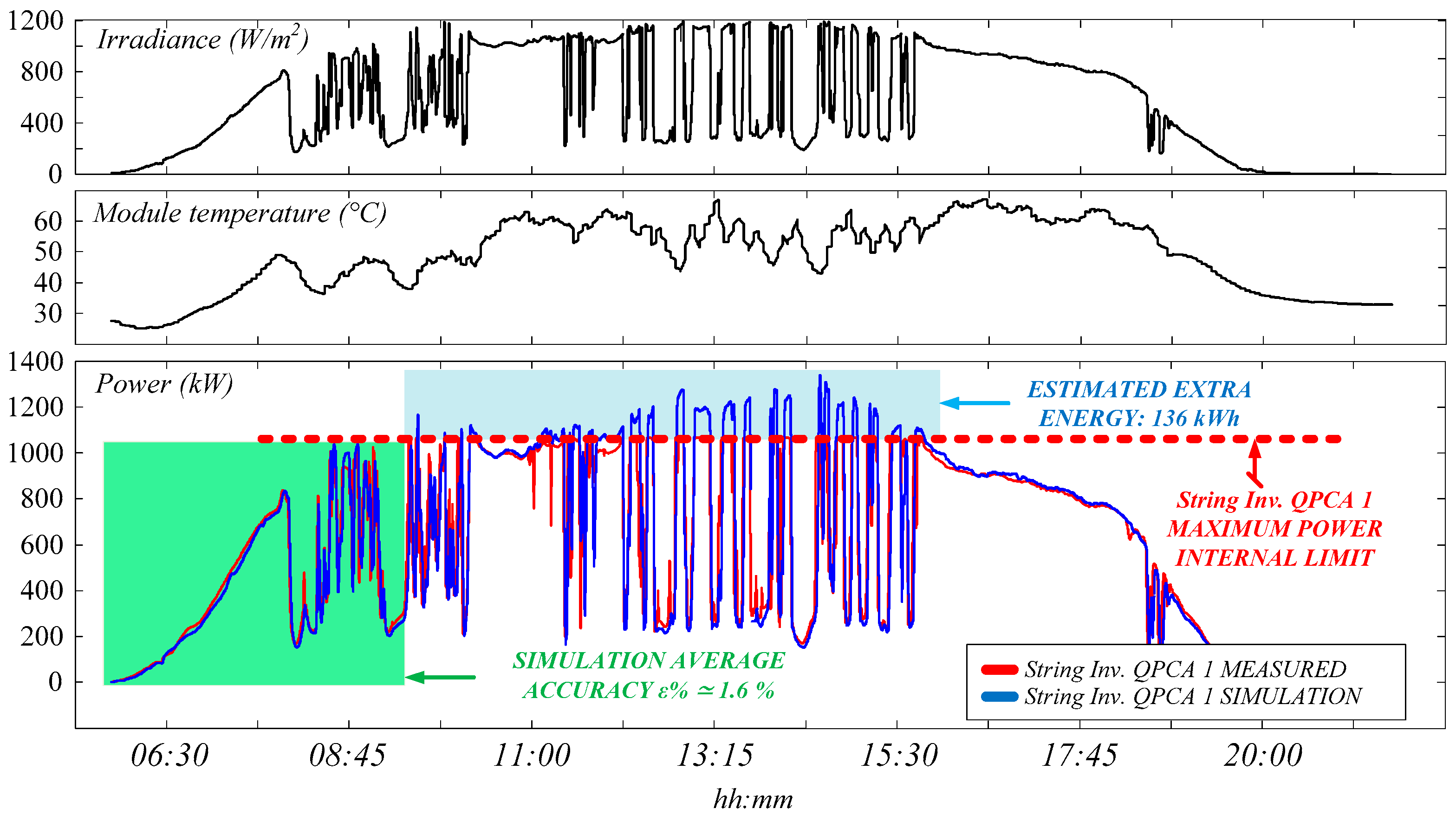
Referring to the case study, the usefulness of the proposed modeling approach is highlighted in this Section by showing some examples. In Figure 13 the power measured at the meter of the string inverters group QPCA 1 is compared to the power curve obtained in simulation for the same subfield (whose rated DC power is 1209.6 kW) in a day during which a power limitation occurs because of the inverter internal maximum power threshold. Power plots indicate that, thanks to the model simulation, theoretical extra-energy is estimated with a good accuracy.

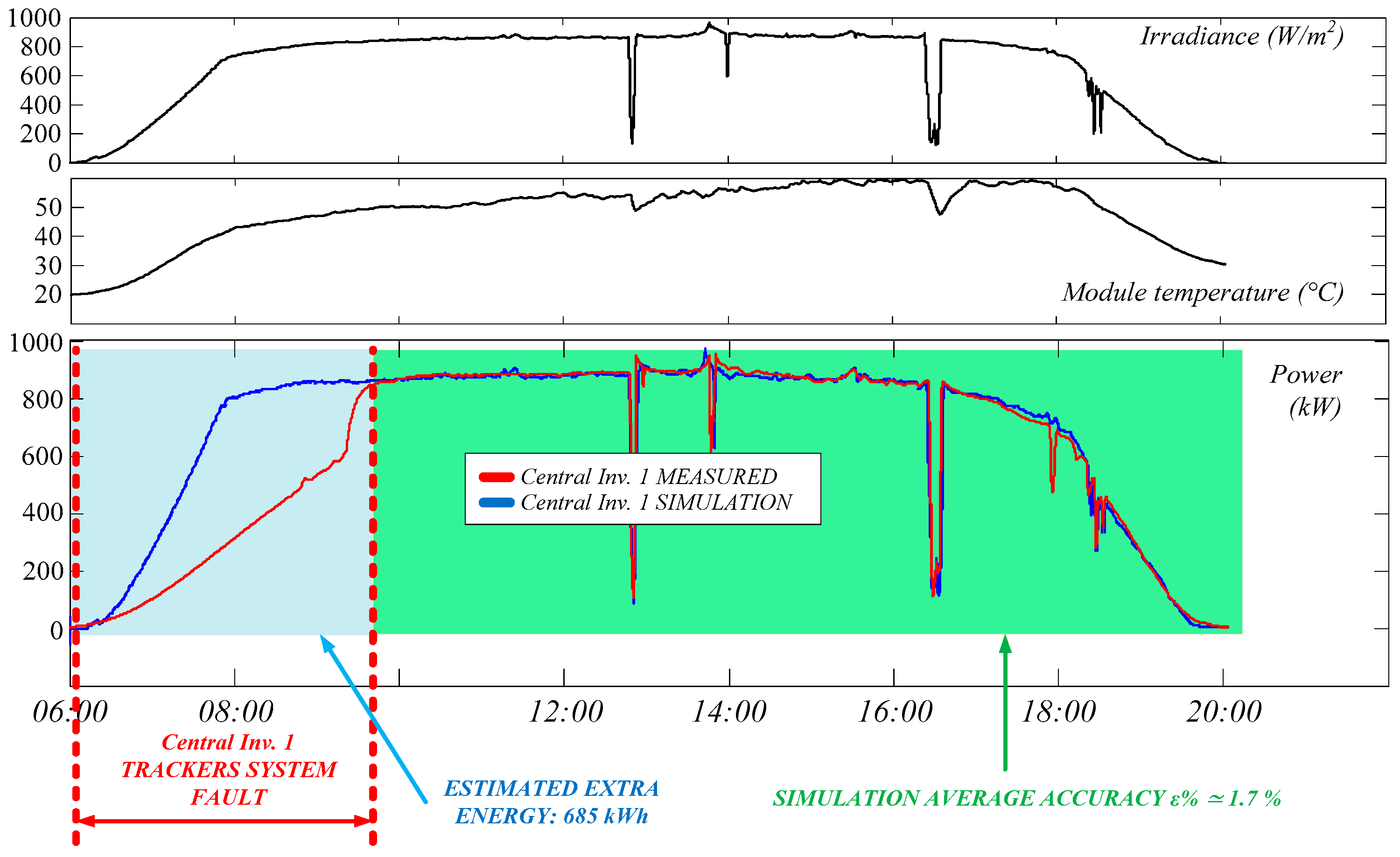
In Figure 14 model is applied to estimate the energy lost in central inverter 1 subfield caused by a fault in solar trackers power supply. Also in this case, the model is able to overcome wrong data due to the abnormal operation.

These examples highlight how the introduced model is a very useful tool to track the behaviour of PV plant in normal operation as well as in case of missing data, PPC limitation due to grid capability and so on.

5.2. Central vs. String Inverters: Comparison Results

Performances of central and string inverters in case study have been compared looking at the post-commissioning period (5 months long) from December 2017 to April 2018 i.e., during summer and autumn in Brazil. Basic equation used to evaluate the gain obtained by string converters G_{string_inv} is:

$$G_{string\_inv}=\frac{\frac{E_{string\_inv}}{P_{string\_inv}}-\frac{E_{central\_inv}}{P_{central\_inv}}}{\frac{E_{central\_inv}}{P_{central\_inv}}}100$$

(62)

where, on a daily basis, E_{string_inv} is the energy produced by string inverters (or by a QPCA), E_{central_inv} is the energy produced by central inverters (or by a single central inverter), P is the DC rated power of each subfield. Such comparison criterion corresponds to the comparison between performance ratio values.

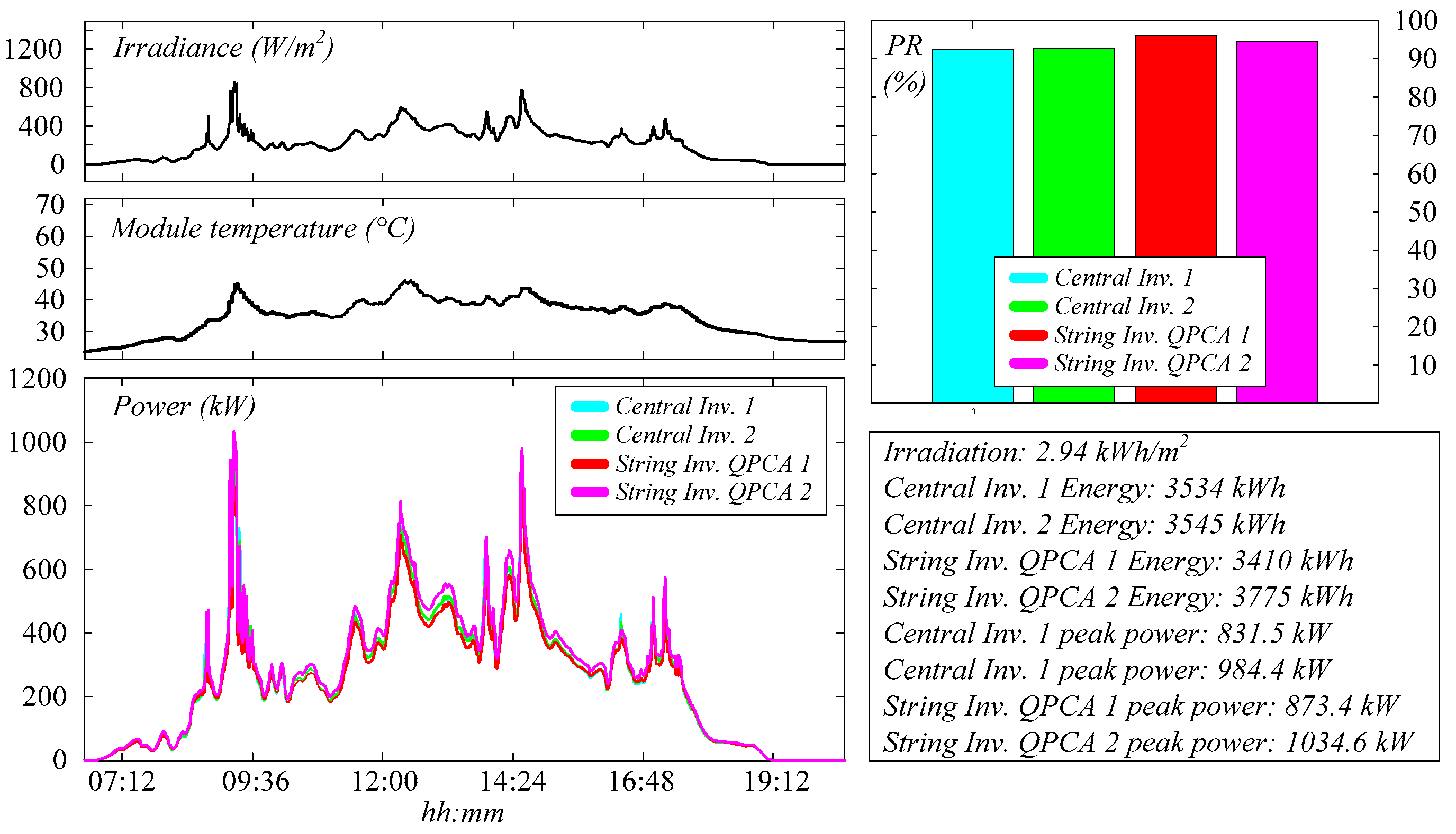
Figure 15 shows the energy produced in subfields with central and string inverters measured during a cloudy day, in absence of power derating, unavailability, PPC limitation or other constraints. In this specific case, the gain of string inverters subfield in comparison to central inverters is +1.5%, calculated by Equation (62).

This calculation has been repeated for all the days in the considered period. In case of issues caused by wrong data, PPC limitation, partial unavailability, etc. occurring for one or more converters, model presented in this paper has been used to replace data coming from the real PV plant as shown in the previous Section.

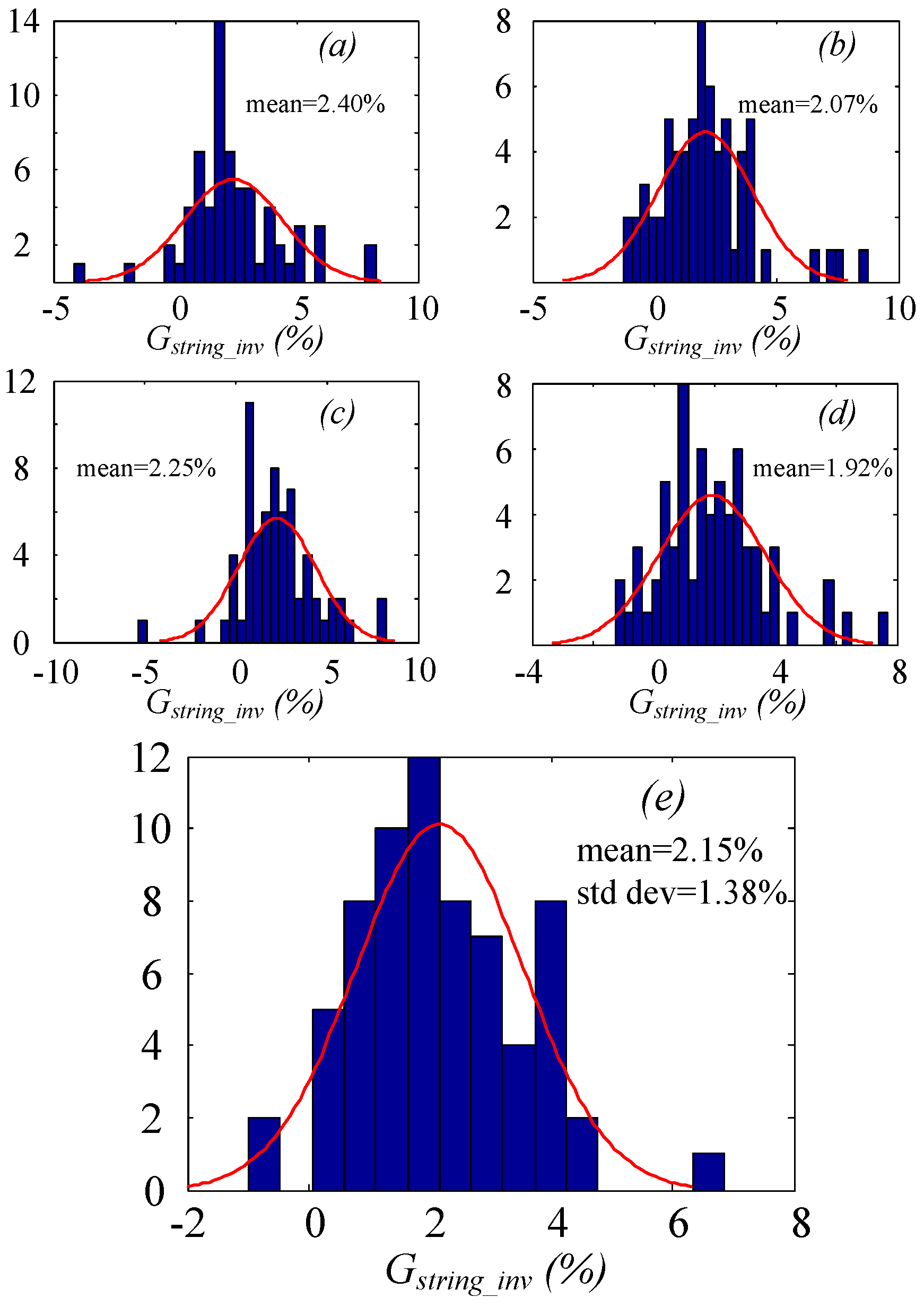
Referring to the fixed time period, aggregated results are reported in Figure 16 with distribution charts including a normal density function fitting curve. Finally, the average gain obtained by the string converters is around +2.1% in terms of daily production, with a standard deviation of about 1.3%.

6. Conclusions

This work deals with behavioral modeling of large PV plants. To evaluate the performance of distributed multi-stage converters in presence of issues caused by erroneous data, unavailability or external constraints, a new integrated state-space average model addressed to large or utility-scale PV plants has been introduced getting a satisfactory tradeoff between computational effort and simulation accuracy. A straightforward way for the calculation of the average DC-link current from the direct-sequence components of AC currents has been developed and exploited to reduce the computational complexity without decreasing the accuracy level.

Based on the calculation of the daily energy production in the period from December 2017 to October 2019, the maximum error caused by the model is in the range of 2.2–2.7% with respect to the energy measured by power analyzers. A case study has been investigated focusing on performance comparison between central and string converters installed for testing purpose in two subfields of a 300 MW PV plant in Brazil. Elaboration of data acquired by the monitoring system for 5 months in the PV plant is effectively supported by the developed model. Aggregate results highlight that string inverters ensure a gain of about 2% in terms of produced energy.

Future works will be addressed to the identification of phenomena leading to mismatch effects compensated by string inverters. Moreover, the same modeling approach will be applied for other real PV plants with distributed converters having different size and power configuration.

References

- Strache, S.; Wunderlich, R.; Heinen, S. A Comprehensive, Quantitative Comparison of Inverter Architectures for Various PV Systems, PV Cells, and Irradiance Profiles. IEEE Trans. Sustain. Energy 2014, 5, 813–822. [Google Scholar] [CrossRef]
- Birane, M.; Larbes, C.; Checknane, A. A comparative study and performance evaluation of central and distributed topologies of photovoltaic system. Int. J. Hydrogen Energy 2017, 42, 8703–8711. [Google Scholar] [CrossRef]
- Zeb, K.; Uddin, W.; Khan, M.A.; Ali, Z.; Ali, M.U.; Christofides, N.; Kim, H.J. A comprehensive review on inverter topologies and control strategies for grid connected photovoltaic system. Renew. Sustain. Energy Rev. 2018, 94, 1120–1141. [Google Scholar] [CrossRef]
- Harb, S.; Kedia, M.; Zhang, H.; Balog, R.S. Microinverter and string inverter grid-connected photovoltaic system—A comprehensive study. In Proceedings of the 39th Photovoltaic Specialists Conference PVSC, Tampa, FL, USA, 16–21 June 2013. [Google Scholar]
- Obi, M.; Bass, R. Trends and challenges of grid-connected photovoltaic systems—A review. Renew. Sustain. Energy Rev. 2016, 58, 1082–1094. [Google Scholar] [CrossRef]
- Dolara, A.; Leva, S.; Manzolini, G. Comparison of different physical models for PV power output prediction. Sol. Energy 2015, 119, 83–99. [Google Scholar] [CrossRef] [Green Version]
- Cuce, E.; Cuce, P.M.; Karakas, I.H.; Bali, T. An accurate model for photovoltaic (PV) modules to determine electrical characteristics and thermodynamic performance parameters. Energy Convers. Manag. 2017, 146, 205–216. [Google Scholar] [CrossRef]
- Barth, N.; Jovanovic, R.; Ahzi, S.; Khaleel, M.A. PV panel single and double diode models: Optimization of the parameters and temperature dependence. Sol. Energy Mater. Sol. Cells 2016, 148, 87–98. [Google Scholar] [CrossRef]
- Duran, E.; Galan, J.; Andujar, J.M.; Sidrach-de-Cardona, M. A new method to obtain I–V characteristics curves of photovoltaic modules based on SEPIC and Cuk converters. EPE J. 2008, 18, 5–15. [Google Scholar] [CrossRef]
- Pereira, H.A.; Freijedo, F.D.; Silva, M.M.; Mendes, V.F.; Teodorescu, R. Harmonic current prediction by impedance modeling of grid-tie inverters: A 1.4 MW PV plant case study. Electr. Power Energy Syst. 2017, 93, 30–38. [Google Scholar] [CrossRef]
- Trujillo, C.L.; Santamaria, F.; Gaona, E.E. Modeling and testing of two-stage grid-connected photovoltaic micro-inverters. Renew. Energy 2016, 99, 533–542. [Google Scholar] [CrossRef]
- Trejos, A.; Gonzales, D.; Ramon-Paja, C.A. Modeling of Step-up grid-connected photovoltaic system for control purposes. Energies 2012, 5, 1900–1926. [Google Scholar] [CrossRef]
- Fujii, K.; Noto, Y.; Okuma, Y. 1-MW solar power inverter with boost converter using all SiC power module. EPE J. 2016, 26, 165–173. [Google Scholar] [CrossRef]
- Guerrero-Perez, J.; De Jodar, E.; Gomez-Lazaro, E.; Molina-Garcia, A. behavioural modeling of grid-connected photovoltaic inverters: Development and assessment. Renew. Energy 2014, 68, 686–696. [Google Scholar] [CrossRef]
- Li, Y.; Chen, X.M.; Zhao, B.Y.G.; Zhao, Z.G.; Wang, R.Z. Development of a PV performance model for power output simulation at minutely resolution. Renew. Energy 2017, 111, 732–739. [Google Scholar] [CrossRef]
- Ayad, A.; Kennel, R. A comparison of quasi-Z-source inverter and conventional two-stage inverters for PV applications. EPE J. 2017, 27, 45–59. [Google Scholar] [CrossRef]
- Almeida, M.P.; Munoz, M.; de La Parra, I.; Perpinian, O. Comparative study on PV power forecast using parametric and nonparametric PV models. Sol. Energy 2017, 155, 854–866. [Google Scholar] [CrossRef] [Green Version]
- Tan, R.H.G.; Hoo, L.Y.H. DC-DC converter modeling and simulation using state-space approach. In Proceedings of the IEEE Conference on Energy Conversion CENCON, Johor Bahru, Malaysia, 19–20 October 2015. [Google Scholar]
- Chiniforoosh, S.; Jatskevich, J.; Yazdani, A.; Sood, V.; Dinavahi, V.; Martinez, J.A.; Ramirez, A. definitions and applications of dynamic average models for analysis of power systems. IEEE Trans. Power Deliv. 2010, 25, 2655–2669. [Google Scholar] [CrossRef]
- Kanimozhi, G.; Meenakshi, J.; Sreedevi, V. Small signal modeling of a DC-DC type double boost converter integrated with SEPIC converter using state space averaging approach. Energy Procedia 2017, 117, 835–846. [Google Scholar] [CrossRef]
- Liu, X.; Cramer, A.M. Three-phase inverter modeling using multifrequency averaging with third harmonic injection. In Proceedings of the IEEE Energy Conversion Congress and Exposition ECCE, Milwaukee, WI, USA, 18–22 September 2016. [Google Scholar]
- Coronado-Mendoza, A.; Perez-Cisneros, M.A.; Dominguez-Navarro, J.A.; Osuna-Enciso, V.; Zuniga-Grajeda, V.; Gurubel-Tun, K.J. Dynamic phasors modeling for a single phase two stage inverter. Electr. Power Syst. Res. 2016, 140, 854–865. [Google Scholar] [CrossRef]
- Lin, Z.; Ma, H. Modeling and analysis of three-phase inverter based on generalized state space averaging method. In Proceedings of the 39th Annual Conference of the IEEE Industrial Electronic Society IECON, Vienna, Austria, 10–13 November 2013. [Google Scholar]
- Kolar, J.W.; Round, S.D. Analytical calculation of the RMS current stress on the DC-link capacitor of voltage-PWM converter systems. IEE Proc. Electr. Power Appl. 2006, 153, 535–543. [Google Scholar] [CrossRef] [Green Version]
- Pei, X.; Zhou, W.; Kang, Y. Analysis and calculation of DC-Link current and voltage ripples for three-phase inverter with unbalanced load. IEEE Trans. Power Electron. 2015, 30, 5401–5412. [Google Scholar] [CrossRef]
- Villalva, M.G.; Gazoli, J.R.; Filho, E.R. Comprehensive approach to modeling and simulation of photovoltaic arrays. IEEE Trans. Power Electron. 2009, 24, 1198–1208. [Google Scholar] [CrossRef]
- Kerekes, T.; Koutroulis, E.; Sera, D.; Teodorescu, R.; Katsanevakis, M. An optimal method for designing large PV plants. IEEE J. Photovolt. 2013, 3, 814–822. [Google Scholar] [CrossRef]
- Ali, Z.; Christofides, N.; Hadjidemetriou, L.; Kyriakides, E.; Yang, Y.; Blaabjerg, F. Three-phase phase-locked loop synchronization algorithms for grid-connected renewable energy systems: A review. Renew. Sustain. Energy Rev. 2018, 90, 434–452. [Google Scholar] [CrossRef] [Green Version]
- Nobile, G.; Cacciato, M.; Scarcella, G.; Scelba, G.; Vasta, E.; Di Stefano, A.G.F.; Leotta, G.; Pugliatti, P.M.; Bizzarri, F. Distributed converters in large PV plants: Performance analysis supported by behavioral models. In ELECTRIMACS 2019; Lecture Notes in Electrical Engineering; Zamboni, W., Petrone, G., Eds.; Springer: Cham, Switzerland, 2020; Volume 604, pp. 553–566. [Google Scholar]
Figure 1.
Pictures of the 300 MW PV plant in Brazil.
Figure 2.
Scheme of the 2.5 MW subfield with central inverters.
Figure 3.
Scheme of the 2.5 MW subfield with string inverters.
Figure 4.
PV plant basic scheme. G is the measured irradiance, Tmodule is the module temperature, P&O is the Perturb and Observe algorithm.
Figure 5.
Block diagram of a PV system with multi-stage conversion system.
Figure 6.
DC-DC converter basic topology and its state-space form including duty cycle variation.
Figure 7.
Grid connected inverter and AC filtering stage, basic topology.
Figure 8.
Simplified equivalent circuit used to build the basic state-space representation of the PV array.
Figure 9.
Simulation of a 18.9 kW PV subfield (2 strings in parallel, each string is composed by the series connection of 30 315 W PV modules). PV system topology is represented in
Figure 5, technical data of components are listed in