Self-Reinforcing Electricity Price Dynamics under the Variable Market Premium Scheme


Department of Energy Systems Analysis, Institute of Engineering Thermodynamics, German Aerospace Center, Curiestrasse 4, 70563 Stuttgart, Germany
*
Author to whom correspondence should be addressed.
†
All authors contributed equally.
‡
Current affiliation: Wattsight AS, 4841 Arendal, Norway.
Energies 2020, 13(20), 5350; https://0-doi-org.brum.beds.ac.uk/10.3390/en13205350
Submission received: 31 July 2020
/
Revised: 6 October 2020
/
Accepted: 9 October 2020
/
Published: 14 October 2020
(This article belongs to the Special Issue Uncertainties and Risk Management in Competitive Energy Markets)
Abstract
:We report a potential self-reinforcing design flaw in the variable market premium scheme that occurs if variable renewable energy power plants receiving a premium become price-setting in the market. A high share of renewable energy is a goal of many countries on their transformation path to a sustainable future. Accordingly, policies like feed-in tariffs have been in place for many years in many countries to support investment. To foster market alignment, variable market premia have been introduced in at least 12 European countries and a further dozen additional countries world-wide. We demonstrate both with a mathematical model and different scenarios of an agent-based simulation that the combination of variable premia and a high share of hours in which renewables are price-setting may lead to a self-reinforcing downward spiral of prices if unchecked. This is caused by the market premium opening up the bidding space towards negative prices. We discuss possible objections and countermeasures and evaluate the severity of this market design flaw.
1. Introduction
Variable renewable energies (VREs) have come a long way from exotic newcomers to essential building blocks of the energy systems of today. Currently, large industrialized countries in the EU, e.g., Germany and Denmark, have VRE-shares of more than 40% [1,2,3]. In addition, it has been convincingly demonstrated that energy systems with VRE shares of 80–100% are feasible [4,5,6].
Many support and deployment policies have been in place for decades in many countries in order to facilitate this transition to cleaner energy. The central goal of these policies is usually to ensure refinancing of power plants generating electricity from renewable energy sources. Often, in their introductory phase, fixed feed-in tariffs have been successfully promoting renewables by significantly reducing investment risks. With fixed feed-in tariffs, renewable energy plant owners receive a fixed remuneration for each kWh of electricity fed into the grid. They have a proven track record enabling new renewable technologies to enter the market [7].
However, since the beginning of integrating renewables into energy systems, a major transition has taken place, since the goal now is to move towards a new market design by creating liberalized and competitive electricity markets in the EU. Accordingly, a large number of various support schemes has been introduced to support this transition [8]. Our article is concerned about a potential design flaw of variable market premia. This flaw could affect electricity prices and market premia even before expansion targets are reached.
In order to place our analysis in context it is helpful to take a look at the different support schemes that exist. For supply-oriented support schemes a general distinction can be made between price-based and volume-based support instruments [9]. Schemes are often characterized by effectiveness, efficiency, impact and feasibility [10]. Each scheme is designed to achieve specific subgoals [7] and comes with its own advantages and disadvantages. Price-based schemes set financial incentives. The resulting volume is not determined and may vary. In contrast, volume-based schemes require a fixed volume resulting in variable prices. For price-based schemes, costs cannot be predicted beforehand [9]. Volume-driven schemes, in contrast, are quite inflexible. If, for example, the targeted volume is exhausted quickly, further expansion is difficult and requires setting up a new scheme. Typical instruments of price-based schemes include feed-in tariffs, market premia, contracts for difference (CFD, also referred to as symmetrical market premium or double-sided sliding premium) or investment support, low interest loans and tax exemptions. Volume-based schemes include instruments like quota obligations, tender or auction-schemes [9].
In the last few years, market premia were introduced as a widespread approach to align supply and demand, since fixed feed-in tariffs are very well suited to ensure refinancing but do not set any incentives for demand orientation. Policy instruments with market premia are one of the major pillars of European VRE market integration legislation: According to RES LEGAL, at least the 12 European countries currently employ some form of variable market premium scheme (Croatia, Czech Republic, Denmark, Finland, France, Germany, Greece, Italy, Lithuania, Luxemburg, the Netherlands and the United Kingdom; see [11]). Moreover, some current VRE auction designs rely on a variable market premium, for example in Denmark, Germany, Italy and the Netherlands. Additionally, more than a dozen of countries world-wide also employ feed-in tariffs with premium payments [12].
In particular, market premia are designed to eliminate the risks of renewable power plant operators [13,14]. They come in two flavors: either as fixed or as variable (sliding or floating) premium. Both variants are designed to increase demand-oriented feed-in and decentralized direct marketing [9]. By dynamically adjusting the variable premium to a target strike price, the total gain for the plant operator remains constant even for low electricity market prices to ensure refinancing. Another design option is the symmetrical market premium, also referred to as double-sided sliding premium or contracts for difference. In this case the technologies receive a contract, which tops up the income per MWh from the average market price to a target strike price stated in the contract. If market prices exceed the target price the contract decreases the electricity market revenues to the strike price level [15,16].
In this study, we focus on the design of the variable premium as computed as the ex-post difference between the energy-source-specific market value (usually averaged over an accounting period of e.g., 1 month) and a predefined energy-source-specific reference tariff level. Latter is usually calculated in accordance with the energy- source-specific levelized cost of electricity (LCOE) [17] to ensure refinancing.
However, this type of premium has been introduced for markets with low shares of VRE [18]. Given that current transition goals involve very high shares of VRE, this article analyzes a design problem with both a variable market premium and high shares of VRE leading to self-reinforcing downward electricity price dynamics and increasing premia. High premia may jeopardize political acceptance of VRE and highly negative prices indicate an overproduction, which actually does not happen. These effects might counteract an effective and efficient further integration of renewables. We also list solutions in the discussion.
The rest of the article is structured as follows. We first present a mathematical model that is reduced to the mathematical bare-bones of the flaw and which shows that the problem of falling market prices and increasing premia is inherent to its structure. In the Results, we substantiate our claims with model results from an agent-based simulation, to demonstrate that this effect also arises under more complex and realistic conditions. Finally, in the Discussion, we raise possible objections concerning simulation assumptions, technological influences and current regulations. Possible solutions are also discussed.
2. Methods
We employed two different methods to show the self-reinforcing dynamics of variable market premia. First, a plain mathematical model was used to illustrate the dynamics under idealized assumptions. Second, we applied a tried and tested, full-blown agent-based energy market simulation tool with scenarios of different complexity. Taken together, both methods were able to establish that this self-reinforcing mechanism would arise in any case if just a few conditions were met (mathematical model) and also if the market situation was more realistic (especially the extended scenario). To further explore sensitivities of our modeling, we present results of additional scenarios in Appendix A (Appendix A.2 and Appendix A.3).
2.1. Plain Mathematical Model
Consider a simplified electricity market with uniform pricing and two power plant technologies without start-up or ramping constraints serving a fixed demand. Suppose there is one power plant technology I with marginal production cost of , and a new technology N with marginal production cost . Here, the term “marginal cost” represents the cost of producing one more unit of electric energy. Both capacities of I and N are dispatchable. Together, they are always able to cover the demand. After each accounting period , technology N receives an ex-post variable premium to recover its LCOE , i.e.,
with referring to the technology specific market value for electricity in the accounting period. LCOE represent the average cost of electricity generation over the lifetime of the power plant. For power plants with high investment cost but no fuel cost, e.g., VRE technologies, marginal cost are typically much lower than LCOE.
In a competitive energy-only market, generators would offer their capacity at marginal production costs [19,20]. In our model, this condition holds true for technology I which offers at price . In contrast, technology N is willing to offer at a price equal to its marginal cost minus the variable market premium it is expecting to receive in this accounting period. This bidding strategy would be revenue-neutral if technology N was price-setting. Since the market premium is paid ex-post, an estimate of the premium for the current accounting period is required. Therefore, it is assumed that the market premium for the current accounting period is estimated using its value from the previous accounting period, i.e., . This assumption does not affect the results in a major way, as we will argue in the Discussion (Objection A).
2.2. Agent-Based Simulation
For the simulation-based analyses we used the model AMIRIS (Agent-based Market model for the Investigation of Renewable and Integrated energy Systems) [21,22,23,24], an agent-based wholesale electricity market model for Germany. The model allows studying the impact of energy policy instruments on the economic performance of power plant operators and marketers. The model had an hourly resolution and computed wholesale electricity prices endogenously based on the simulation of strategic bidding behavior of prototyped market actors. This bidding behavior did not only reflect marginal prices, but it also considered effects of support instruments like market premia. Hence, AMIRIS focused on the perspective of the actors within the energy system, their interactions and competition. Uncertainties of the actors (e.g., amount of the market premium or feed-in of renewables) could be explicitly considered and reflected in the strategies. Each agent may have had its own goal and could be defined with its own decision-making rules. Traders, for example tried to maximize their profits. Other agents provided functions to the simulations—e.g., the energy market clearing was provided by an energy exchange agent. In this way, the energy system could be simulated component by component and actor by actor [25]. AMIRIS did not have a higher-level objective function. Instead, the simulation results were generated from the interplay of the actions of the individual actors depicted as agents under selected regulatory conditions. Further information and a model scheme are provided in Appendix A.1 and in [21,22,23,24].
In AMIRIS, the modelled electricity sub-markets were calibrated and validated with a fundamental approach for the merit-order model using empirical data in the classical sense. The day-ahead spot market model was validated for different years (2008, 2012–2016) in order to be able to make robust statements about electricity price developments [25,26].
Two scenarios were developed for this study: the first, simple scenario consists of only two electricity generation technologies, photovoltaic (PV, 200 GW) and gas (120 GW) and a carbon price of 0 €/t. In this case, gas power plants produced at a fixed marginal cost of 47.13 €/MWh. The aim of this simple scenario was to illustrate the principal mechanism of the effect discovered. A second scenario included more technologies: PV (200 GW), wind onshore (80 GW), wind offshore (20 GW), different conventional generation technologies (together 80 GW) with varying marginal costs and 20 GW of storage technologies. The carbon price was set at 50 €/t. The objective of this scenario was to check whether the discovered effect also held in a more complex and realistic environment.
The simulations were each conducted for 1 year with load and PV as well as wind profiles from the Open Power System Data [27].
3. Results
3.1. Results from Plain Mathematical Modeling
We distinguish between three cases.
3.1.1. Case 1: No Market Impact
Suppose that the marginal costs are and and the levelized cost of N is . Thus, expecting a non-negative premium, the merit order holds true. We further assume that technology N cannot cover the entirety of the demand at any time. Therefore, technology I sets the price and the market value of technology N equals . Hence, following Equation (1) the premium (difference between cost and price) is paid to N to recover its costs. In the depicted case, market prices, market values and premia do not change over time. The policy instrument works as intended to ensure refinancing while not distorting market prices.
3.1.2. Case 2: Moderate Market Influence
Now suppose that technology N can cover the entirety of the demand for a constant fraction of each accounting period. In this case, technology N would set the market price at these times to . At the other times, i.e., with a share of , the market price would remain at as set by technology I. As a result, the market value of the accounting periods is defined by
Inserting Equation (1) into Equation (2) and assuming as explained above yields
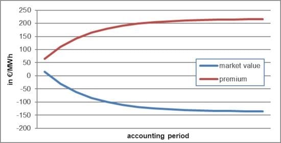
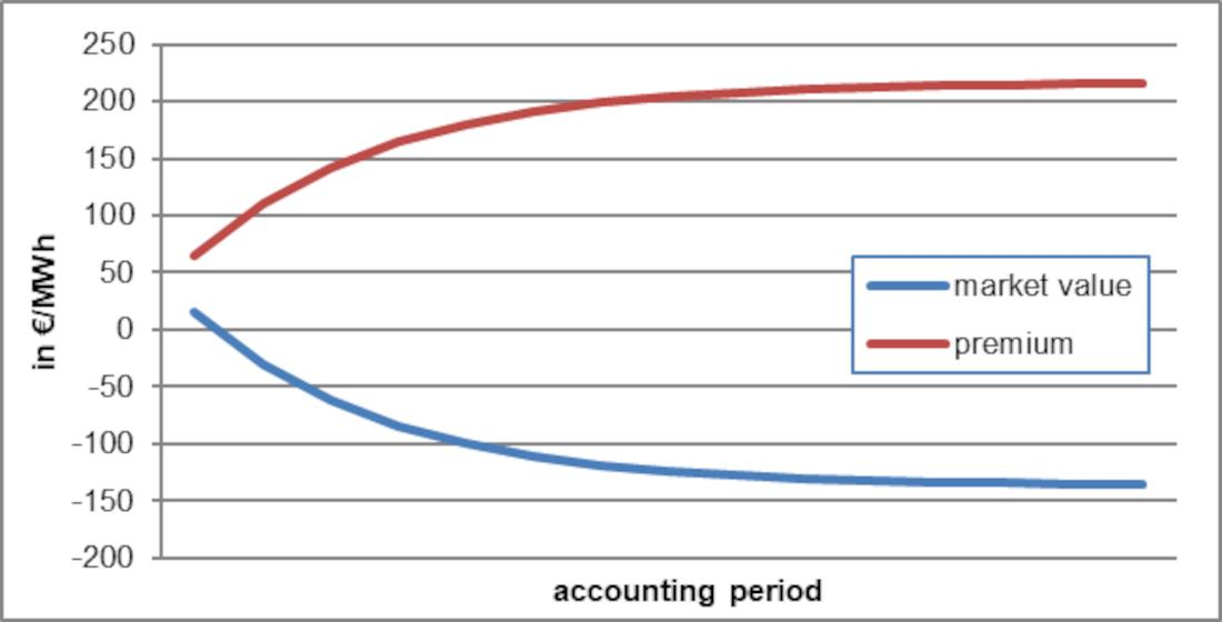
A recursive relation between the market premium and its value in the previous accounting period. Assuming there is a limit of this sequence it can be calculated by setting , which yields
The interested reader can prove that the sequence is finite and monotone, which proves that is indeed the sequence’s limit, i.e., Inserting into Equation (2) allows to calculate the stable market value . Using the same marginal costs and levelized cost as in case 1 (no market impact) and a fraction for technology N to set the market price, the market premium quickly converges to about . The average market price per accounting period then stabilizes at roughly . This is significantly lower than , which would be the market value without any market premium. The latter value can be obtained by setting in Equation (2). Thus, at low fractions , the policy instrument already has a moderate impact on the average market prices. Note that these results are independent from the initial choice of , which only affects the time necessary to reach convergence. If , the system stabilizes immediately. For simplicity, we choose .
3.1.3. Case 3: Significant Market Distortion
In case that technology N is price setting for a significant fraction of each accounting period, the recursive relation (Equation (3)) dominates market behavior and a self-reinforcing feedback loop of declining market prices is set in motion. Using the same values for marginal costs and levelized cost as in the previous cases, but assuming that , market values would converge at about and the market premium would be as high as . This is caused by the fact that the offers of technology N account for the expected market premium. However, at times where technology N is price setting, this strategy yields no revenues. As a consequence, the market premium is increased at the end of each such accounting period to ensure that technology N recovers its costs. This, however, leads to even lower offers of technology N in the next accounting period and a further market value decline.
Finally, the market values and premia will converge to the aforementioned limits as long as . These converged market values stand in stark contrast to market values without premia. In such a case, the market price would be much higher; in this example . Thus, under these circumstances the policy instrument distorts the market significantly.
3.2. Results from the Agent-Based Simulation
3.2.1. Results for the Simple Scenario
To illustrate the results of the bidding behavior in a simplified electricity market for VRE described above in Section 2.2, a simple scenario with the agent-based modelling simulation software AMIRIS was set up in order to prove the general validity of the effect. The only two electricity generation technologies (see Table 1) were photovoltaic (PV, 200 GW) and gas (120 GW) and a carbon price of 0 €/t was chosen. Gas power plants’ marginal cost were fixed at 47.13 €/MWh.
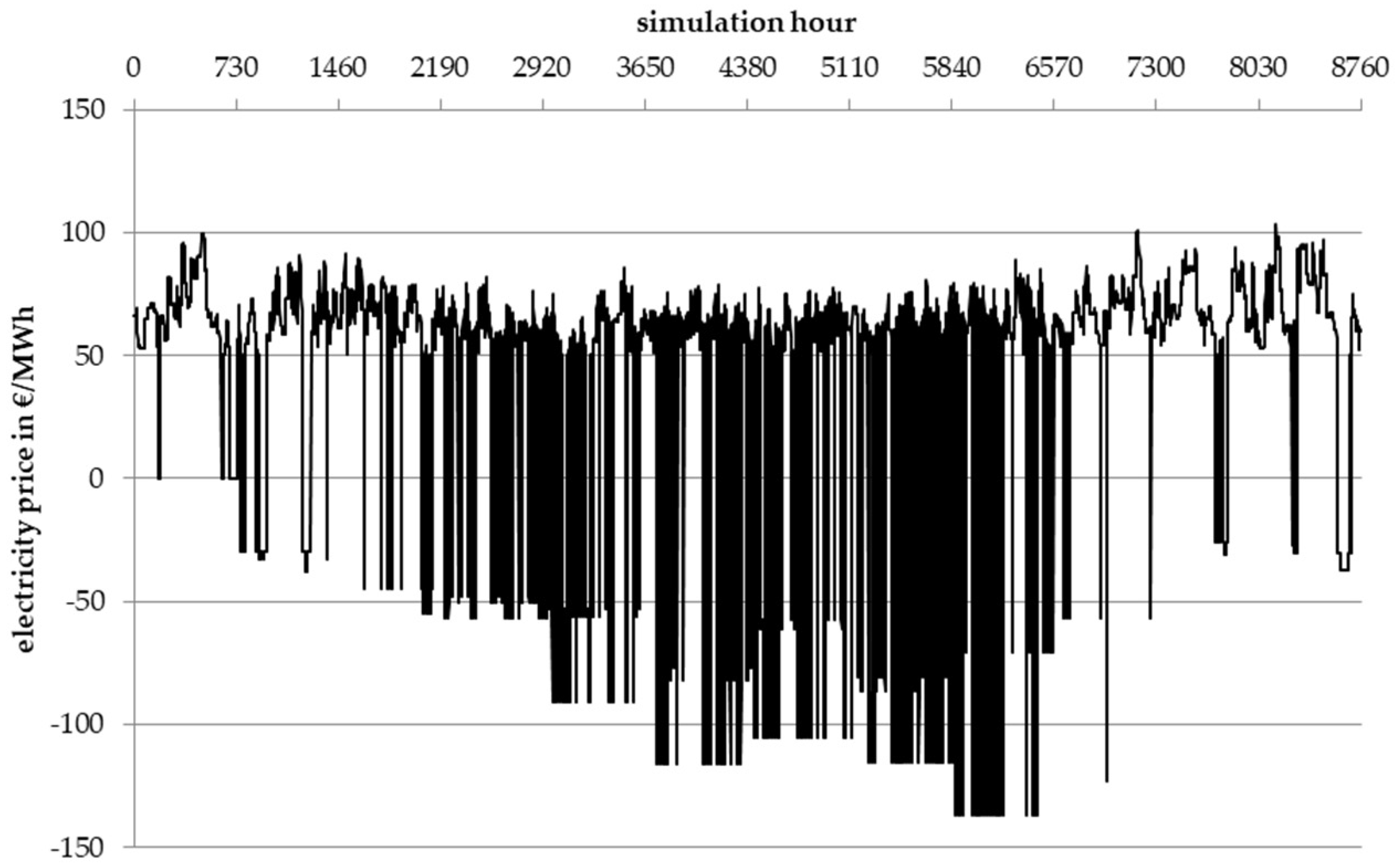
The resulting market prices in this scenario are shown in Figure 1. The highest prices for electricity amounted to 47.13 €/MWh which was the marginal cost of the gas fired plants. In the first and last 2 months of the simulation year (which consisted of 8760 h, each month of 730 h), there were no hours with a negative residual load. The residual load was defined as the difference between actual power demand and the feed-in of non-dispatchable and inflexible generators [28]—in this case PV. As long as PV could not cover the entire load, gas power plants remained price setting due to the merit order [29,30] in the assumption of a uniform pricing at the energy market, where all accepted bids were paid the same market clearing price [31,32].
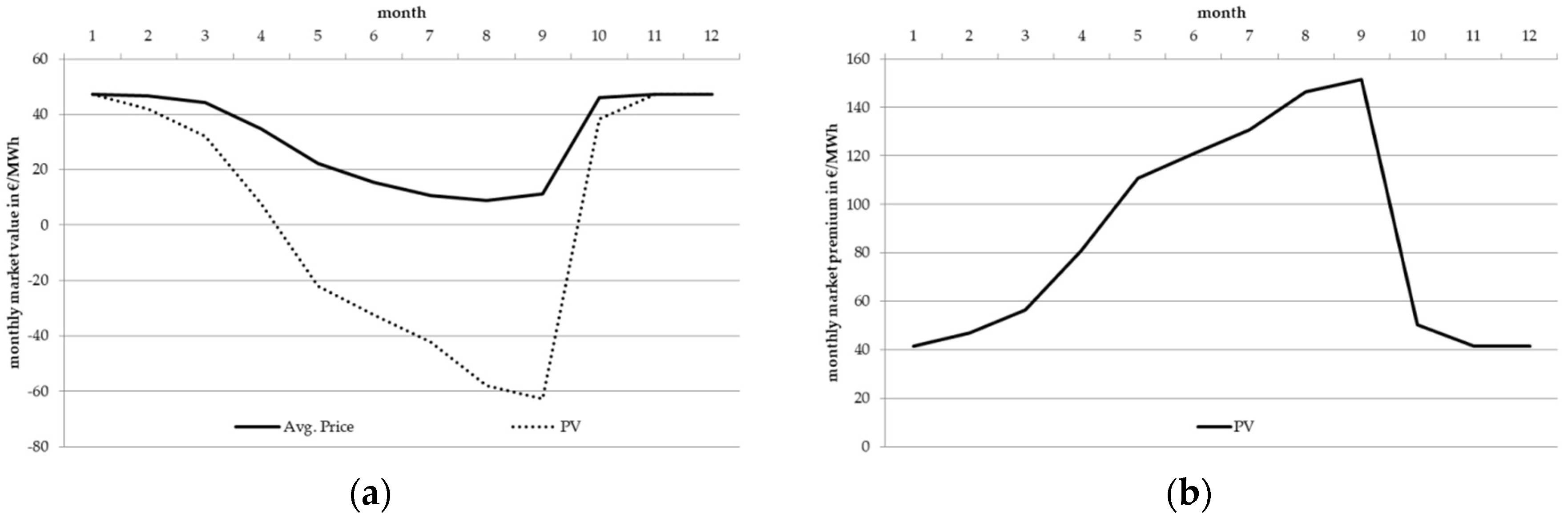
However, towards the end of the second month, PV became load-balancing and was price setting for five hours. Bids were placed at −41.46 €/MWh, resulting in an equivalent price for these hours. The underlying calculation was anticipating the market premium to match the effective premium of the previous month. Since in the previous month the electricity price was constantly at 47.13 €/MWh, so was the market value of PV (Figure 2a). The assumed LCOE of PV, i.e., the cost of the production of a megawatt-hour levelized over the lifetime of a plant, amounted in the simulation to 88.6 €/MWh. Hence, the market premium in the first month covered the gap of 41.46 €/MWh between LCOE and market value (Figure 2b). To maximize the chances of being awarded (and acquiring the premium) bids were set to equal the marginal cost minus the anticipated market premium. With marginal costs of 0 €/MWh and a previous month’s premium of 41.46 €/MWh this resulted in the aforementioned (price-setting) bids of −41.46 €/MWh.
Due to these five hours with negative prices in month 2, the monthly average market value of PV decreased to 41.80 €/MWh for this month. Since the market premium had to compensate for this, it increased to 46.79 €/MWh. Again, this value served as basis for the PV bid calculation in the following month. Thus, PV-bids in the third month were calculated with marginal costs of 0 €/MWh minus the increased market premium of 46.79 €/MWh, resulting in bids at −46.79 €/MWh.
With increasing hours of load-balancing PV feed-in the prices decline month by month, since the market premium was adjusted monthly and reflects the ongoing decreasing market value of PV (see Figure 2). This effect is also referred to as “cannibalization effect” [33]. This decline continued as long as PV covered the demand in such a significant share of the monthly hours that its market value kept declining. In autumn, PV was increasingly unable to cover the load (in the month 10 it is load-balancing for only 5 h), gas became price-setting in most cases and the market value for PV increased steeply. The market premium was adjusted and fell accordingly.
These results reveal self-reinforcing negative price-dynamics under the variable market premium scheme in the case of high VRE shares. Hence, the results of a simplified scenario of an established, agent-based electricity market model confirm the discovered effect and the results of the mathematical model.
3.2.2. Results for the Extended Scenario
To examine whether the effect is also observable in a more realistic setting, an extended scenario was developed for a prospective German electricity system with a high share of VRE. The technological scenario parameters are shown in Table 2.
Apart from the high share of renewables, the scenario was deliberately generic reflecting typical characteristics of scenarios with high shares of renewables. It was not modelled for a certain year, since its purpose was to show that the price dynamics discussed will also set in more realistic market settings with different technologies. Further scenarios with different compositions of power plant technologies were conducted (a scenario with high wind capacity and one with high storage capacities are shown in Appendix A (Appendix A.2 and Appendix A.3)).
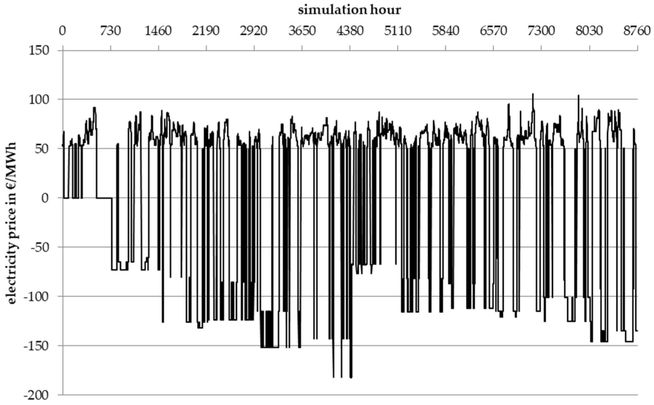
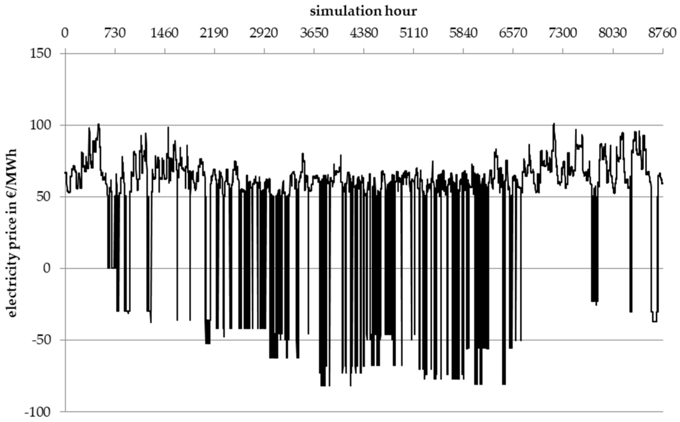
The resulting electricity prices for one year in the extended scenario are displayed in Figure 3. They fluctuate much more than in the simple scenario. Yet, the same pattern of monthly stepwise decreasing market prices until the end of summer is evident.
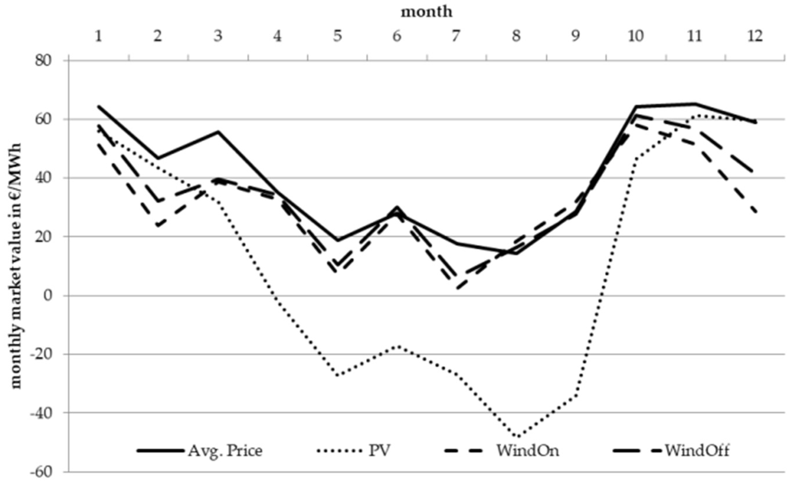
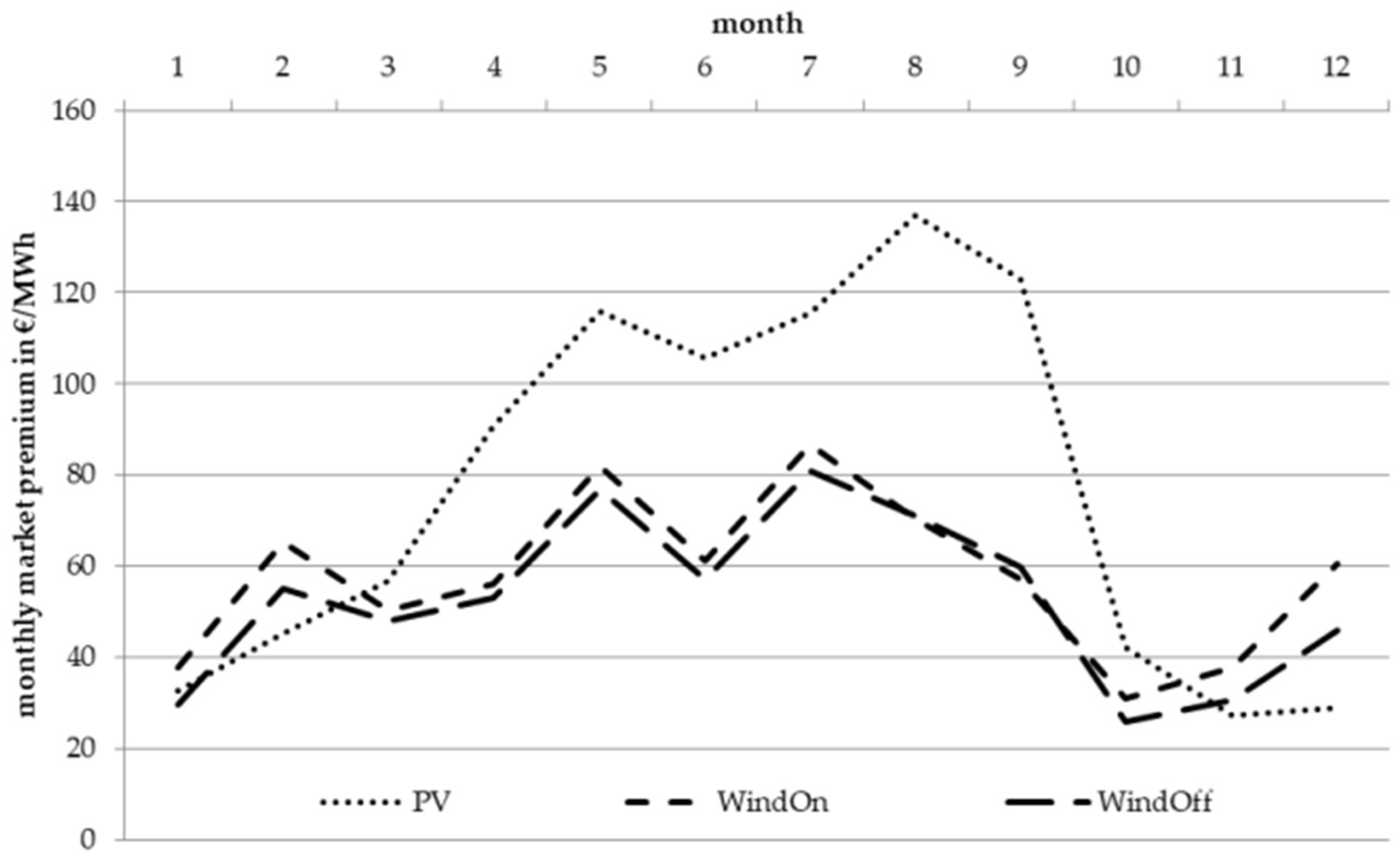
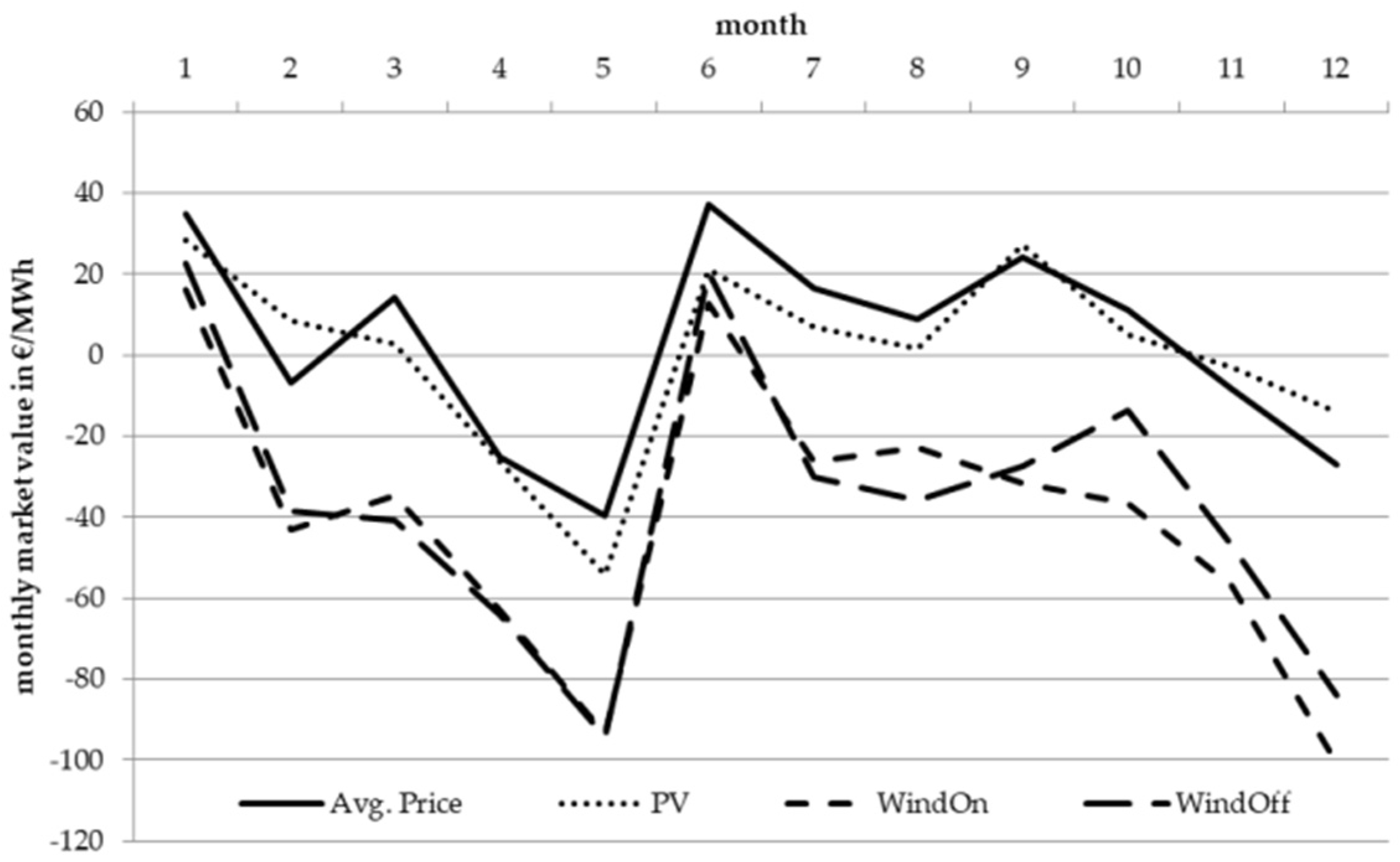
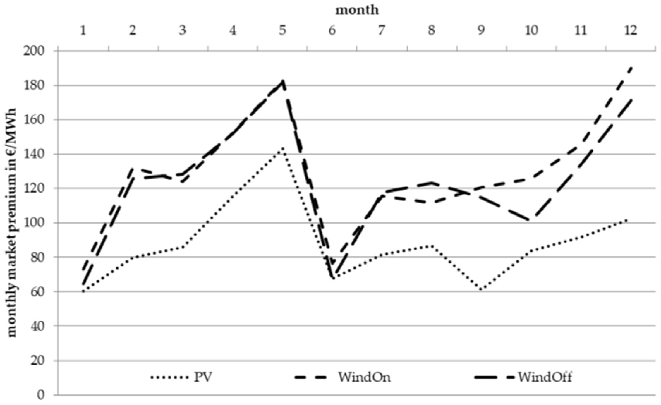
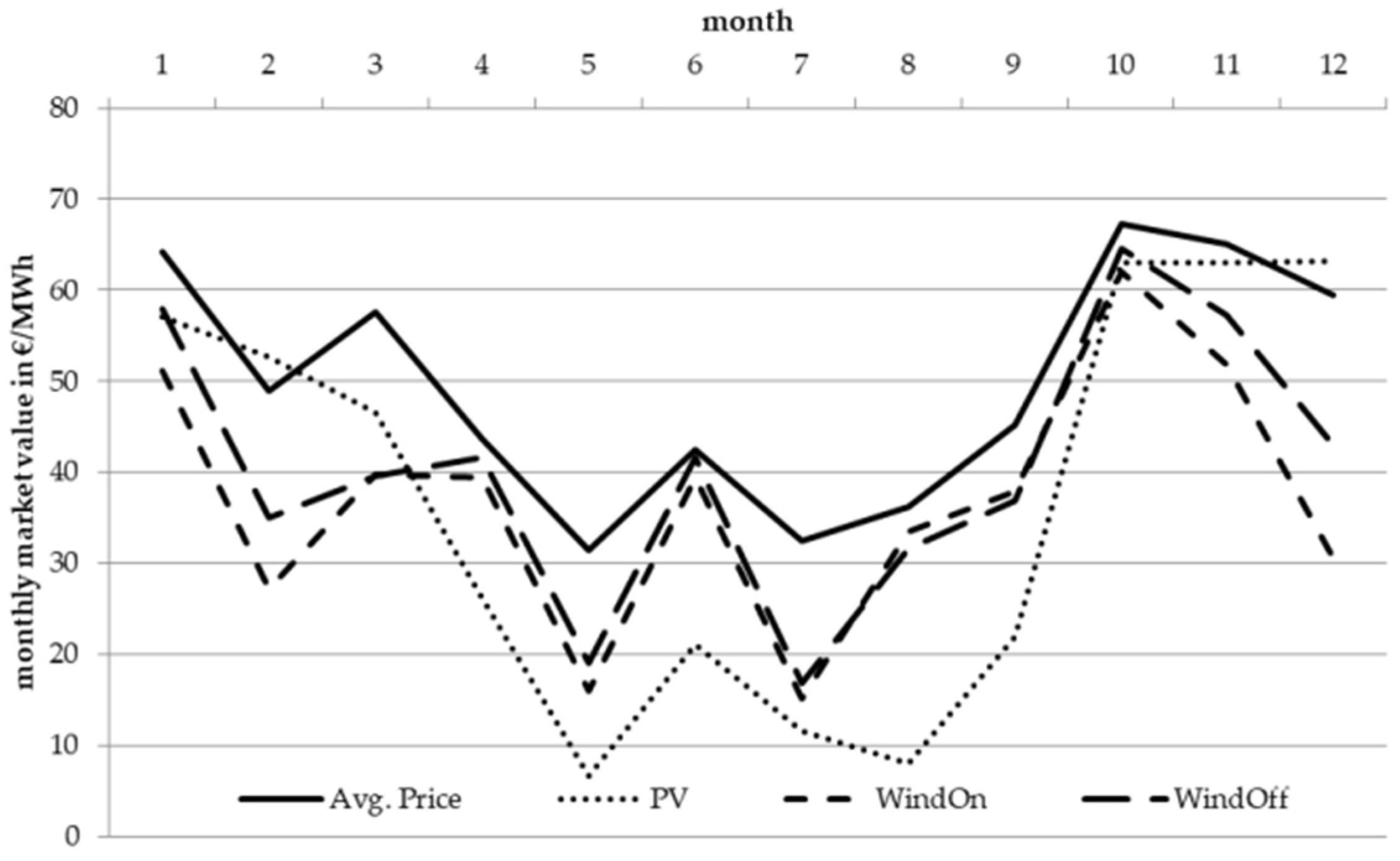
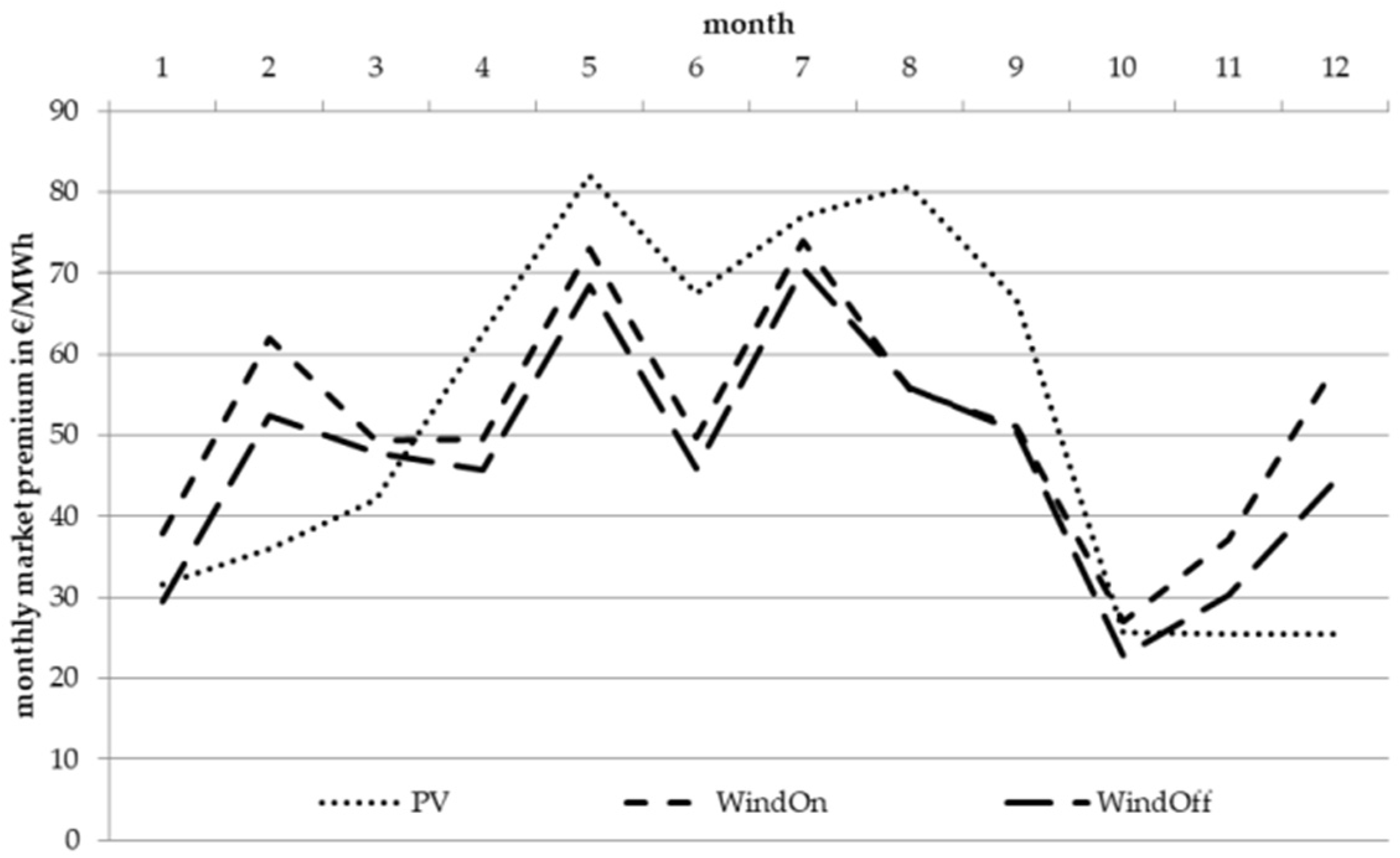
Like in the simple scenario, conventional technologies dominated the market in the first month. However, for about 59 h VRE could cover the load. Similar to the mathematical model, the agents anticipated a market premium of 0 €/MWh in the first month of the simulation. Therefore, their bid equaled their marginal cost of 0 €/MWh. For this first month with a relatively high average electricity price level of 64.36 €/MWh the value of the market premium was calculated ex post to 37.91 €/MWh for wind onshore, 29.70 €/MWh for wind offshore, and 32.73 €/MWh for PV (Figure 4 and Figure 5). Consequently, corresponding negative prices occurred in the second month, because VRE technologies adjusted prices according to these values and are price-setting in 165 simulation hours. In the following, again, the decline of market prices could be observed over the summer months.
In addition, the development of market values and the monthly adjusted variable market premium in the extended scenario revealed a strong influence between different renewable energy technologies. This has been referred to as cross-cannibalization effect [33].
In essence, for PV, the results were very similar to those of the simple scenario. The LCOE were not covered by the monthly average market value in the beginning of the year. Hence, the market premium had to compensate for the difference. The PV-driven price dynamic gained momentum in month 4, where PV became price-setting for 42 h. However, together with another 101 h, in which wind technologies covered the load, these 143 h covered 54% of the electricity fed-in by PV in that month (Table 3).
As PV feed-in was more synchronous than wind, market values of PV decreased faster in comparison. In month 4, this led to bids of −56.78 €/MWh, which were below both wind on- (−50.44 €/MWh) and offshore (−47.78 €/MWh) bids. This position at the lower end of the merit order was kept until month 11. During this period, PV was awarded in every hour it bid, either at self-imposed prices, or at those from wind and conventional technologies.
Since wind also bid negatively, the market value of PV decreased even more, compared to a single-technology system like the simple scenario in Section 3.2.1. In contrast, the effective market value of wind energy being sold was not influenced by the bids of PV from month 4 to month 11, as PV price-setting hours pushed wind out of the market, resulting in decreasing full load hours for wind. Nevertheless, hours with potential wind feed-in were considered when calculating the reference market value for the market premium, thus they increased the market premium for wind. In the same period, though, the share of wind onshore feed in within VRE price-setting hours was at 18% and for wind offshore at 6%. In contrast to the much more synchronous feed in of PV, the pattern for wind was clearly more inhomogeneous and market values for wind did not decrease as fast. This effect stopped in autumn, when price-setting hours were getting scarcer (20 h for VRE in month 10) and market values subsequently rose.
To measure these cross effects, our simulations allow us to calculate the “market share cross influence” as the share of production technology A (here: PV, wind onshore or wind offshore) in hours where technology B (here: PV on the left-hand side or wind onshore on the right-hand side of Table 4) is price setting in total awarded production of A (Table 4).
In summary, we report that the extended scenario showed the same pattern of increasing negative electricity prices as both the simple scenario and the mathematical model. This result was supported by scenarios with a high share of wind or storage capacity (see Appendix A.2 and Appendix A.3). The mechanism described depended on the variable market premium and the strategic bidding behavior of PV and wind marketers and was enhanced by cross-effects between these two different technologies. In hours with a negative residual load, PV and wind became price-setting. Their strategic bidding behavior, i.e., bids at marginal cost minus the variable market premium, drove prices down. With decreasing prices, the average monthly market values for PV and wind started to decline (Figure 4). The variable market premium was increased to cover the LCOE (Figure 5). PV and wind bids included this increased premium in their next calculations and prices became even more negative. Hence, this downward spiral continued as a self-reinforcing effect as long as these technologies were price-setting at a significant share of hours per month. The next section discusses possible solutions for this effect.
4. Discussion
Now that self-reinforcing deflationary price dynamics under the variable market premium scheme have been mathematically described and shown to be persistent in more realistic market simulations, one question emerges—is this effect of practical relevance? We identify three categories of objections: deflationary price dynamics will not occur in this form, since the effect…
- … is an artefact of the simulation itself (Objection A);
- … is attenuated by other influences (Objection B);
- … is already addressed by current regulations (Objection C).
4.1. Objection A—Is the Effect a Model Artefact?
Both the mathematical model and the simulations are simplified examples—hence the effect observed could be due to model artefacts. One assumption is that remunerated plant operators are willing to offer energy at negative prices. Furthermore, to determine their (negative) bidding prices, a simplistic forecast of the expected market premium has been used. Although doubts regarding these two aspects of the modelling are legitimate, we will show that these are, in fact, sound assumptions.
The basis for the assumption of plant operators bidding at negative prices is the guaranteed income via the market premium. The premium fills the gap between a plant operator’s income from the electricity market and its LCOE, provided the plant operator’s feed-in pattern matches the average feed-in pattern of the corresponding technology. Since the subsequent balancing of market revenues to the LCOE is guaranteed, negative bidding is virtually risk-free: If the plant operator is price-setting, any occurring losses due to negatives bids are compensated for by the market premium. At the same time, this strategy increases the probability of being awarded in the spot market and thus increases the amount of claimable premia.
Therefore, market participants who offer energy at variable marginal costs without considering markdowns have a higher volume risk and their bidding strategy should be evolutionarily unstable [34]. In theory, bids can be as negative as permitted by the lower price limit of the energy exchange. However, if a significant share of plant operators places substantially lower bids than their competitors, the income of the latter may be increased beyond their corresponding LCOE. This is caused by a disproportionate increase of the market premium rewarded to the competitors compared to their reduced market share. Consequently, a bidding strategy that employs the expected market premium as bidding price offers a reasonable compromise between these two risks.
Hence, the fundamental problem described exists independently of our simplifying assumptions. Decreasing prices are offset by the premium and using the expected premium as bidding price is a reasonable strategy [35].
This leads to a second possible objection: The forecast of the expected market premium shows a significant impact on the models’ convergence behavior. Nevertheless, the simplified estimate of the market premium equaling that of the previous accounting period is used. It is likely that real-world actors would make more of an effort to obtain more precise estimates for the expected market premium. Possible methods could include adjustments of the expected value during the accounting periods or to use information from previous years to better reflect the premium’s dynamics during a year.
However, more sophisticated forecasts do not have any impact on the general dynamics of the market premium that we report. Equations (3) and (4) offer but one point of stability, i.e., where the expected market premium equals the actual one. Thus, on the contrary, if prediction methods for the expected market premium are enhanced, this will only lead to a faster convergence of the system.
In summary, both objections do not hold. Either they do not concern the general dynamics or they would even aggravate the problem.
4.2. Objection B—Is the Effect Attenuated by Other Influences?
Yet, both the plain mathematical model and the AMIRIS simulation are stylized and simplified. Therefore, they possibly abstract away important features of the real world that may counteract the strong decline in market prices and market values of VRE described above. In the following, it is discussed which factors might counteract this effect of declining prices.
For example, the chosen scenario, due to its relatively strong PV deployment, may overestimate the self-reinforcing effect. Especially in summer, synchronous production profiles enhance the share of hours where PV is price setting. This decreases prices and thus market values even stronger. We can confirm the strong influence of PV on the results in our simulations.
However, we observe the deflationary price dynamics in scenarios with large wind capacities as well. This result is robust against different proportions of technologies, since we conducted several sensitivity checks regarding the influence of the composition of the power plant park (for a scenario with high wind capacities see Appendix A.2).
Scenarios with large wind capacities reveal cross effects like in the extended scenario above—just with wind as price-dominating technology. Hours with alternative price-setting technologies with negative bids and differing feed-in profiles further reduce the market values of the technologies considered. Hence, the deflationary effects of the different technologies reinforce each other.
A further argument could be that these effects are attenuated by expanding storage capacities. We examined this sensitivity, too. Storage capacities are included in the expanded scenario with 20 GW capacity at an energy to power-ratio of 7. In an alternative scenario, the capacity was increased to 40 GW. As expected, increasing storage capacities reduces the number of hours in which renewables bidding with negative prices are price-setting. Accordingly, monthly averages of electricity prices and thus market values of PV and wind are higher; this, in turn, results in lower market premia. However, the deflationary dynamics occur even with these highly ambitious assumptions in place (for a scenario with high storage capacities see Appendix A.3).
It could further be argued that future energy systems with high shares of VRE very likely face higher demand as a result of increased sector coupling. For instance, a new demand may arise from P2X technologies like power-to-heat, power-to-gas and power-to-vehicle technologies. These technologies transfer electrical energy into other energy sectors. Consequently, PtX technologies have the potential to significantly reduce the amount of hours with negative or zero prices assuming a certain “willingness-to-pay” for these applications [36]. For the price-declining effect to occur, however, a correspondingly high proportion of VRE is essential. Accordingly, growing demand will only delay the effect, but not cancel it.
Finally, import and export of electric power is not considered in the simulation. In case of a meteorological condition that leads to a high VRE electricity production in one country and a small VRE electricity production in a neighboring country and resulting price differences, electricity would be traded across borders. This leads to lower prices in the importing country and to higher prices in the exporting country, thus reducing the probability of negative prices in the market.
Cross-border trade adds flexibility to a country’s market and could therefore mitigate the discussed market price declining effect if weather patterns are sufficiently decorrelated. Even today there are situations when residual loads are low in much of continental Europe, as for example on the 5th of July 2020. On that date, day-ahead prices in all Central Western Europe were negative during the whole day.
We therefore believe that it is unlikely that these, or the other influences discussed can cancel the effect completely.
4.3. Objection C—Is the Effect Addressed by Current Regulations?
Finally, market price decline might be limited by instruments and regulatory design itself. For instance, the so called 6-hour-negative pricing rule has been implemented in the renewable energy source act 2014 in Germany [37]. Its aim is to incite curtailment in hours of overproduction. Therefore, this regulation ensures that the market premium is set to zero if prices at the day-ahead auction are below zero in 6 and more consecutive hours.
Obviously, this regulation prevents the observed effect. At the same time, it significantly reduces potential full-load hours of renewables with corresponding substantial risks for their refinancing. In fact, this negative impact can already be observed at present. For instance, an estimated €50 million in losses for offshore wind projects in February 2020 alone have been attributed to this regulation [38]. While the declining price effect is thus prevented at present, this adjustment would significantly impact in a negative way on the refinancing for an electricity system with a high proportion of VRE in the long term.
Another regulative solution would be to cap premia at a maximum value, for example at the LCOE in order to still be able to ensure refinancing. This approach has at least two disadvantages: (a) it will hardly be possible to calculate the LCOE correctly if the foreseeable changes in full-load hours are considered, and (b) relatively expensive technologies are placed to the left of the cheaper technologies in the merit order. Both problems mean that a new market distortion emerges. This would significantly weaken the function of the market to ensure an efficient allocation of resources.
Yet another regulation that would prevent the declining price effect is the introduction of a fixed market premium, which has been used, e.g., in Germany for the so-called innovation tenders [39]. With this design, the premium is independent of the market price. The premium is a constant payment in addition to the market price which is effected at the market. Hence, the variation in returns depends strongly on market price variations. However, this has the drawback that the refinancing of plant owners is exposed to a significantly higher risk [40].
Finally, an alternative design of the market premium, which is, for example, in place in Great Britain and France for offshore wind, are so-called contracts for difference (CFD, also referred to as symmetrical market premium or double-sided sliding premium) [15,16]. If the average market value is below the CFD value, the plant operator receives this difference as a premium. If the market value is above the CFD value, the plant operator pays the difference to the counterparty. While this mechanism prevents excessive profits to power plant operators, the declining price effect remains the same as for the variable market premium, since the contract covers the price risks.
We conclude that the regulations discussed above would indeed prevent the self-reinforcing downward electricity price dynamics. However, they all have undesired side effects.
5. Conclusions
Both a plain mathematical model and two scenarios with the agent-based simulation model AMIRIS show that high shares of fluctuating renewables in combination with variable market premia may lead to a downward spiral of electricity prices and increasing costs for their support.
We are convinced that there is a basic problem: Market premia play an essential role in the market integration of renewables by guaranteeing investment security and aligning production with demand. However, at very high shares of fluctuating renewables they distort the market price formation, which results, in the worst case, in a self-reinforcing loop of declining prices. If technologies that receive an ex-post market premium cover 100% of consumption and thus become price-setting, they counteract an effective and efficient further integration of renewables. Price-setting power plants may demand any negative price and are remunerated with a market premium in any case, since this instrument has been designed to guarantee refinancing in accordance with the value to be invested. Hence, the main driver for the discussed downward loop consists in premia filling in even for negative prices. Since premium recipients are by design retroactively remunerated with a reference value and can thus call up virtually any prices, the mechanism can be exploited under certain circumstances.
High negative prices could be one result of this negative feedback loop. These would have unfavorable effects on the electricity market and the electricity system as a whole. First, they would distort the level of market prices and thus offer false incentives for the operation and investment of generation technologies as well as demand. Second, acceptance of technologies receiving premia could be reduced by a strong price influence; electricity prices would certainly fall, but the remuneration costs paid by electricity customers would skyrocket at the same time. Distribution effects also have to be considered—e.g., in Germany, not all electricity consumers are equally involved in the payment of remunerations.
The described dilemma is not trivial to avert in the current market setting, as voluntary change in bidding behavior is not to be expected. The problem is also not easy to circumvent given the current remuneration system. However, a direct intervention in the market (e.g., prohibiting negative bids) would indeed avoid the self-reinforcing pattern described above. Yet, it is to be expected that refinancing of premium recipients would then be in jeopardy. Yet, refinancing is one of the main reasons for market premia to exist in the first place. Fixed market premia would also entail immense investment risks for the state given very high levels of VRE. In addition, this would jeopardize refinancing of newcomer plants, as do upper and lower limits for the variable market premium.
Since many countries employ feed-in premia (see above), and VRE are increasing their share, such potential downward price spirals might become problematic on a larger scale. Hence, we conclude that this problem needs further investigation and encourage the research community to reproduce our findings. We need solutions for both how the refinancing of new technologies and efficient allocation of electricity generation at the wholesale market can work at high shares of renewable energy. One interesting aspect to study is to calculate the point—both from a national or European point of view and of the individual actors involved—when it would be optimal to stop giving market premia to renewables and switch to other support instruments like capacity mechanisms or quota systems for VRE.
Author Contributions
Conceptualization, M.K. and C.S.; formal analysis, M.K. and C.S.; data curation, K.N., U.J.F, C.S; writing—original draft preparation, M.K., U.J.F., K.N., and C.S.; writing—review and editing, U.J.F., K.N., and C.S. All authors have read and agreed to the published version of the manuscript.
Funding
This research was funded by the Bundesministerium für Bildung und Forschung, grant number 03SFK4D1 and the Bundesministerium für Wirtschaft und Energie, grant number 03ET4020.
Acknowledgments
We acknowledge the very valuable help and feedback of Marc Deissenroth.
Conflicts of Interest
The authors declare no conflict of interest.
Appendix A
Appendix A.1. Details on AMIRIS
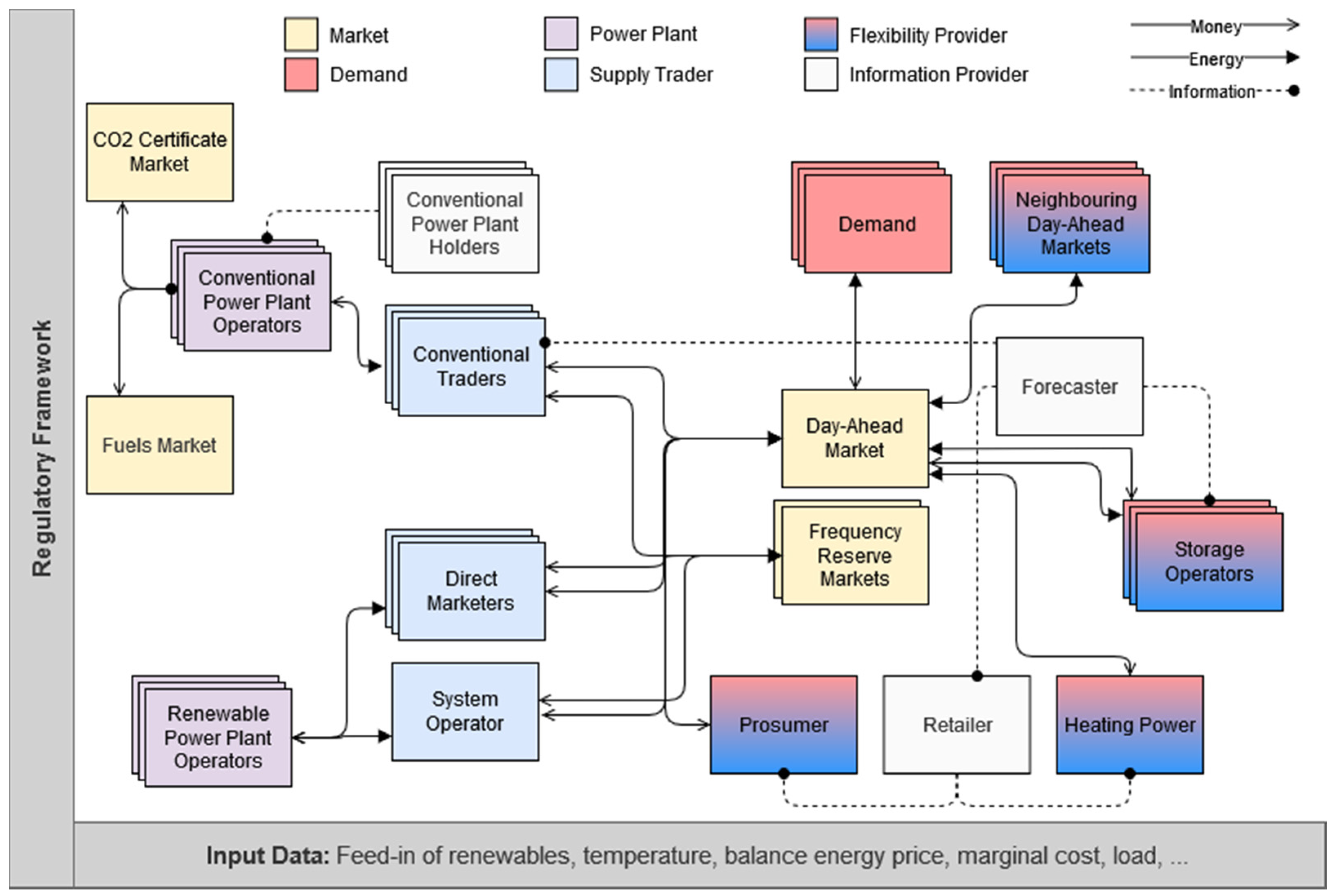
Figure A1 depicts the communication of agents in the full AMIRIS model. Communication takes place in the same way for each simulated hour: All plant operators send expected electricity production quantities (with deliberate estimation errors) to their contractual electricity traders (direct marketers or grid operators). Based on these expected electricity quantities and associated marginal costs, the traders generate bids which are transmitted to the day-ahead power exchange.
The power exchange evaluates the bids of all electricity suppliers, electricity consumers and storage operators, calculates the merit order and the equilibrium price and then sends or requests the money for accepted bids.
Subsequently, the network operators pay the feed-in tariff due to their clients. The direct marketers can grant their contractually linked plant operators an additional bonus. This bonus depends on the income from the market for negative minute reserve (control energy market), the claims of market premiums, and the costs for balancing energy.
The storage operators have a special role in AMIRIS in so far as they can carry out arbitrage transactions as independent traders on the energy exchange on the one hand, but can also be used by direct marketers to reduce the balancing energy demand caused by forecasting errors on the other hand [21].
Figure A1.
AMIRIS model scheme.

The agent-based simulation AMIRIS is heavily based on the Open-Source framework FAME. It is available at GITLAB at https://gitlab.com/fame2. It consists of the core files (FAME-core), a demo (FAME-demo), a data input and scenario generator tool (FAME-py) and a documentation (FAME-wiki).
Appendix A.2. Scenario with High Wind Capacities

Table A1.
Scenario parameters for the technologies in the extended scenario.
| Technology | Capacity/GW |
|---|---|
| Photovoltaics | 100 |
| Wind Onshore | 180 |
| Wind Offshore | 40 |
| Gas CC | 35 |
| Gas Turbine | 20 |
| Hard Coal | 15 |
| Lignite | 10 |
| Storage 1 | 20 |
1 Energy to Power Ratio = 7.
Figure A2.
Market prices for one year in the extended wind scenario.

Figure A3.
Development of market values for PV, wind onshore and wind offshore in the extended wind scenario.
Figure A3.
Development of market values for PV, wind onshore and wind offshore in the extended wind scenario.

Figure A4.
Development of the market premium for PV, wind onshore and wind offshore in the extended wind scenario.
Figure A4.
Development of the market premium for PV, wind onshore and wind offshore in the extended wind scenario.

Appendix A.3. Scenario with High Storage Capacities
Table A2.
Scenario parameters for the technologies in the extended storage scenario.
| Technology | Capacity/GW |
|---|---|
| Photovoltaics | 200 |
| Wind Onshore | 80 |
| Wind Offshore | 20 |
| Gas CC | 35 |
| Gas Turbine | 20 |
| Hard Coal | 15 |
| Lignite | 10 |
| Storage 1 | 40 |
1 Energy to Power Ratio = 7.
Figure A5.
Market prices for one year in the extended storage scenario.

Figure A6.
Development of market values for PV, wind onshore and wind offshore in the extended storage scenario.
Figure A6.
Development of market values for PV, wind onshore and wind offshore in the extended storage scenario.

Figure A7.
Development of the market premium for PV, wind onshore and wind offshore in the extended storage scenario.
Figure A7.
Development of the market premium for PV, wind onshore and wind offshore in the extended storage scenario.

References
- BMWi. Zeitreihen zur Entwicklung der Erneuerbaren Energien in Deutschland 1990–2018; Bundesministerium für Wirtschaft und Energie: Berlin, Germany, 2019. [Google Scholar]
- IEA. World Energy Outlook 2019. 2019. Available online: https://www.iea.org/reports/world-energy-outlook-2019 (accessed on 8 October 2020).
- Eurostat. Eurostat European Statistics Database; Eurostat: London, UK, 2018. [Google Scholar]
- Teske, S. Achieving the Paris Climate Agreement Goals: Global and Regional 100% Renewable Energy Scenarios to Achieve the Paris Agreement Goals with Non-Energy GHG Pathways for +1.5 °C and +2 °C; Springer: Cham, Germany, 2019. [Google Scholar]
- Jacobson, M.Z.; Delucci, M.A.; Bauer, Z.A.F.; Goodman, S.C.; Erwin, J.R.; Fobi, S.N.; Liu, J.; Lo, J.; Meyer, C.B.; Morris, S.B.; et al. 100% Clean and Renewable Wind, Water, and Sunlight All-Sector Energy Roadmaps for 139 Countries in the World. Joule 2017, 1, 108–121. [Google Scholar] [CrossRef] [Green Version]
- Brown, T.W.; Blok, K.; Breyer, C.; Lund, H.; Mathiesen, B.V. Response to ‘Burden of proof: A comprehensive review of the feasibility of 100% renewable-electricity systems’. Renew. Sustain. Energy Rev. 2018, 92, 834–847. [Google Scholar] [CrossRef]
- Winkler, J.; Giao, A.; Pfluger, B.; Ragwitz, M. Impact of renewables on electricity markets—Do support schemes matter? Energy Policy 2016, 93, 157–167. [Google Scholar] [CrossRef]
- Purkus, A.; Gawel, E.; Deissenroth, M.; Nienhaus, K.; Wassermann, S. Market integration of renewable energies through direct marketing—Lessons learned from the German market premium scheme. Energy Sustain. Soc. 2015, 5. [Google Scholar] [CrossRef] [Green Version]
- Alberici, S.; Boeve, S.; Deng, Y.; Wouters, K.; Winkei, T. Subsidies and Costs of EU Energy: Final Report. 2014. Available online: https://ec.europa.eu/energy/sites/ener/files/documents/ECOFYS%202014%20Subsidies%20and%20costs%20of%20EU%20energy_11_Nov.pdf (accessed on 8 October 2020).
- Mora, D. Auctions for Renewable Energy Support—Taming the Beast of Competitive Bidding: Final Report of the AURES Project. 2017. Available online: http://auresproject.eu/sites/aures.eu/files/media/documents/aures-finalreport.pdf (accessed on 8 October 2020).
- RESLEGAL. RES LEGAL Europe Comparison Tool. 2020. Available online: http://www.res-legal.eu/ (accessed on 8 October 2020).
- REN. Renewables 2017 Global Status Report. 2017. Available online: http://www.ren21.net/status-of-renewables/global-status-report/ (accessed on 8 October 2020).
- Klobasa, M.; Ragwitz, M. Market Integration of Renewable Electricity Generation—The German Market. Premium Model. Energy Environ. 2013, 24, 127–146. [Google Scholar] [CrossRef]
- Kitzing, L.; Weber, C. Support. mechanisms for renewables: How risk exposure influences investment incentives. Int. J. Sustain. Energy Plan. Manag. 2015, 7. [Google Scholar] [CrossRef] [Green Version]
- Pollitt, M.G.; Anaya, K.L. Can current electricity markets cope with high shares of renewables? A comparison of approaches in Germany, the UK and the State of New York. Energy J. 2016, 37. [Google Scholar] [CrossRef] [Green Version]
- Neuhoff, K.; May, N.; Richstein, J.C. Renewable Energy Policy in the Age of Falling Technology Costs. 2018. Available online: http://hdl.handle.net/10419/181032 (accessed on 8 October 2020).
- Visser, E.; Held, A. Methodologies for Estimating Levelised Cost of Electricity (LCOE); Ecofys: Utrecht, The Netherlands, 2014. [Google Scholar]
- Newbery, D.; Pollitt, M.G.; Ritz, R.A.; Strielkowski, W. Market design for a high-renewables European electricity system. Renew. Sustain. Energy Rev. 2018, 91, 695–707. [Google Scholar] [CrossRef] [Green Version]
- Cramton, P.; Stoft, S. Why We Need to Stick with Uniform-Price Auctions in Electricity Markets. Electr. J. 2007, 20, 26–37. [Google Scholar] [CrossRef] [Green Version]
- Blume-Werry, E.; Faber, T.; Hirth, L.; Huber, C.; Everts, M. Eyes on the Price: Which Power Generation Technologies Set the Market Price? Price Setting in European Electricity Markets: An Application to the Proposed Dutch Carbon Price Floor. 2019. Available online: https://EconPapers.repec.org/RePEc:ags:feemes:281287 (accessed on 8 October 2020).
- Torralba-Díaz, L.; Schimeczek, C.; Reeg, M.; Savvidis, G.; Deissenroth-Uhrig, M.; Guthoff, F.; Fleischer, B.; Hufendiek, K. Identification of the Efficiency Gap by Coupling a Fundamental Electricity Market Model and an Agent-Based Simulation Model. Energies 2020, 13, 3920. [Google Scholar] [CrossRef]
- Reeg, M. AMIRIS—Ein Agentenbasiertes Simulations-Modell zur Akteursspezifischen Analyse Techno-Ökonomischer und Soziotechnischer Effekte bei der Strommarktintegration und Refinanzierung Erneuerbarer Energien; Technische Universität Dresden: Dresden, Germany, 2019. [Google Scholar]
- Deissenroth, M.; Klein, M.; Reeg, M. Assessing the Plurality of Actors and Policy Interactions: Agent-Based Modelling of Renewable Energy Market Integration; John Wiley & Sons: New York, NY, USA, 2017. [Google Scholar]
- Reeg, M.; Nienhaus, K. AMIRIS—Weiterentwicklung Eines Agentenbasierten Simulationsmodells zur Untersuchung des Akteursverhaltens bei der Marktintegration von Strom aus Erneuerbaren Energien unter Verschiedenen Fördermechanismen; DLR: Stuttgart, Germany, 2013. [Google Scholar]
- Klein, M.; Frey, U.J.; Reeg, M. Models Within Models—Agent-Based Modelling and Simulation in Energy Systems Analysis. J. Artif. Soc. Soc. Simul. 2019, 22, 6. [Google Scholar] [CrossRef]
- Reeg, M. AMIRIS—An Agent-Based Simulation Model for the Actor-Specific Analysis of Techno-Economic and Socio-Technical Effects in Electricity Market Integration and Refinancing of Renewable Energies; DLR: Stuttgart, Germany, 2019; Available online: https://nbn-resolving.org/urn:nbn:de:bsz:14-qucosa2-347643 (accessed on 8 October 2020).
- OPSD. Load, Wind and Solar, Prices in Hourly Resolution. 2020. Available online: https://data.open-power-system-data.org/time_series/2019-06-05 (accessed on 8 October 2020).
- Schill, W.-P. Residual load, renewable surplus generation and storage requirements in Germany. Energy Policy 2014, 73, 65–79. [Google Scholar] [CrossRef] [Green Version]
- Sensfuß, F.; Ragwitz, M.; Genoese, M. The merit-order effect: A detailed analysis of the price effect of renewable electricity generation on spot market prices in Germany. Energy Policy 2008, 36, 3086–3094. [Google Scholar] [CrossRef] [Green Version]
- Fischer, C. How can Renewable Portfolio Standards Lower Electricity Prices; Resources for the Future Discussion; RFF DP: Washington, DC, USA, 2006; pp. 6–20. [Google Scholar]
- Coase, R.H. The Economics of Uniform Pricing Systems. Manch. Sch. 1947, 15, 139–156. [Google Scholar] [CrossRef]
- Müsgens, F.; Ockenfels, A.; Peek, M. Economics and design of balancing power markets in Germany. Int. J. Electr. Power Energy Syst. 2014, 55, 392–401. [Google Scholar] [CrossRef]
- López Prol, J.; Steininger, K.W.; Zilberman, D. The cannibalization effect of wind and solar in the California wholesale electricity market. Energy Econ. 2020, 85. [Google Scholar] [CrossRef]
- Axelrod, R.; Hamilton, W.D. The evolution of cooperation. Science 1981, 211, 1390–1396. [Google Scholar] [CrossRef] [PubMed]
- Pahle, M.; Schill, W.P.; Gambardella, C. Renewable Energy Support. Negative Prices, and Real-time Pricing. Energy J. 2016, 37. [Google Scholar] [CrossRef]
- Brunner, C.; Möst, D. The impact of different flexibility options on future electricity spot prices in Germany. In Proceedings of the 12th International Conference on the European Energy Market (EEM), Lisbon, Portugal, 19–22 May 2015. [Google Scholar]
- EEG. Gesetz für den Ausbau Erneuerbarer Energien (Erneuerbare-Energien-Gesetz (EEG) Bundesanzeiger des Bundesministeriums für Justiz; BMVJ: Rostock, Germany, 2014. [Google Scholar]
- Knight, S. Six-Hour Negative Pricing Rule Damaging Offshore Wind Revenues; Windpower Monthly: London, UK, 2020. [Google Scholar]
- InnAusV. Verordnung zu den Innovationsausschreibungen (Innovationsausschreibungsverordnung—InnAusV); BMVJ: Rostock, Germany, 2020. [Google Scholar]
- Noothout, P.; de Jager, D.; Tesnière, L.; van Rooijen, S.; Karypidis, N.; Brückmann, R.; Jirouš, F.; Breitschopf, B.; Angelopoulos, D.; Doukas, H. The Impact of Risks in Renewable Energy Investments and the Role of Smart Policies; DiaCore: Athens, Greece, 2016. [Google Scholar]
Publisher’s Note: MDPI stays neutral with regard to jurisdictional claims in published maps and institutional affiliations. |
Figure 1.
Market prices for one year in the simple scenario.

Figure 2.
Level of the monthly market value (a) and of the variable market premium (b) for photovoltaic (PV) in the simple scenario.
Figure 2.
Level of the monthly market value (a) and of the variable market premium (b) for photovoltaic (PV) in the simple scenario.

Figure 3.
Market prices for one year in the extended scenario.

Figure 4.
Development of market values for PV, wind onshore and wind offshore in the extended scenario.
Figure 4.
Development of market values for PV, wind onshore and wind offshore in the extended scenario.

Figure 5.
Development of the market premium for PV, wind onshore and wind offshore in the extended scenario.
Figure 5.
Development of the market premium for PV, wind onshore and wind offshore in the extended scenario.

Table 1.
Scenario parameters for the technologies in the simple scenario.
| Technology | Capacity in GW |
|---|---|
| Photovoltaics | 200 |
| Gas Power Plant | 120 |
Table 2.
Scenario parameters for the technologies in the extended scenario.
| Technology | Capacity/GW |
|---|---|
| Photovoltaics | 200 |
| Wind Onshore | 80 |
| Wind Offshore | 20 |
| Gas CC | 35 |
| Gas Turbine | 20 |
| Hard Coal | 15 |
| Lignite | 10 |
| Storage 1 | 20 |
1 Energy to Power Ratio = 7.
Table 3.
Technology-specific share of monthly sold energy in hours when variable renewable energies (VREs) are price setting compared to monthly total of sold energy by that technology.
Table 3.
Technology-specific share of monthly sold energy in hours when variable renewable energies (VREs) are price setting compared to monthly total of sold energy by that technology.
| Month | PV | WindOn | WindOff |
|---|---|---|---|
| 1 | 14% | 17% | 10% |
| 2 | 24% | 43% | 23% |
| 3 | 20% | 24% | 21% |
| 4 | 54% | 18% | 6% |
| 5 | 62% | 28% | 19% |
| 6 | 46% | 11% | 3% |
| 7 | 59% | 31% | 14% |
| 8 | 65% | 15% | 7% |
| 9 | 52% | 7% | 13% |
| 10 | 15% | 3% | 3% |
| 11 | 7% | 15% | 6% |
| 12 | 4% | 35% | 11% |
Table 4.
Market share cross influence caused by PV (a) and wind onshore respectively (b).
| (a) | (b) | ||||||
|---|---|---|---|---|---|---|---|
| Month | PV | WindOn | WindOff | Month | PV | WindOn | WindOff |
| 5% | 3% | 2% | 1 | 5% | 7% | 4% | |
| 2 | 9% | 3% | 0% | 2 | 0% | 1% | 0% |
| 3 | 20% | 13% | 12% | 3 | 0% | 0% | 0% |
| 4 | 19% | 0% | 0% | 4 | 21% | 9% | 0% |
| 5 | 33% | 0% | 0% | 5 | 15% | 7% | 0% |
| 6 | 25% | 0% | 0% | 6 | 15% | 6% | 0% |
| 7 | 27% | 0% | 0% | 7 | 20% | 10% | 0% |
| 8 | 35% | 0% | 0% | 8 | 18% | 6% | 0% |
| 9 | 33% | 0% | 0% | 9 | 11% | 7% | 10% |
| 10 | 1% | 0% | 0% | 10 | 12% | 3% | 3% |
| 11 | 0% | 0% | 0% | 11 | 4% | 4% | 0% |
| 12 | 4% | 3% | 3% | 12 | 0% | 17% | 0% |
© 2020 by the authors. Licensee MDPI, Basel, Switzerland. This article is an open access article distributed under the terms and conditions of the Creative Commons Attribution (CC BY) license (http://creativecommons.org/licenses/by/4.0/).
Share and Cite
MDPI and ACS Style
Frey, U.J.; Klein, M.; Nienhaus, K.; Schimeczek, C. Self-Reinforcing Electricity Price Dynamics under the Variable Market Premium Scheme. Energies 2020, 13, 5350. https://0-doi-org.brum.beds.ac.uk/10.3390/en13205350
AMA Style
Frey UJ, Klein M, Nienhaus K, Schimeczek C. Self-Reinforcing Electricity Price Dynamics under the Variable Market Premium Scheme. Energies. 2020; 13(20):5350. https://0-doi-org.brum.beds.ac.uk/10.3390/en13205350
Chicago/Turabian StyleFrey, Ulrich J., Martin Klein, Kristina Nienhaus, and Christoph Schimeczek. 2020. "Self-Reinforcing Electricity Price Dynamics under the Variable Market Premium Scheme" Energies 13, no. 20: 5350. https://0-doi-org.brum.beds.ac.uk/10.3390/en13205350
Note that from the first issue of 2016, this journal uses article numbers instead of page numbers. See further details here.