Analysis of Wind Turbine Aging through Operation Curves

Abstract

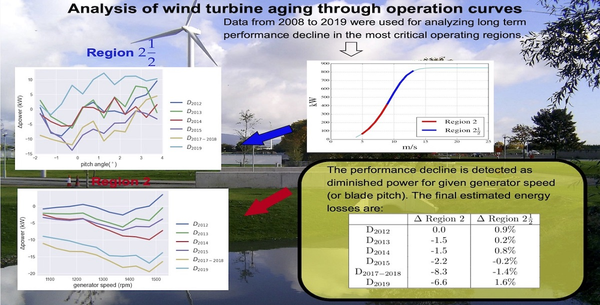
The worsening with age of technical systems performance is a matter of fact which is particularly timely to analyze for horizontal-axis wind turbines because they constitute a mature technology. On these grounds, the present study deals with the assessment of wind turbine performance decline with age. The selected test case is a Vestas V52 wind turbine, installed in 2005 at the Dundalk Institute of Technology campus in Ireland. Operation data from 2008 to 2019 have been used for this study. The general idea is analyzing the appropriate operation curves for each working region of the wind turbine: in Region 2 (wind speed between 5 and 9 m/s), the generator speed–power curve is studied, because the wind turbine operates at fixed pitch. In Region 2 $\raisebox{1ex}{$1$}\!\left/ \!\raisebox{-1ex}{$2$}\right.$ (wind speed between 9 and 13 m/s), the generator speed is rated and the pitch control is relevant: therefore, the pitch angle–power curve is analyzed. Using a support vector regression for the operation curves of interest, it is observed that in Region 2, a progressive degradation occurs as regards the power extracted for given generator speed, and after ten years (from 2008 to 2018), the average production has diminished of the order of 8%. In Region 2 $\raisebox{1ex}{$1$}\!\left/ \!\raisebox{-1ex}{$2$}\right.$, the performance decline with age is less regular and, after ten years of operation, the performance has diminished averagely of the 1.3%. The gearbox of the test case wind turbine was substituted with a brand new one at the end of 2018, and it results that the performance in Region 2 $\raisebox{1ex}{$1$}\!\left/ \!\raisebox{-1ex}{$2$}\right.$ has considerably improved after the gearbox replacement (+3% in 2019 with respect to 2018, +1.7% with respect to 2008), while in Region 2, an improvement is observed (+1.9% in 2019 with respect to 2018) which does not compensate the ten-year period decline (−6.5% in 2019 with respect to 2008). Therefore, the lesson is that for the test case wind turbine, the generator aging impacts remarkably on the power production in Region 2, while in Region 2 $\raisebox{1ex}{$1$}\!\left/ \!\raisebox{-1ex}{$2$}\right.$, the impact of the gearbox aging dominates over the generator aging; for this reason, wind turbine refurbishment or component replacement should be carefully considered on the grounds of the wind intensity distribution onsite.

1. Introduction

Horizontal-axis wind turbines constitute a mature technology; therefore, worldwide, there is a huge number of industrial wind farms that have been operating since approximately a couple of decades ago, which represents the end of their theoretical lifetime. Since it is well-known that performance decline with age substantially affects all the technical systems [1], it would therefore be possible to analyze in depth this issue with regard to wind turbines, especially in light of the widespread availability of Supervisory Control And Data Acquisition (SCADA) data. This objective has scientific interest as well as practical interest, and it is connected to the perspective of refurbishing and repowering wind turbines [2] that have been operating for a number of years.

Unexpectedly, the analysis of wind turbine aging is an overlooked topic in wind energy literature (many more studies are devoted to reliability analysis [3,4,5,6]) and few are the studies dealing with it. In [7], public data of actual and theoretical load factors of 282 wind farms sited in UK are analyzed; the methodology is substantially statistical and it is based on the regression (possibly adjusted on the resource trend and on site-specific information) of the load factors against the age. The main result of [7] is that wind turbines are estimated to lose $1.6\pm 0.2\%$ of their output per year, and this is equivalent to an increase of the 9% of the levelized cost of electricity in twenty years’ time. A similar approach is employed in [8]: a regression between the capacity factor and the age of wind turbines in Sweden is attempted; the yearly weather fluctuations are taken into account by including sine and cosine functions of the age in the regression. The estimate is that the lifetime (20 years) energy loss is of the order of 6%, considerably lower with respect to the results in [7].

The studies in [7,8] are a statistical analysis of yearly cumulative data of wind farms. Another line of research is possible as regards wind turbine aging, which consists in high-level operation data analysis: in fact, it is remarkable that several techniques have been developed and applied for wind turbine condition monitoring [9,10,11,12,13,14,15] and precision performance analysis [16,17,18,19,20,21,22], as is summarized for example in [23], but very few studies are devoted to the use of the same kind of techniques for the analysis of wind turbine aging. At present, two studies of this kind are available in the literature. In [24], the aging assessment is conducted by discussing what are the appropriate SCADA parameters to monitor and the analyzed targets are power fluctuations, vibrations and components heating. An interesting study, which constitutes the premise for the present work, is given in [25]: the test case is the same as in this study and it is a Vestas V52 wind turbine, installed in 2005 at the Dundalk Institute of Technology in Ireland. Operation data from 2008 up to 2019 have been analyzed in [25] and an overall wind turbine power and energy degradation in the order of 5% has been determined over the 13-year lifetime: the analysis has been based on a multivariate data-driven model whose target is the power of the wind turbine of interest. An important point of strength of the test case, and consequently of [25] and of the present study, is that in October 2018 the gearbox of the wind turbine reached its end of life and this component was substituted in July 2019: therefore, since July 2019, the wind turbine has been running with a new gearbox and the rest of the components aged fourteen years. This situation allowed estimating in [25], through appropriate operation data analysis, that the gearbox aging contributes approximately one third of the performance decline of the wind turbine.

Basing on the preliminary results in [25], the general idea of the present work is studying wind turbine aging through the analysis of appropriate operation curves. The simplest and most straightforward curve of a wind turbine is the power curve [26,27,28,29], because it connects directly the input (wind intensity) to the output (produced power). There are other instructive operation curves [30] of a wind turbine: examples can be the rotor speed–power curve, the generator speed–power curve, the blade pitch–power curve [31] and these curves have been mainly employed in the literature for condition monitoring purposes.

The approach of this study consists in analyzing separately the appropriate operation curves of the test case wind turbine for each region of the power curve (through the binning method, as recommended by the International Electrotechnical Commission IEC [32]): in particular, in Region 2 (wind intensity between 5 and 9 m/s), the wind turbine operates to extract maximum power, the blade pitch angle is set to approximately $0^{\circ }$ and the generator speed increases with the wind intensity. In this working region, the generator speed–power curve is selected as the operation curve of interest. In Region 2 $\raisebox{1ex}{$1$}\!\left/ \!\raisebox{-1ex}{$2$}\right.$ (wind intensity between 9 and 13 m/s), the generator speed is rated and the wind turbine regulates the pitch to control the power extraction: in this working region, the operation curve of interest is the blade pitch–power curve. By analyzing the evolution in time of these curves, it is possible to appreciate the different aging depending on the operation regime: in particular, distinct aging of the generator is observed in the fact that, as years pass by, less power is extracted for given generator speed. It should be noticed that this result is scientifically novel because, to the best of the authors’ knowledge, similar conclusions have not been obtained elsewhere in the literature and, furthermore, this result has relevant practical applications in the wind turbine management.

Another key point of this study is that the curves describing the wind turbine in its early functioning years (2008) can be modeled, and in this work, a support vector regression (SVR) with Gaussian kernel is selected: the loss of energy due to aging for each operation region can therefore be estimated quantitatively by comparing the measured curves against the curves that are simulated using the SVR model which is trained with the data in the early functioning of the wind turbine. In other words, the evolution in time of the performance of the wind turbine is encoded in how the residuals between measurements and model estimate change.

It is also important to recall that since July 2019 the wind turbine has been operating with a brand new gearbox, while all the other components are aged fourteen years: by comparing this data set against the oldest ones and against the one immediately before the gearbox replacement (2018), it is possible to argue that most of the recovered energy is concentrated in Region 2 $\raisebox{1ex}{$1$}\!\left/ \!\raisebox{-1ex}{$2$}\right.$ and that, as observed in [25], only one third approximately of the overall production level of the 2008 has been recovered. The analysis of the operation curves presented in this work allows interpreting this matter of fact: most of the production, which has not been recovered with the gearbox replacement, regards Region 2 and therefore it can be stated that in Region 2 the aging of the generator has been particularly impacting along fourteen years of wind turbine lifetime. On the other hand, in Region 2 $\raisebox{1ex}{$1$}\!\left/ \!\raisebox{-1ex}{$2$}\right.$ the impact of the gearbox aging dominates the generator aging because the performance of the wind turbine is more sensitive on the gearbox efficiency [33]), since the generator speed is rated and the mechanical solicitations are highest: in this working region, it is observed that the replacement of the gearbox restores the optimal performance. Substantially, the general lesson is that the profitability of the substitution of a component for an aged wind turbine depends on how much time the wind turbine, due to the on site wind intensity conditions, operates in each working region. These kind of considerations are particularly important when conceiving possible refurbishment interventions on aged wind turbines.

The structure of the manuscript is therefore the following: in Section 2, the test case wind turbine and the data sets at disposal for the present study are described; Section 3 is devoted to the methods; the results are collected and discussed in Section 4; conclusions are drawn and further directions of the present work are indicated in Section 5.

2. The Test Case and the Data Set

The test case is the same as in the previous study [25]: therefore, the present Section has substantial overlap with [25], but more information is added, which is related to the improved methodology developed in this work.

In October 2005, the Dundalk Institute of Technology installed a Vestas V52 wind turbine on its campus. The turbine has a hub height of 60 m and a rotor diameter of 52 m. The wind turbine, as shown in Figure 1 which is reported from [25], is located at a peri-urban coastal site [34]. The system is grid connected behind the main campus electricity meter and the produced electricity is primarily consumed onsite.

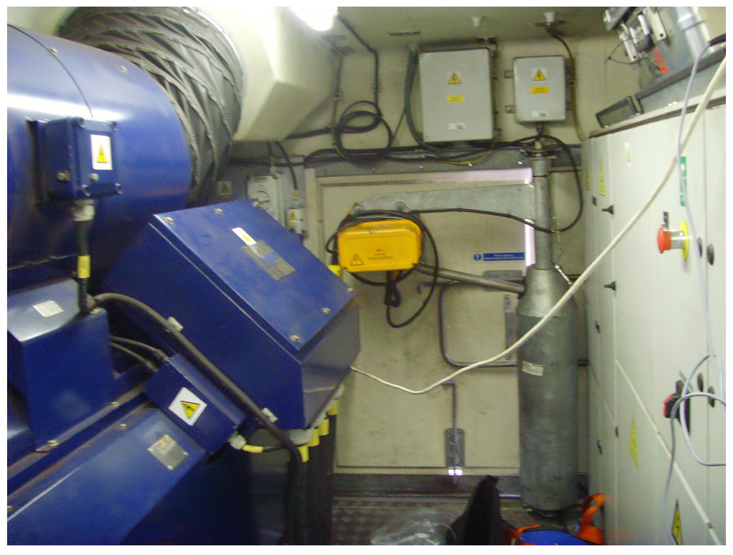
The Vestas V52 wind turbine has been widely installed worldwide in the past years: it is a semi-variable speed system with doubly fed induction generator (DFIG). The model of the generator in case is a Weier 850 kW, shown in Figure 2, and the main features are reported in

Table 1. Generator principal specifications.

Specification	Data
Model	DVSGF 400/4L SP
Rated Power	850 kW
Rated stator voltage	690 V
Rated stator frequency	50 Hz
No. of poles	4
Weight	3755 kg
Moment of inertia	35.7 kg${\mathrm{m}}^2$

. The wind turbine has an active pitching system: the blade pitch angles of all three rotor blades are controlled simultaneously by a hydraulic pitch control system using the Vestas Opti-tip^TM and Opti-speed^TM control mechanisms.

Time series data of a number of turbine parameters are logged by the wind turbine SCADA system in 10 min average values. The data available for the present study are indicated in

Table 2. Supervisory Control And Data Acquisition (SCADA) parameters analyzed.

Parameter	Units	Symbol
Wind Speed	(m/s)	v
Wind Speed Standard Deviation	(m/s)	${\delta }_v$
Wind Direction	(deg)	$\theta$
Ambient Temperature	(${}^{\circ }$C)	$T_{ext}$
Rotor Speed	(rpm)	$\omega$
Blade Pitch Angle	(deg)	$\beta$
Generator Speed	(rpm)	$\mathsf{\Omega }$
Power	(kW)	P
Gear oil Temperature	(${}^{\circ }$C)	$T_{oil}$

and have been organized in 12-months packets, except for the 2019 data set, which consists in six months of data.

The data sets are therefore indicated in the following as follows:

• ${\mathrm{D}}_{2008}$
• ${\mathrm{D}}_{2012}$
• ${\mathrm{D}}_{2013}$
• ${\mathrm{D}}_{2014}$
• ${\mathrm{D}}_{2015}$
• ${\mathrm{D}}_{2017-2018}$
• ${\mathrm{D}}_{2019}$ (6 months).

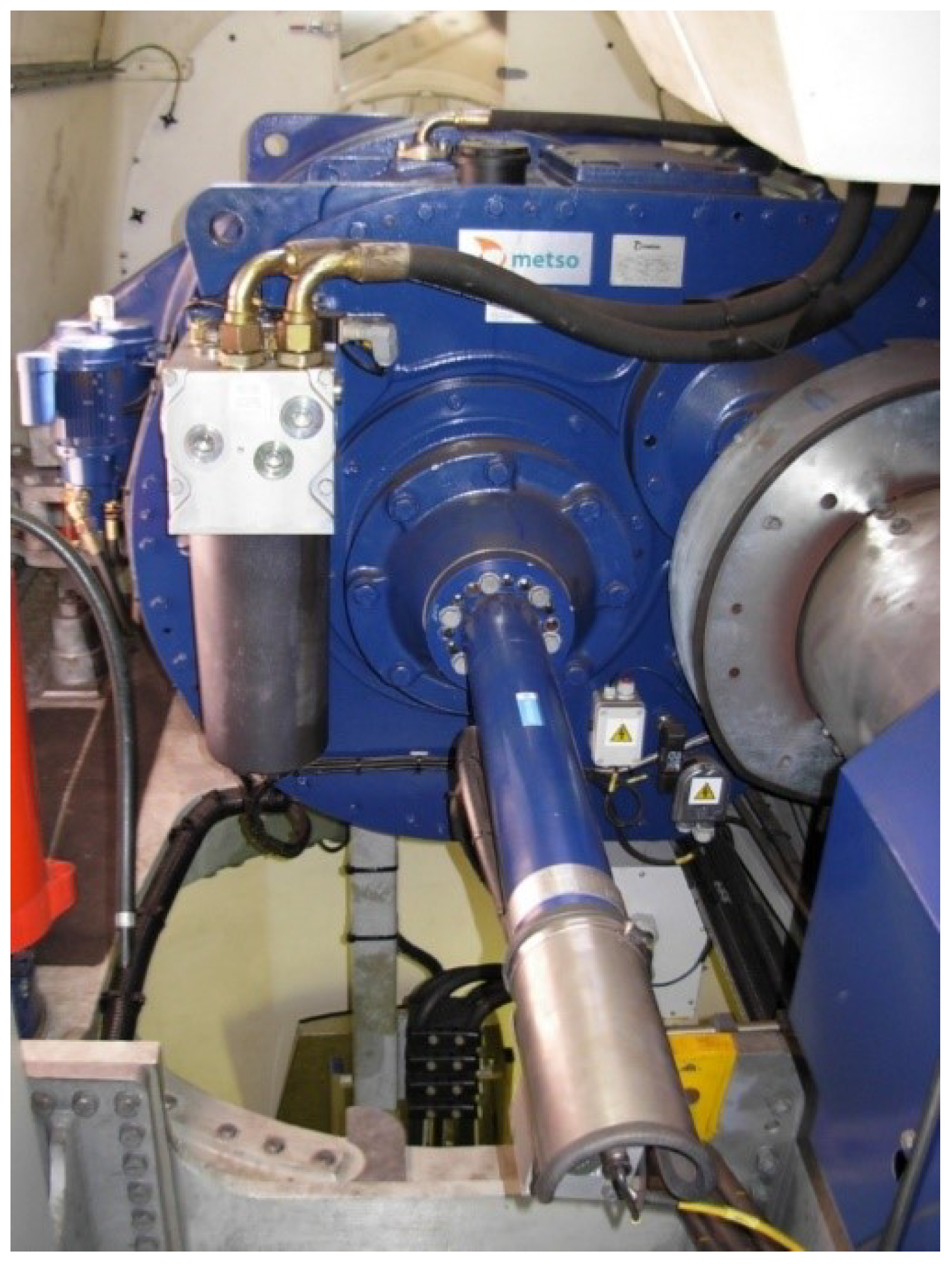
In October 2018, the wind turbine gearbox, shown in Figure 3 and principal specifications in

Table 3. Gearbox principal specifications; Reprint with permission [25]; 2020, MDPI.

Specification	Data
Model	PLH-400V52
Rated Power	935 kW
Rated RPM (Low speed shaft)	26 ${\min }^{-1}$
Gearing ratio	61.799
Weight	5400 kg

which are reported from [25], reached the end of life after thirteen years of operation and it was consequently replaced with a brand new gearbox of the same model and specifications in July 2019.

Therefore, referring to the data sets listed in Table 2, the six months of data recorded in 2019 describe the wind turbine operating with a completely new gearbox and with the rest of the components aged 14 years. This is an important point, because it is possible to compare the 2019 data set against the one immediately before the gearbox replacement (2017–2018) and against the one in the early days of wind turbine functioning (2008).

For each data set, data have been filtered on wind turbine normal operation by employing the appropriate time counter available in the SCADA logger. Subsequently, each data set has been divided according to the operation region, as indicated in

Table 4. Operation regions for the test case wind turbine.

Region	Condition
2	$5\le v\le 9$
2 $\raisebox{1ex}{$1$}\!\left/ \!\raisebox{-1ex}{$2$}\right.$	$9<v\le 13$

, on the grounds of nacelle wind intensity v. It should be noticed that in general, all the region between cut-in and rated wind speed is indicated as Region 2 but, in order to distinguish the working principles, also the notation of Table 4 can be adopted. Region 2 $\raisebox{1ex}{$1$}\!\left/ \!\raisebox{-1ex}{$2$}\right.$ and Region 2 are distinguished for the purposes of this study because the control works differently: in Region 2, the wind turbine operates at full load, the blade pitch is constant (set at a value approximately vanishing), and the generator speed increases with increasing wind intensity v; in Region 2 $\raisebox{1ex}{$1$}\!\left/ \!\raisebox{-1ex}{$2$}\right.$, the generator speed is rated and the wind turbine works in partial load which is controlled through the blade pitch angle.

A detailed analysis of the onsite climatology is out of the scope of the present work; nevertheless an important information for understanding the net aging energy balance along all the power curve from cut-in to rated regards the fact that, during a year, the wind turbine operates in Region 2 approximately three times more time than in Region 2 $\raisebox{1ex}{$1$}\!\left/ \!\raisebox{-1ex}{$2$}\right.$. Therefore, the aging trend is substantially dominated by Region 2.

3. The Method

3.1. Operation Curve Analysis

The power of a wind turbine, below rated speed, is defined as in Equation (1) [25]:

$$P=\frac{1}{2}\rho A{C}_p\left(\lambda ,\beta \right)v^3,$$

(1)

where v is the undisturbed wind speed, $\rho$ is the air density, A is the area swept by the rotor, $C_p$ is the power factor which is function of the tip speed ratio $\lambda$ and of the blade pitch angle $\beta$. The power factor $C_p$ is a nonlinear function of $\lambda$ and $\beta$.

The simplest operation curve is the power curve: the International Electrotechnical Commission (IEC) has recommended the binning method for analyzing it [32]. It consists in grouping power data in wind speed bins of 0.5 or 1 m/s amplitude, as applied also in [25].

Given the i-th wind speed bin, the average wind speed for the bin is computed as in Equation (2):

$${\overline{v}}_i=\frac{1}{N_i}\sum _{j=1}^{N_i}{v}_{i,j}$$

(2)

and the average power for the bin is computed as in Equation (3):

$${\overline{P}}_i=\frac{1}{N_i}\sum _{j=1}^{N_i}{P}_{i,j}$$

(3)

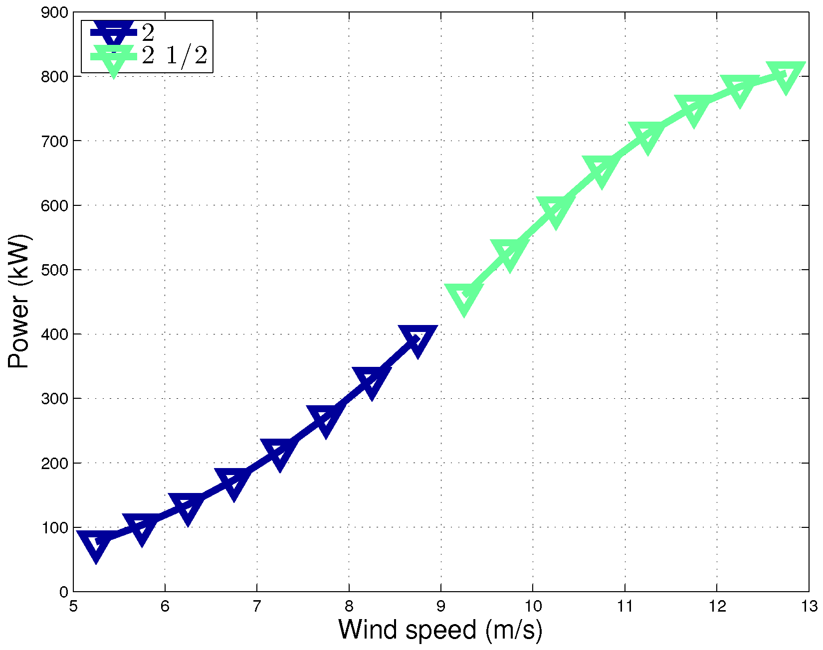
where $v_{i,j}$ is the normalized measured wind speed of the j-th data set in the i-th wind speed bin, $P_{i,j}$ is the normalized measured power output of the j-th data set in the i-th wind speed bin and $N_i$ is the population of the i-th wind speed bin. An example of power curve from cut-in to rated is reported in Figure 4, where the Regions 2 and 2 $\raisebox{1ex}{$1$}\!\left/ \!\raisebox{-1ex}{$2$}\right.$ are distinguished.

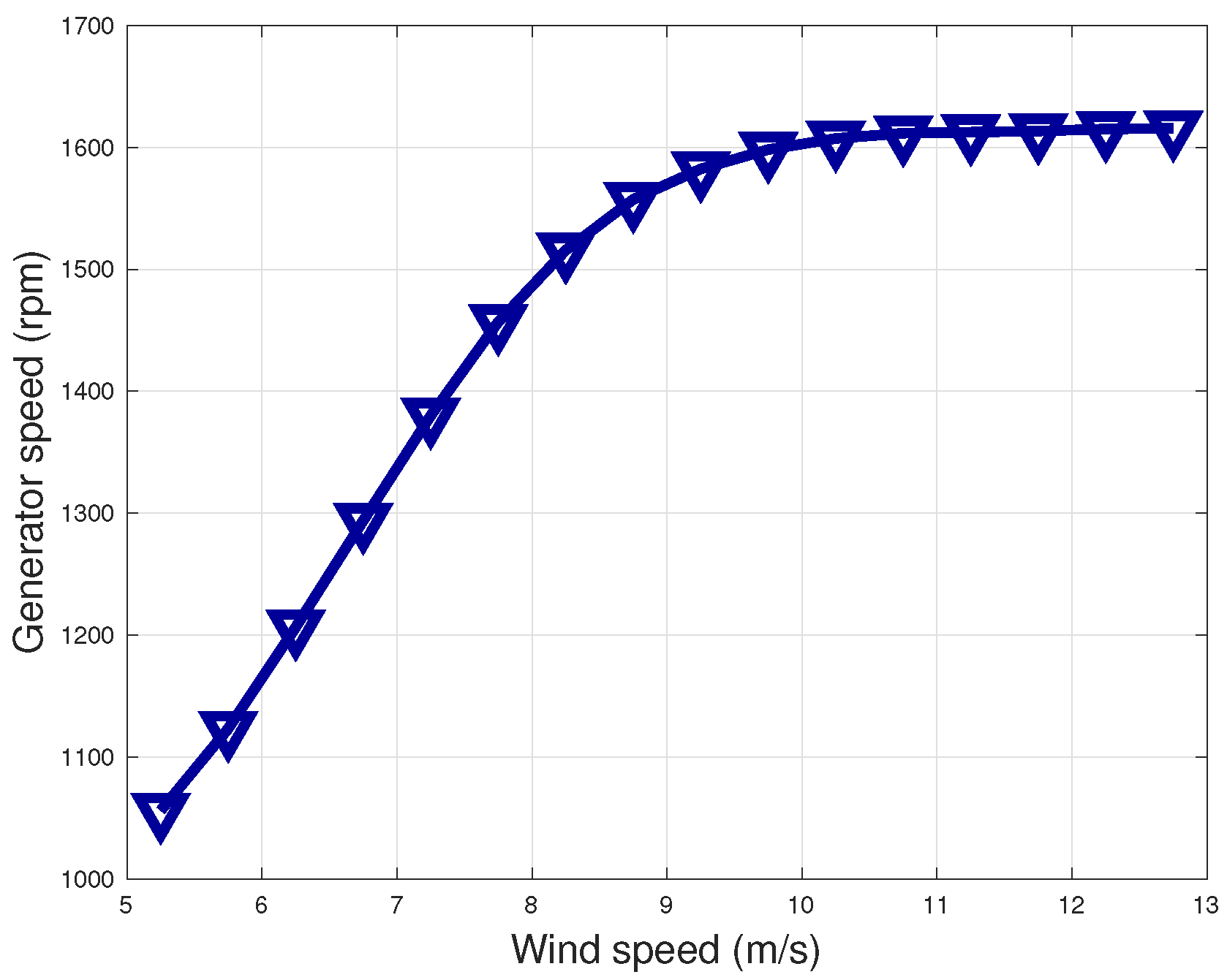
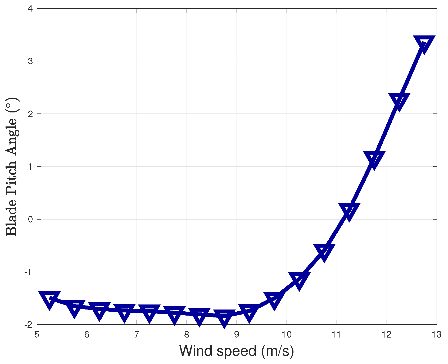
Other sample operation curves are reported in Figure 5 and Figure 6 for the data set ${\mathrm{D}}_{2008}$: they are respectively the binned wind speed–generator speed curve and the binned wind speed–blade pitch angle curve. Figure 5 and Figure 6 are reported because from their visualization it is possible to distinguish Region 2 from Region 2 $\raisebox{1ex}{$1$}\!\left/ \!\raisebox{-1ex}{$2$}\right.$: the generator speed increases practically linearly (Region 2) and saturates at $v\simeq 9$ m/s (Region 2 $\raisebox{1ex}{$1$}\!\left/ \!\raisebox{-1ex}{$2$}\right.$ begins); conversely, the blade pitch angle is practically constant up to $v\simeq 9$ m/s (Region 2) and then increases (Region 2 $\raisebox{1ex}{$1$}\!\left/ \!\raisebox{-1ex}{$2$}\right.$).

For the prosecution of this study, it is important to notice that other operation curves can be of interest and one can put in abscissa and in ordinate whatever couple of operation variables $(G_1,G_2)$. In general, there are good reasons for avoiding to put in abscissa the wind speed: they deal with the fact that commonly wind turbines measure the wind flow behind the rotor and the undisturbed wind speed is reconstructed through a nacelle transfer function. In other words, there can be data quality issues as regards the nacelle wind speed measurements [35,36] and it can be convenient to analyze operation curves where abscissa and ordinate are working parameters of the wind turbine.

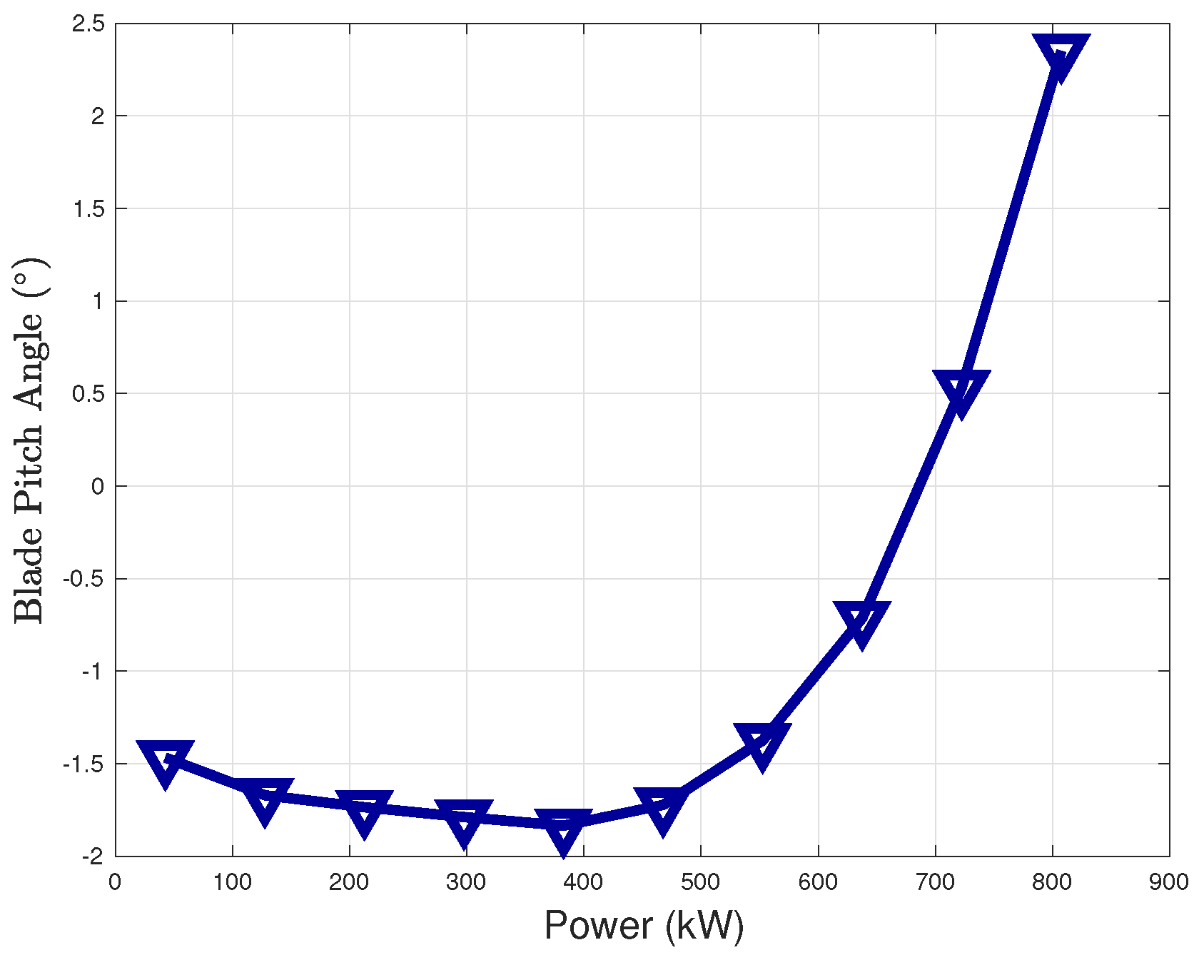
For a generic selection $(G_1,G_2)$, the Equations remain (2) and (3), with v substituted by $G_1$ and P substituted by $G_2$: it is important to select meaningful bins for the $G_1$ operation variable, on the grounds of the range that it can assume. For example, in Figure 7 and Figure 8, examples of binned power-generator speed and power-blade pitch angle curves are reported: in this case $G_1$ is the power P and the data are averaged in bins whose amplitude is the 10% of the rated power.

For the objectives of the present study, it is more interesting to separate Region 2 from Region 2 $\raisebox{1ex}{$1$}\!\left/ \!\raisebox{-1ex}{$2$}\right.$ and analyze in depth the operation curves associated to variables which are not saturated or constant for the given Region. The summary of the curves of interest for each working Region is reported in

Table 5. Analyzed operation curves and working range of the variables.

Region	Curve	$({\mathit{G}}_1,{\mathit{G}}_2)$	${\mathit{G}}_1$ Range	${\mathit{G}}_1$ bin
2	Power curve	$(v,P)$	[5, 9] m/s	0.5 m/s
2	Generator speed–power curve	$(\mathsf{\Omega },P)$	[1050, 1550] rpm	50 rpm
2 1/2	Power curve	$(v,P)$	[9, 13] m/s	0.5 m/s
2 1/2	Blade pitch angle–power curve	$(\beta ,P)$	$[-2^{\circ },4^{\circ }]$	${0.5}^{\circ }$

.

It should be mentioned that recent developments in the wind energy literature have been achieved as regards the comprehension of the performance worsening due to blade degradation [37]. At present, the available studies are mainly numerical simulations but, for completeness in this work, the wind speed–rotor speed curve has been preliminarily analyzed, in order to inquire if the amount of torque extracted for given wind intensity visibly degrades with age of the wind turbine: no relevant degradation has been observed and therefore the analyzed operation curves are those listed in Table 5.

3.2. Support Vector Regression

The objective of this part of the work is modeling the curves indicated in Table 5 through a data-driven regression. The rationale for this is a quantitative analysis of the production decline with age. This can be achieved by training a data-driven regression for the curves in Table 5, because for each of those curves the target is the power P. The procedure is as follows: using the data set describing the wind turbine in its early operation era (namely ${\mathrm{D}}_{2008}$), the regression is trained; the so-established models are subsequently used for simulating the output (i.e., the power P) for all the data sets posterior to ${\mathrm{D}}_{2008}$; finally the residuals between the measurements and the simulated powers are analyzed. If the performance of the wind turbine declines with age, the powers which have been simulated using ${\mathrm{D}}_{2008}$ as training data set will be systematically higher than the measurements, in a manner which is expected to increase in time.

In the following, these concepts are systematized. The regression type which has been selected for this study is a support vector regression with Gaussian kernel [38]: this kind of regression has been used in the literature [39,40] for wind turbine performance monitoring and has proven to be effective for tackling the nonlinear dependence of the power on ambient conditions and working parameters. Actually, in general the operation curves of a wind turbine are nonlinear (compare against Figure 4, Figure 5, Figure 6, Figure 7 and Figure 8) and therefore a nonlinear regression (as the one selected in this study) is required. It is the same type of regression which has been adopted in [25] and therefore the explanation of the general methodology has overlaps with that manuscript (Equations (4)–(13)): nevertheless, the application is different with respect to [25] because different operation curves are considered.

Consider at first a linear model (Equation (4)):

$$f\left(\mathit{X}\right)=\mathit{X}\mathbf{\beta }+\mathit{b},$$

(4)

where $\mathit{X}$ is the matrix of input variables (the covariates are grouped according to the columns, the observations are grouped according to the rows), $\mathbf{\beta }$ is the vector of regression coefficients and $\mathit{b}$ is the intercept vector. The objective of the selected regression type is finding $f\left(\mathit{X}\right)$ with the minimum norm value ${\mathbf{\beta }}^{\prime }\mathbf{\beta }$ subject to the residuals between the measurement Y and the model estimate $f\left(\mathit{X}\right)$ being lower than a threshold $ϵ$ for each n-th observation (Equation (14)):

$$\left|Y_n-{\mathit{X}}_n\mathbf{\beta }+b_n\right|\le ϵ$$

(5)

The optimization of the model consists in a trade-off between the flatness of $f\left(\mathit{X}\right)$ and the amount up to which residuals higher than $ϵ$ are tolerated. This optimization problem is typically rephrased through the Lagrange dual formulation: the function to minimize is $L\left(\alpha \right)$ (Equation (6)):

$$L\left(\alpha \right)=\frac{1}{2}\sum _{i=1}^N\sum _{j=1}^N\left({\alpha }_i-{\alpha }_i^{*}\right)\left({\alpha }_j-{\alpha }_j^{*}\right){\mathit{X}}_i^{\prime }{\mathit{X}}_j+ϵ\sum _{i=1}^N\left({\alpha }_i+{\alpha }_i^{*}\right)+\sum _{i=1}^N{Y}_i\left({\alpha }_i^{*}-{\alpha }_i\right),$$

(6)

with the constraints (Equation (7))

$$\begin{array}{c}\hfill \sum _{n=1}^N\left({\alpha }_n-{\alpha }_n^{*}\right)=0\\ \hfill 0\le {\alpha }_n\le C\\ \hfill 0\le {\alpha }_n^{*}\le C,\end{array}$$

(7)

where C is the box constraint.

The $\mathbf{\beta }$ parameters are given in Equation (8):

$$\mathbf{\beta }=\sum _{n=1}^N\left({\alpha }_n-{\alpha }_n^{*}\right){\mathit{X}}_n.$$

(8)

If either ${\alpha }_n$ or ${\alpha }_n^{*}$ is non-vanishing, the corresponding observation is called a support vector.

Once the model has been trained by computing the $\mathbf{\beta }$ coefficients, it can be used for predicting new values, given the input variables matrix, through the function (Equation (9)):

$$f\left(\mathit{X}\right)=\sum _{n=1}^N\left({\alpha }_n-{\alpha }_n^{*}\right){\mathit{X}}_n^{\prime }\mathit{X}+\mathit{b}.$$

(9)

A nonlinear support vector regression is obtained by replacing in the above formulas the dot products between the observations matrix with a nonlinear kernel function (Equation (10)):

$$G\left({\mathit{X}}_1,{\mathit{X}}_2\right)=\langle \phi \left({\mathit{X}}_1\right)\phi \left({\mathit{X}}_2\right)\rangle ,$$

(10)

where $\phi$ is a transformation mapping the $\mathit{X}$ observations into the feature space.

A Gaussian kernel selection is given in Equation (11):

$$G\left({\mathit{X}}_i,{\mathit{X}}_j\right)=e^{-{∥{\mathit{X}}_i-{\mathit{X}}_j∥}^2}.$$

(11)

Then, for the nonlinear case, Equation (6) rewrites as in Equation (12):

$$L\left(\alpha \right)=\frac{1}{2}\sum _{i=1}^N\sum _{j=1}^N\left({\alpha }_i-{\alpha }_i^{*}\right)\left({\alpha }_j-{\alpha }_j^{*}\right)G\left({\mathit{X}}_i,{\mathit{X}}_j\right)+ϵ\sum _{i=1}^N\left({\alpha }_i+{\alpha }_i^{*}\right)+\sum _{i=1}^N{Y}_i\left({\alpha }_i^{*}-{\alpha }_i\right),$$

(12)

and Equation (9) for predicting rewrites as in Equation (13):

$$f\left(\mathit{X}\right)=\sum _{n=1}^N\left({\alpha }_n-{\alpha }_n^{*}\right)G\left({\mathit{X}}_n,\mathit{X}\right)+\mathit{b}.$$

(13)

The data sets are employed as follows for the regression:

• The training data set is randomly divided in two subsets: D0 (a random selection of $\frac{2}{3}$ of the data set) and D1 (the remainder $\frac{1}{3}$ of the data set). D0 is used for training the regression, D1 is used for setting the standards of the residuals between model estimates and measurements.
• A validation data set D2 is employed to quantify the performance deviation with respect to D1, through the analysis of the residuals between model estimates and measurements.

Consider Equation (14) with $i=1,2$.

$$R\left({\mathit{X}}_i\right)=Y\left({\mathit{X}}_i\right)-f\left({\mathit{X}}_i\right).$$

(14)

For $i=1,2$, one computes (Equation (15))

$${\mathsf{\Delta }}_i=100\frac{{\sum }_{\mathit{X}\in Dat{a}_i}\left(Y\left(\mathit{X}\right)-f\left(\mathit{X}\right)\right)}{{\sum }_{\mathit{X}\in Dat{a}_i}Y\left(\mathit{X}\right)}$$

(15)

and the quantity in Equation (16)

$$\mathsf{\Delta }={\mathsf{\Delta }}_2-{\mathsf{\Delta }}_1$$

(16)

provides an estimate of the performance deviation from data set D1 to D2 [16,20].

Substantially, the idea is that the model is trained on a data set (D0) and, for each target data set of interest (D2), the model is used for simulating the output on two data sets: the former (D1) belongs to the same period from which D0 is extracted and serves for standard setting as regards the residuals (Equation (14)). If the performance during the target data set D2 has changed (worsened or improved), the residuals should have different properties with respect to what happens in D1: referring to the case of interest regarding the aging decline, it is expected that for D2 the simulated data should be systematically higher than the measured ones and therefore the set $R\left({\mathit{X}}_2\right)$ should be distinguishable with respect to $R\left({\mathit{X}}_1\right)$.

The most straightforward data selection is extracting D0 and D1 from ${\mathrm{D}}_{2008}$ and selecting D2, once at a time, as each other yearly packet at disposal: this selection allows setting the standards using the data describing the wind turbine at its earliest functioning and analyzing how the performance evolves in time. The results are collected in Section 4. The peculiarity of the test case at disposal, regarding the substitution of the gearbox in October 2018, suggests another meaningful selection which will be explored as well in Section 4: extracting D0 and D1 from the data set immediately before the gearbox replacement (${\mathrm{D}}_{2017–2018}$) and selecting D2 as the post-replacement data set (${\mathrm{D}}_{2019}$). This latter selection allows to analyze clearly how the performance have changed in light of the intervention on the wind turbine.

In

Table 6. Structure of the SVR regressions for each operation region.

Region	Input	Output
2	Generator speed $\mathsf{\Omega }$	Power P
2 $\raisebox{1ex}{$1$}\!\left/ \!\raisebox{-1ex}{$2$}\right.$	Blade pitch angle $\beta$	Power P

, the set up of the models for each operation region is indicated: notice that, if one considers all the power curve span from cut-in to rated, each of the regressors in Table 6 would be insufficient for a reliable model for the power P, which should preferably be multivariate [41]. Having separated the operation regions, it is instead possible to keep the simplest structure for the regression, resembling the two-dimensional operation curves of interest.

4. Results

4.1. Operation Curve Analysis

4.1.1. Region 2

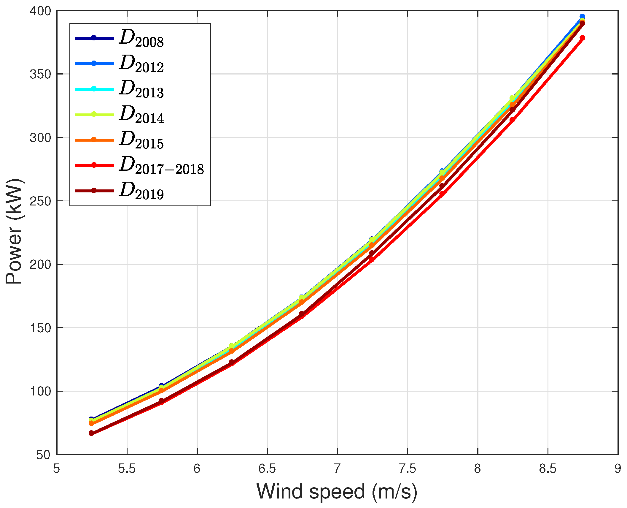
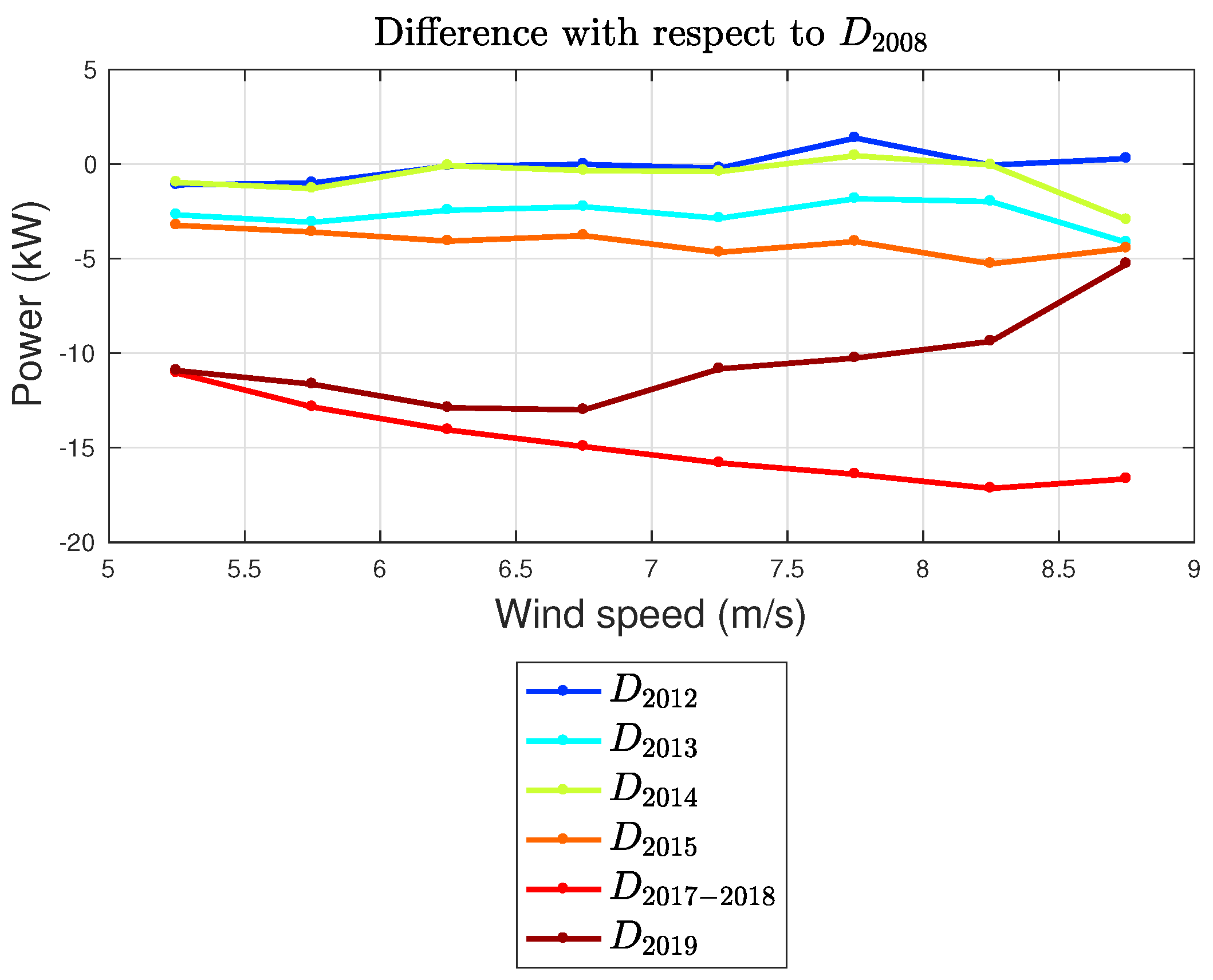
In Figure 9, the binned power curves in Region 2 for all the data sets at disposal are reported. For readability sake, Figure 10 reports the same kind of plot where, for each data set posterior to ${\mathrm{D}}_{2008}$, the difference of the binned power curve with respect to the one of ${\mathrm{D}}_{2008}$ is plotted. From Figure 10, it basically arises that the measured power curves in Region 2 after ${\mathrm{D}}_{2008}$ are always lower than in ${\mathrm{D}}_{2008}$. From ${\mathrm{D}}_{2015}$, the decrease becomes a little more evident and it exacerbates in ${\mathrm{D}}_{2017-2018}$: in ${\mathrm{D}}_{2019}$, the performance is still sensibly lower than ${\mathrm{D}}_{2008}$ but a little recovery with respect to ${\mathrm{D}}_{2017-2018}$ can be observed.

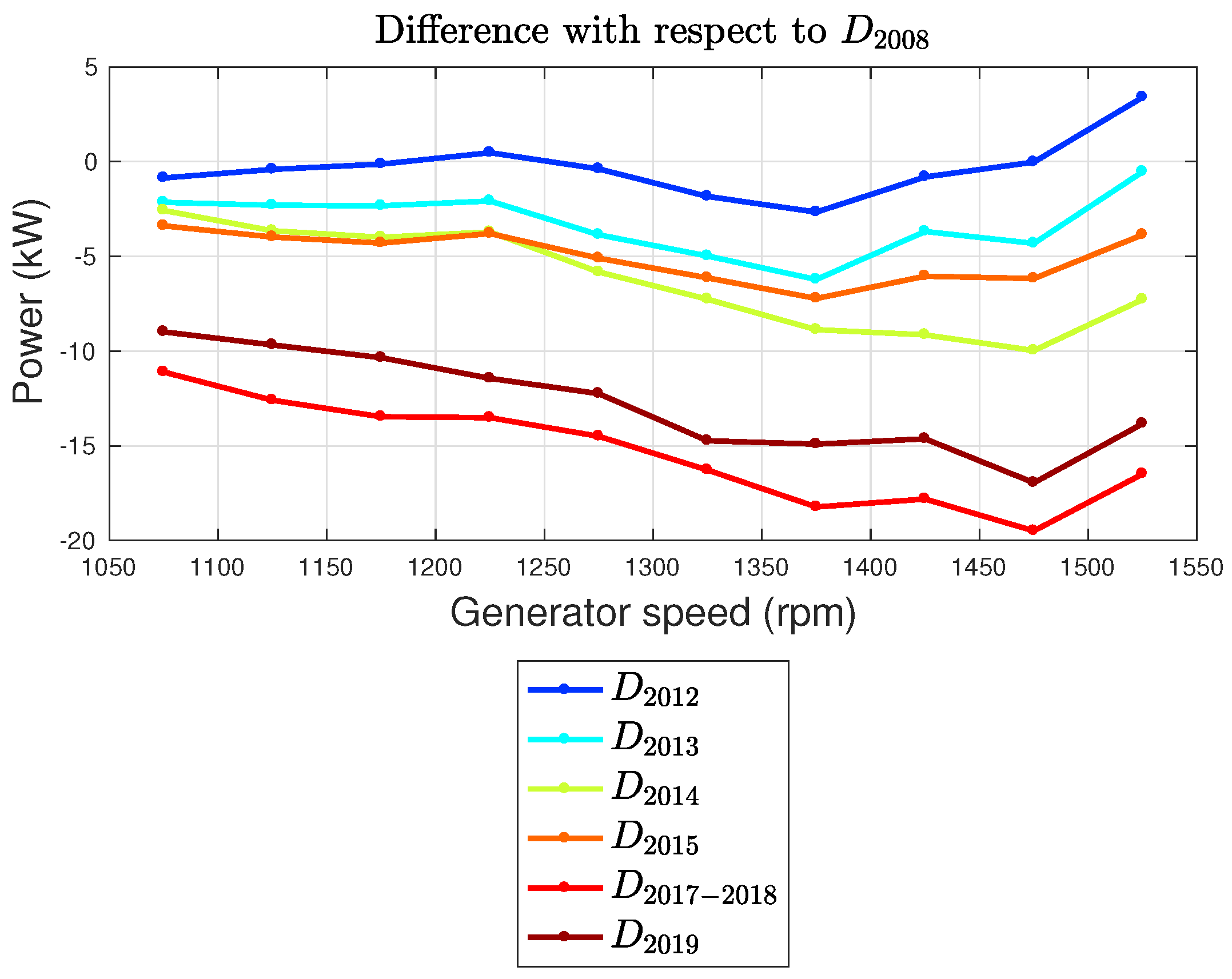
A similar situation occurs as regards Figure 11 and Figure 12, where the binned generator speed–power curves for Region 2 are reported. From these Figures, it arises that there is a progressive degradation of the amount of power extracted for given generator speed (which exacerbates after ten years of operation) and this could likely be interpreted as due to the generator aging. Consistently, after the replacement of the gearbox (${\mathrm{D}}_{2019}$), there is only a small performance recovery that could be interpreted as due to diminished vibrations in the drive-train, which may have reduced bearing heating in the drive shaft of the generator. Figure 11 and Figure 12 therefore indicate that the aging of wind turbines generator must be considered with attention when estimating the performance degradation in time.

4.1.2. Region 2 $\raisebox{1ex}{$1$}\!\left/ \!\raisebox{-1ex}{$2$}\right.$

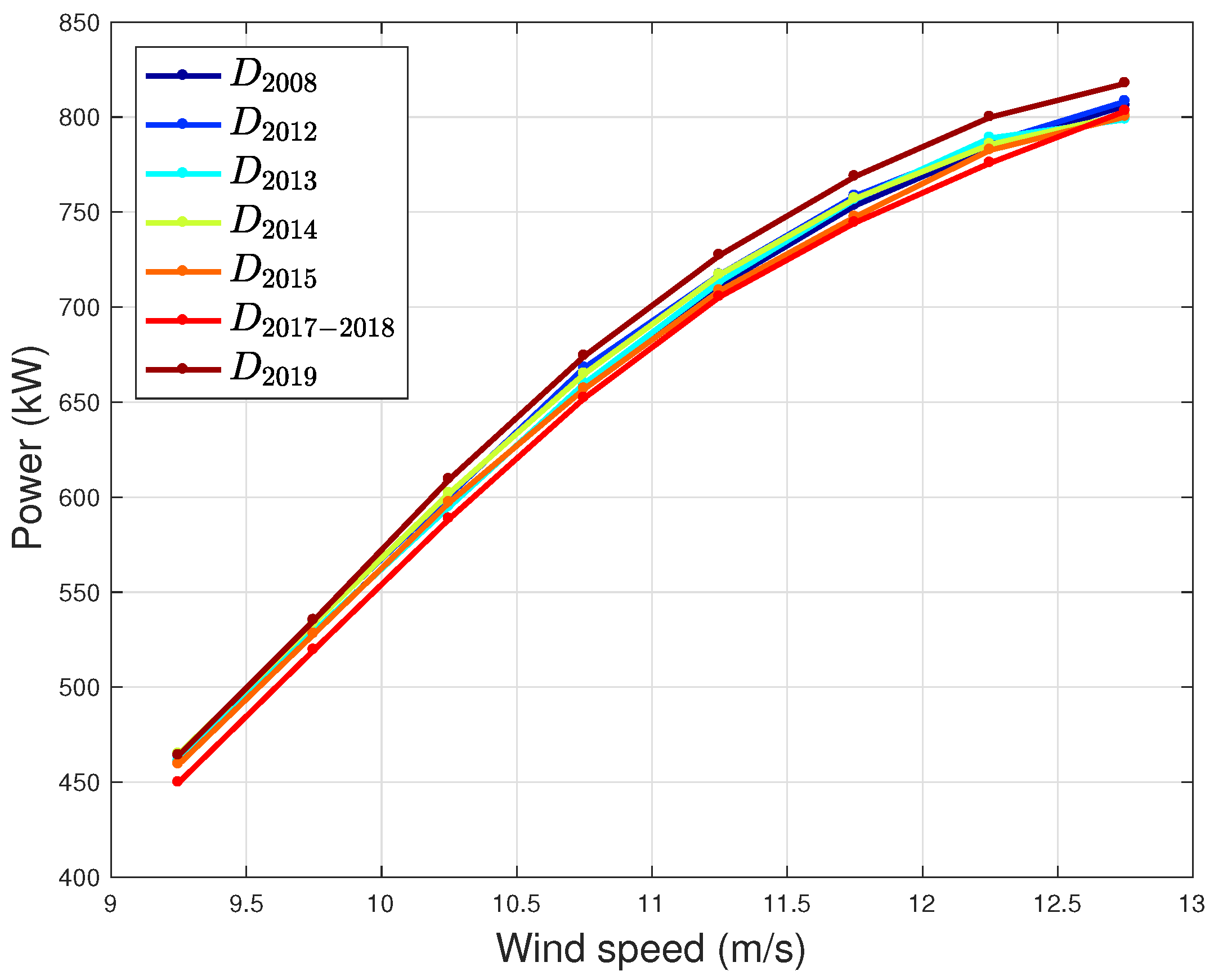
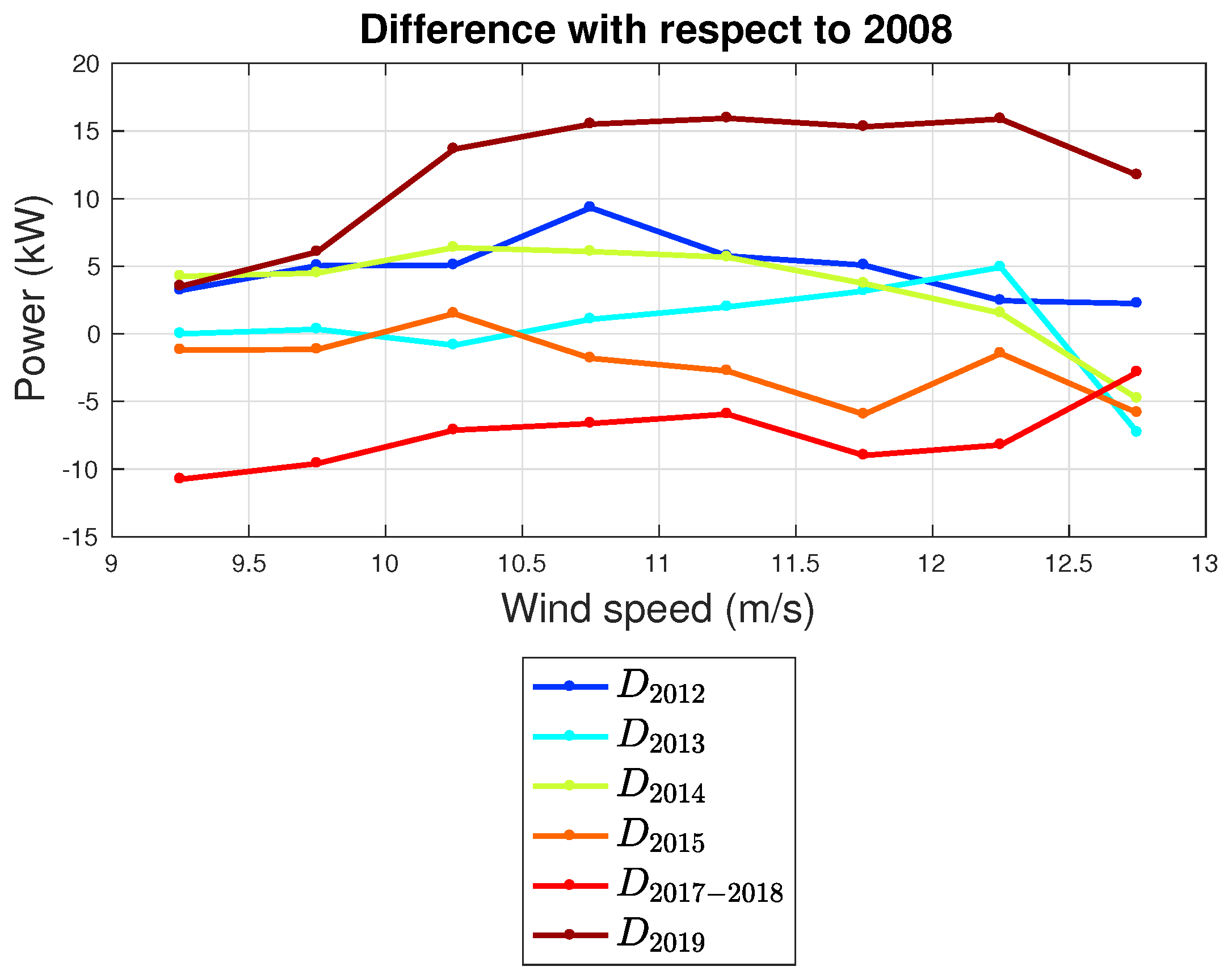
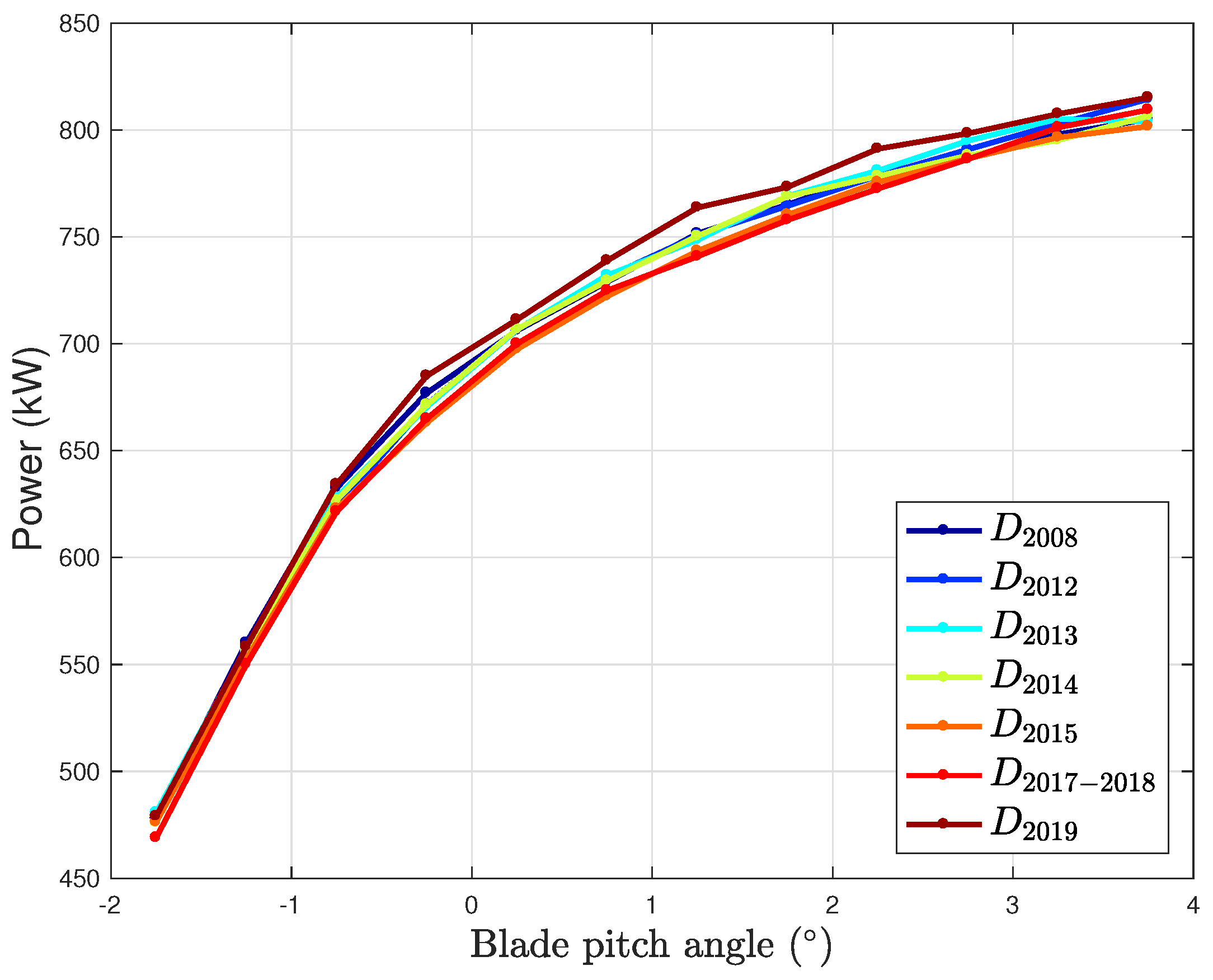
Figure 13 and Figure 14 report for Region 2 $\raisebox{1ex}{$1$}\!\left/ \!\raisebox{-1ex}{$2$}\right.$ the binned power curves and the difference with respect to ${\mathrm{D}}_{2008}$ of the binned power curve measured after ${\mathrm{D}}_{2008}$. It arises that before ${\mathrm{D}}_{2015}$, the measured power curves are substantially comparable to the reference in ${\mathrm{D}}_{2008}$, while with ${\mathrm{D}}_{2015}$ and more severely with ${\mathrm{D}}_{2017-2018}$ a clear performance degradation occurs. The performance in ${\mathrm{D}}_{2019}$ (therefore, after gearbox replacement) results being even higher than in the reference data set ${\mathrm{D}}_{2008}$. The lesson from Figure 9, Figure 10, Figure 11, Figure 12, Figure 13 and Figure 14 is that the aging of the generator seems to be more impacting in Region 2, while the aging of the gearbox is more important in Region 2 $\raisebox{1ex}{$1$}\!\left/ \!\raisebox{-1ex}{$2$}\right.$ and, consequently, after the gearbox replacement, substantially the standard level of performance has been restored in Region 2 $\raisebox{1ex}{$1$}\!\left/ \!\raisebox{-1ex}{$2$}\right.$, while it has not in Region 2. Figure 15 and Figure 16 represent the binned blade pitch angle–power curves and the difference of these curves with respect to ${\mathrm{D}}_{2008}$: these Figures corroborate the interpretation given by Figure 13 and Figure 14.

4.2. Support Vector Regression

4.2.1. Region 2

In

Table 7. Estimates of the average performance degradation in Region 2, with respect to ${\mathrm{D}}_{2008}$.

D2	$\mathsf{\Delta }$
${\mathrm{D}}_{2012}$	0.0%
${\mathrm{D}}_{2013}$	−1.5%
${\mathrm{D}}_{2014}$	−1.5%
${\mathrm{D}}_{2015}$	−2.2%
${\mathrm{D}}_{2017-2018}$	−8.3%
${\mathrm{D}}_{2019}$	−6.6%

, the results are reported for the average energy yield difference in Region 2 with respect to the D1 data set (which has been extracted from ${\mathrm{D}}_{2008}$), according to Equations (14)–(16). From Table 7, it arises that in ${\mathrm{D}}_{2012}$ the performance is averagely equal to ${\mathrm{D}}_{2008}$, while from ${\mathrm{D}}_{2013}$ an average decrease of the order of 1.5% occurs and it worsens to 2.2% in ${\mathrm{D}}_{2015}$ and, more severely, 8.3% in ${\mathrm{D}}_{2017-2018}$. The main result from Table 7 is therefore that along ten years in Region 2 a performance decline of the order of 8% is reached and this amount is remarkable. After the gearbox replacement (${\mathrm{D}}_{2019}$), the average performance is 6.6% lower than in ${\mathrm{D}}_{2008}$: this result indicates that the performance decline with age in Region 2 is mainly due to the aging of the generator and the replacement of the gearbox provides only a very partial recovery of the performance. These results expand and provide a substantial explanation to the findings of [25] dealing with the same test case: actually, in [25], a similar methodology has been applied to the whole power curve from cut-in to rated and an average performance decrease of the order of 5% is individuated in years 2017–2018 with respect to 2008. The results In Table 7 indicate that average behavior is actually driven mainly by the generator aging in Region 2.

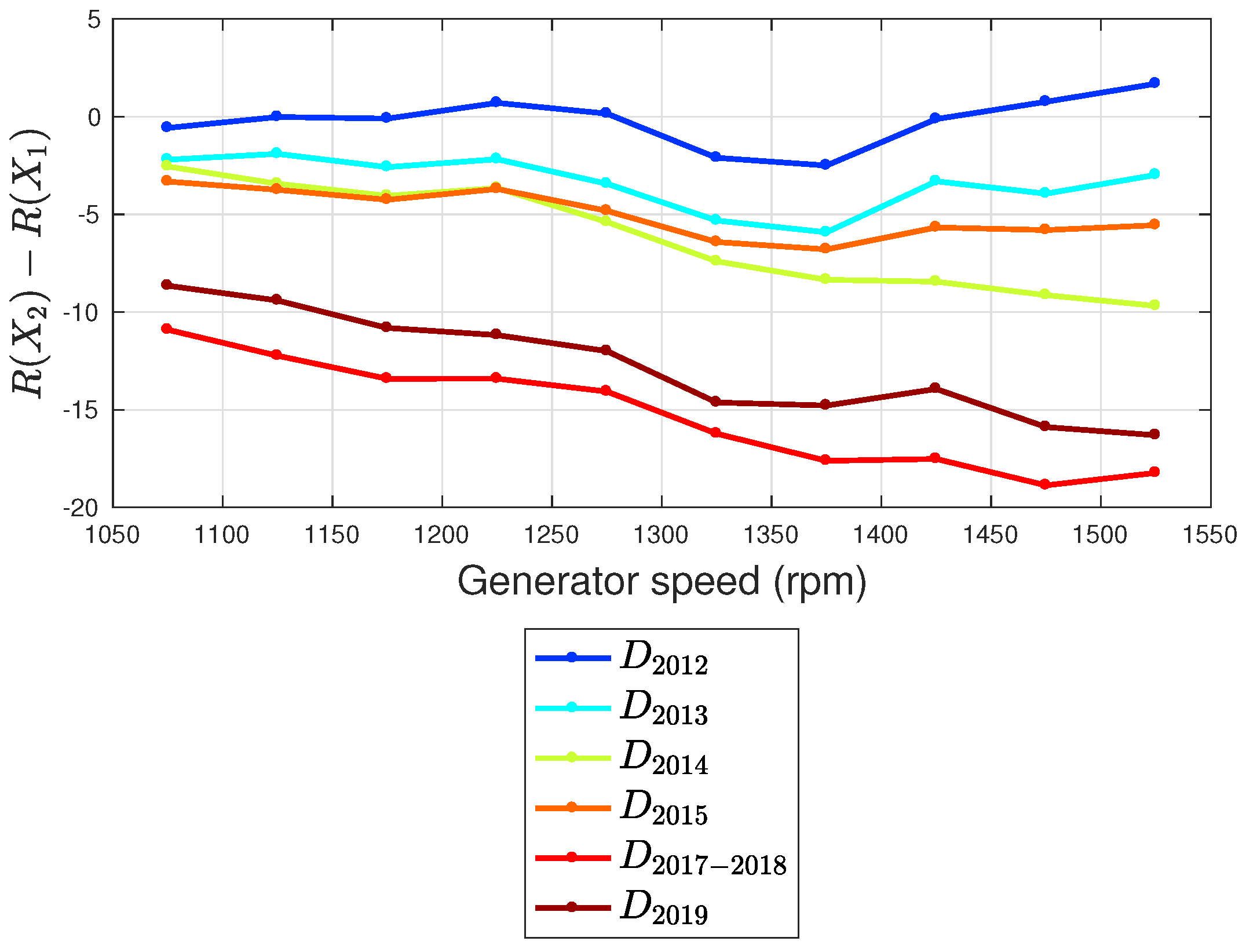
The results in Table 7 can be visualized in Figure 17: in Figure 17, the difference between the average curves of the residuals for data sets D1 and D2 is reported as a function of the generator speed (i.e., the input of the regression). It arises that the trends in Figure 17 fairly resemble those in Figure 12 and this confirms the consistency of the method.

The comparison between the data set immediately before (${\mathrm{D}}_{2017-2018}$) and immediately after (${\mathrm{D}}_{2019}$) the gearbox replacement can be performed by extracting D0 and D1 from ${\mathrm{D}}_{2017-2018}$ and D2 from ${\mathrm{D}}_{2019}$. It arises that, on average, after the gearbox replacement the wind turbine has produced in Region 2 the $\mathsf{\Delta }=1.9\%$ more than it would have done if the gearbox had not been replaced.

4.2.2. Region 2 $\raisebox{1ex}{$1$}\!\left/ \!\raisebox{-1ex}{$2$}\right.$

In

Table 8. Estimates of the average performance degradation in Region 2 $\raisebox{1ex}{$1$}\!\left/ \!\raisebox{-1ex}{$2$}\right.$, with respect to ${\mathrm{D}}_{2008}$.

D2	$\mathsf{\Delta }$
${\mathrm{D}}_{2012}$	0.9%
${\mathrm{D}}_{2013}$	0.2%
${\mathrm{D}}_{2014}$	0.8%
${\mathrm{D}}_{2015}$	−0.2%
${\mathrm{D}}_{2017-2018}$	−1.4%
${\mathrm{D}}_{2019}$	1.6%

, the results are reported for the average energy yield difference in Region 2 $\raisebox{1ex}{$1$}\!\left/ \!\raisebox{-1ex}{$2$}\right.$ with respect to the D1 data set (which has been extracted from ${\mathrm{D}}_{2008}$), according to Equations (14)–(16). From Table 8, it arises that up to ${\mathrm{D}}_{2014}$ the performance is in average slightly higher than in ${\mathrm{D}}_{2008}$, while from ${\mathrm{D}}_{2015}$ the trend inverts and an average decrease of the 1.5% is reached in ${\mathrm{D}}_{2017-2018}$. This result can be put in relation with those in Section 4.1.1 and those collected in Table 3 in [25]. From 2012 to 2014, the average performance decline along all the power curve is estimated [25] being less than 1%: this can be interpreted as the net effect of the performance comparable to the optimal in Region 2 $\raisebox{1ex}{$1$}\!\left/ \!\raisebox{-1ex}{$2$}\right.$ and the declining performance in Region 2 (Table 7) due to the generator aging. In [25] it has been estimated that in average ${\mathrm{D}}_{2017-2018}$ deviates with respect to ${\mathrm{D}}_{2008}$ of the order of the 5% along all the power curve below rated speed. On the grounds of the results in Table 7 and Table 8, it can be stated that this remarkable performance worsening which is visible after ten years of operation is due mainly to the generator aging and the gearbox too has given a contribution (differently with respect to the previous years of operation). It should be pointed out that the precise amount of the actual energy yield decline depends on how much time the wind turbine operates in Region 2 and how much in Region $\raisebox{1ex}{$1$}\!\left/ \!\raisebox{-1ex}{$2$}\right.$ and this in the end depends on the onsite climatology. In particular, a sensible average energy yield decline is visible in the present site because it is characterized by most frequent wind intensity occurrence in Region 2 (as indicated in Section 2).

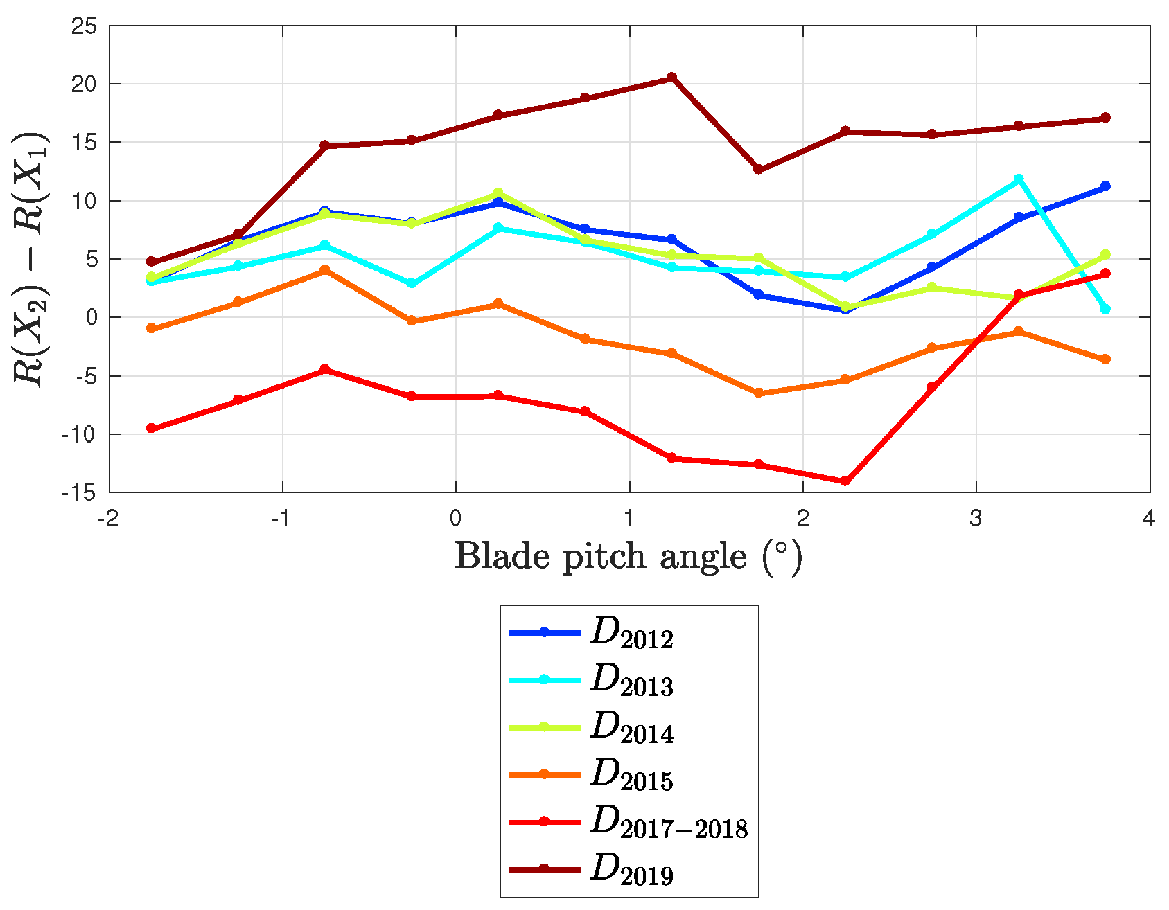
After the gearbox replacement (${\mathrm{D}}_{2019}$), the average performance is 1.6% higher than in ${\mathrm{D}}_{2008}$; this result indicates that in Region 2 $\raisebox{1ex}{$1$}\!\left/ \!\raisebox{-1ex}{$2$}\right.$, the aging of the gearbox overwhelms that of the generator and the substitution of the gearbox substantially restores the optimal wind turbine performance. This is corroborated by the comparison between ${\mathrm{D}}_{2017-2018}$ and ${\mathrm{D}}_{2019}$: it arises that the performance in Region 2 $\raisebox{1ex}{$1$}\!\left/ \!\raisebox{-1ex}{$2$}\right.$, after the gearbox replacement, is, on average, $\mathsf{\Delta }=3.3\%$ higher than immediately before the substitution of the component.

Finally, the results in Table 8 can be visualized in Figure 18: in Figure 18, the difference between the average curves of the residuals for data sets D1 and D2 is reported as a function of the blade pitch angle (i.e., the input of the regression).

5. Conclusions

The present study has dealt with the use of operation data analysis for the assessment of wind turbine performance decline with age. This kind of study is motivated by the fact that horizontal-axis wind turbines constitute a mature technology and there are plenty of industrial wind farms reaching the end of their expected life (two decades, approximately). Nevertheless, this topic is overlooked in the scientific literature, especially as regards the application of high-level operation data analysis techniques which are commonly exploited for wind turbine control and monitoring: actually, the aging assessment can be conceived as a bird’s eye view on cumulative data or it can be conceived at the level of each wind turbine and this latter approach (the one perceived in this study) constitutes exactly a control and monitoring problem.

The test case of this study is a Vestas V52 which was installed in 2005 at the Dundalk Institute of Technology. Operation data from 2008 to the end of 2019 have been available and therefore the qualifying points of this study are

• the possibility of spanning eleven years of operation data;
• the type of data analysis which has been adopted, highlighting the different role of the sub-components in determining the performance decline.

The general idea of this work has actually been analyzing the aging of the wind turbine of interest by studying, in addition to the power curve, the appropriate operation curves for each working region. When the wind turbine operates at fixed pitch and maximum power extraction (Region 2: wind speed between 5 and 9 m/s), the generator speed–power curve has been analyzed; when the wind turbine operates with rated generator speed (Region 2 $\raisebox{1ex}{$1$}\!\left/ \!\raisebox{-1ex}{$2$}\right.$, wind speed between 9 and 13 m/s), the blade pitch angle–power curve has been analyzed. An interesting further added value of the present work is that the gearbox of the wind turbine was replaced in October 2018 and therefore it has been possible to study the aging of the wind turbine from 2008 to 2018 and, subsequently, the operation of the wind turbine with a new gearbox and the rest of the components aged fourteen years (data from 2019): this feature of the test case allows corroborating the interpretation about the role of the gearbox and of the generator aging in determining the actual performance decline.

From the analysis of the curves, it arises that in Region 2 the amount of power extracted for given generator speed declines progressively with the age and in ten years time this phenomenon reaches a remarkable degree of severity. Consistently, after the gearbox replacement, a very partial performance recovery has occurred in Region 2, which can be probably be explained as due to diminished bearing heating because of diminished vibrations transmitted from the gearbox. In Region 2 $\raisebox{1ex}{$1$}\!\left/ \!\raisebox{-1ex}{$2$}\right.$ the average performance decline with age has become relevant after around ten years of operation and the gearbox replacement has restored optimal performance level: this can be explained as due to the fact that likely gearbox aging overwhelms generator aging in Region 2 $\raisebox{1ex}{$1$}\!\left/ \!\raisebox{-1ex}{$2$}\right.$ or, in other words, wind turbine performance is more sensitive to gearbox efficiency in Region 2 $\raisebox{1ex}{$1$}\!\left/ \!\raisebox{-1ex}{$2$}\right.$.

In order to achieve a quantitative analysis of wind turbine aging for each working region, the above curves of interest have been modeled through a nonlinear regression (support vector regression with Gaussian kernel) and the aging has been estimated as follows: the regression has been trained with data describing the wind turbine at its earliest functioning (2008, the oldest data set at disposal for the study) and it has been applied to simulate the output (i.e., the power of the wind turbine) for data sets posterior to 2008. The performance aging is encoded in how the residuals between model estimates and measurements evolve in time. Through this kind of analysis, it has been observed that there is a progressive performance deterioration in Region 2, which peaks after ten years of operation, reaching order of 8%. In Region 2 $\raisebox{1ex}{$1$}\!\left/ \!\raisebox{-1ex}{$2$}\right.$, the performance decline with age is less regular in time and definitely becomes non-negligible in 2017–2018, when it reaches order of 1.3% with respect to ten years before.

Therefore, summarizing, it can be stated that in the present work the remarkable average performance decline with age (estimated in [25] as order of 5% in 2017–2018 with respect to 2008) of the test case wind turbine is shown to be due mainly to the worsening of the generator performance: to the best of the authors’ knowledge, this is the first study containing a data-driven interpretation of wind turbine aging, which takes into accounts the behavior of the different components. Furthermore, a key result of this study is that the analysis of the appropriate operation curves depending on the working region identifies that the aging of each main sub-component impacts differently on the different regions of the power curve: this result is intuitive and consistent, but was not visualized before in the literature. In particular, the aging of the generator is a determining factor for explaining the performance in Region 2, while the aging of the gearbox should be taken into account especially in Region 2 $\raisebox{1ex}{$1$}\!\left/ \!\raisebox{-1ex}{$2$}\right.$ but, at least for this kind of technology, in general it seems to be less impacting on the energy yield.

After the gearbox replacement, the production has improved substantially in Region 2 $\raisebox{1ex}{$1$}\!\left/ \!\raisebox{-1ex}{$2$}\right.$ (+3% in 2019 with respect to 2018, +1.7% with respect to 2008), while in Region 2 an improvement is observed with respect to the data set immediately before the replacement (+1.9% in 2019 with respect to 2018) which does not compensate the ten years period decline (−6.5% in 2019 with respect to 2008). The results reported in the preliminary study in [25] find an interpretation through the present analysis: the gearbox replacement has restored around only one third of the performance decline in ten years time and this has occurred because this wind turbine operates most of the time in Region 2, where the generator aging is particularly relevant. A further remark deals with the fact the wind speed–rotor speed curve has been briefly analyzed too and it results that its degradation in time is negligible: this can be interpreted as due to the fact the blade aging should not impact remarkably on energy yield deterioration.

Several are the possible further directions of the present work. The model type of the wind turbine selected for this study (Vestas V52) is widely diffuse worldwide and it would therefore be interesting to analyze how much general are the aging trends reported in the present work. One of the main novelties of the results presented in this work is, to the best of the authors’ knowledge, the quantitative estimate of the possibly remarkable impact of the generator aging on wind turbine performance: in the present study, it has not been possible to characterize this phenomenon further because the operation data available are those listed in Section 2 and do not include electric parameters (voltage and currents), but it would be extremely valuable to analyze the operation curves involving these kind of measurements. At present, further test case studies are being conducted in order to address these issues. Another important development, which is currently at study, is the application of this kind of approach to more modern multi-MW wind turbines because many of them operating since approximately a decade: the objective is understanding the effect of aging depending on the technology development and on the increasing wind turbine size.

References

- Kurz, R.; Brun, K. Degradation of gas turbine performance in natural gas service. J. Nat. Gas Sci. Eng. 2009, 1, 95–102. [Google Scholar] [CrossRef]
- Serri, L.; Lembo, E.; Airoldi, D.; Gelli, C.; Beccarello, M. Wind energy plants repowering potential in Italy: Technical-economic assessment. Renew. Energy 2018, 115, 382–390. [Google Scholar] [CrossRef]
- Pérez, J.M.P.; Márquez, F.P.G.; Tobias, A.; Papaelias, M. Wind turbine reliability analysis. Renew. Sustain. Energy Rev. 2013, 23, 463–472. [Google Scholar] [CrossRef]
- Tavner, P.; Xiang, J.; Spinato, F. Reliability analysis for wind turbines. Wind Energy Int. J. Prog. Appl. Wind Power Convers. Technol. 2007, 10, 1–18. [Google Scholar] [CrossRef]
- Dao, C.; Kazemtabrizi, B.; Crabtree, C. Wind turbine reliability data review and impacts on levelized cost of energy. Wind Energy 2019, 22, 1848–1871. [Google Scholar] [CrossRef] [Green Version]
- Artigao, E.; Martín-Martínez, S.; Honrubia-Escribano, A.; Gómez-Lázaro, E. Wind turbine reliability: A comprehensive review towards effective condition monitoring development. Appl. Energy 2018, 228, 1569–1583. [Google Scholar] [CrossRef]
- Staffell, I.; Green, R. How does wind farm performance decline with age? Renew. Energy 2014, 66, 775–786. [Google Scholar] [CrossRef] [Green Version]
- Olauson, J.; Edström, P.; Rydén, J. Wind turbine performance decline in Sweden. Wind Energy 2017, 20, 2049–2053. [Google Scholar] [CrossRef]
- Wilkinson, M.; Darnell, B.; Van Delft, T.; Harman, K. Comparison of methods for wind turbine condition monitoring with SCADA data. IET Renew. Power Gener. 2014, 8, 390–397. [Google Scholar] [CrossRef]
- Tautz-Weinert, J.; Watson, S.J. Using SCADA data for wind turbine condition monitoring–a review. IET Renew. Power Gener. 2016, 11, 382–394. [Google Scholar] [CrossRef] [Green Version]
- Pandit, R.K.; Infield, D. SCADA-based wind turbine anomaly detection using Gaussian process models for wind turbine condition monitoring purposes. IET Renew. Power Gener. 2018, 12, 1249–1255. [Google Scholar] [CrossRef] [Green Version]
- Dao, P.B.; Staszewski, W.J.; Barszcz, T.; Uhl, T. Condition monitoring and fault detection in wind turbines based on cointegration analysis of SCADA data. Renew. Energy 2018, 116, 107–122. [Google Scholar] [CrossRef]
- Stetco, A.; Dinmohammadi, F.; Zhao, X.; Robu, V.; Flynn, D.; Barnes, M.; Keane, J.; Nenadic, G. Machine learning methods for wind turbine condition monitoring: A review. Renew. Energy 2019, 133, 620–635. [Google Scholar] [CrossRef]
- Zhu, Y.; Zhu, C.; Song, C.; Li, Y.; Chen, X.; Yong, B. Improvement of reliability and wind power generation based on wind turbine real-time condition assessment. Int. J. Electr. Power Energy Syst. 2019, 113, 344–354. [Google Scholar] [CrossRef]
- Maldonado-Correa, J.; Martín-Martínez, S.; Artigao, E.; Gómez-Lázaro, E. Using SCADA Data for Wind Turbine Condition Monitoring: A Systematic Literature Review. Energies 2020, 13, 3132. [Google Scholar] [CrossRef]
- Lee, G.; Ding, Y.; Xie, L.; Genton, M.G. A kernel plus method for quantifying wind turbine performance upgrades. Wind Energy 2015, 18, 1207–1219. [Google Scholar] [CrossRef]
- Long, H.; Wang, L.; Zhang, Z.; Song, Z.; Xu, J. Data-driven wind turbine power generation performance monitoring. IEEE Trans. Ind. Electron. 2015, 62, 6627–6635. [Google Scholar] [CrossRef]
- Hwangbo, H.; Ding, Y.; Eisele, O.; Weinzierl, G.; Lang, U.; Pechlivanoglou, G. Quantifying the effect of vortex generator installation on wind power production: An academia-industry case study. Renew. Energy 2017, 113, 1589–1597. [Google Scholar] [CrossRef]
- Marčiukaitis, M.; Žutautaitė, I.; Martišauskas, L.; Jokšas, B.; Gecevičius, G.; Sfetsos, A. Non-linear regression model for wind turbine power curve. Renew. Energy 2017, 113, 732–741. [Google Scholar] [CrossRef]
- Astolfi, D.; Castellani, F.; Fravolini, M.L.; Cascianelli, S.; Terzi, L. Precision computation of wind turbine power upgrades: An aerodynamic and control optimization test case. J. Energy Resour. Technol. 2019, 141, 051205. [Google Scholar] [CrossRef]
- Astolfi, D.; Castellani, F.; Terzi, L. Wind Turbine Power Curve Upgrades. Energies 2018, 11, 1300. [Google Scholar] [CrossRef] [Green Version]
- Rogers, T.; Gardner, P.; Dervilis, N.; Worden, K.; Maguire, A.; Papatheou, E.; Cross, E. Probabilistic modelling of wind turbine power curves with application of heteroscedastic Gaussian Process regression. Renew. Energy 2020, 148, 1124–1136. [Google Scholar] [CrossRef]
- Ding, Y. Data Science for Wind Energy; CRC Press: Boca Raton, FL, USA, 2019. [Google Scholar]
- Dai, J.; Yang, W.; Cao, J.; Liu, D.; Long, X. Ageing assessment of a wind turbine over time by interpreting wind farm SCADA data. Renew. Energy 2018, 116, 199–208. [Google Scholar] [CrossRef] [Green Version]
- Byrne, R.; Astolfi, D.; Castellani, F.; Hewitt, N.J. A Study of Wind Turbine Performance Decline with Age through Operation Data Analysis. Energies 2020, 13, 2086. [Google Scholar] [CrossRef] [Green Version]
- Lydia, M.; Kumar, S.S.; Selvakumar, A.I.; Kumar, G.E.P. A comprehensive review on wind turbine power curve modeling techniques. Renew. Sustain. Energy Rev. 2014, 30, 452–460. [Google Scholar] [CrossRef]
- Ciulla, G.; D’Amico, A.; Di Dio, V.; Brano, V.L. Modelling and analysis of real-world wind turbine power curves: Assessing deviations from nominal curve by neural networks. Renew. Energy 2019, 140, 477–492. [Google Scholar] [CrossRef]
- Seo, S.; Oh, S.D.; Kwak, H.Y. Wind turbine power curve modeling using maximum likelihood estimation method. Renew. Energy 2019, 136, 1164–1169. [Google Scholar] [CrossRef]
- Pandit, R.K.; Infield, D.; Kolios, A. Comparison of advanced non-parametric models for wind turbine power curves. IET Renew. Power Gener. 2019, 13, 1503–1510. [Google Scholar] [CrossRef] [Green Version]
- Pandit, R.; Infield, D. Gaussian process operational curves for wind turbine condition monitoring. Energies 2018, 11, 1631. [Google Scholar] [CrossRef] [Green Version]
- Pandit, R.K.; Infield, D. Comparative analysis of binning and Gaussian Process based blade pitch angle curve of a wind turbine for the purpose of condition monitoring. J. Phys. Conf. Ser. 2018, 1102, 012037. [Google Scholar] [CrossRef]
- International Electrotechnical Commission. Wind Energy Generation Systems—Part 12-1: Power Performance Measurements of Electricity Producing Wind Turbines; Technical Report; IEC 61400-12-1; International Electrotechnical Commission: Geneva, Switzerland, 2017. [Google Scholar]
- Sequeira, C.; Pacheco, A.; Galego, P.; Gorbeña, E. Analysis of the efficiency of wind turbine gearboxes using the temperature variable. Renew. Energy 2019, 135, 465–472. [Google Scholar] [CrossRef]
- Byrne, R.; Hewitt, N.J.; Griffiths, P.; MacArtain, P. An assessment of the mesoscale to microscale influences on wind turbine energy performance at a peri-urban coastal location from the Irish wind atlas and onsite LiDAR measurements. Sustain. Energy Technol. Assess. 2019, 36, 100537. [Google Scholar] [CrossRef]
- Wagner, R.; Antoniou, I.; Pedersen, S.M.; Courtney, M.S.; Jørgensen, H.E. The influence of the wind speed profile on wind turbine performance measurements. Wind Energy Int. J. Prog. Appl. Wind Power Convers. Technol. 2009, 12, 348–362. [Google Scholar] [CrossRef]
- Rabanal, A.; Ulazia, A.; Ibarra-Berastegi, G.; Sáenz, J.; Elosegui, U. MIDAS: A benchmarking multi-criteria method for the identification of defective anemometers in wind farms. Energies 2019, 12, 28. [Google Scholar] [CrossRef] [Green Version]
- Castorrini, A.; Corsini, A.; Rispoli, F.; Venturini, P.; Takizawa, K.; Tezduyar, T.E. Computational analysis of performance deterioration of a wind turbine blade strip subjected to environmental erosion. Comput. Mech. 2019, 64, 1133–1153. [Google Scholar] [CrossRef]
- Vapnik, V. The Nature of Statistical Learning Theory; Springer Science & Business Media: Berlin/Heidelberg, Germany, 2013. [Google Scholar]
- Pandit, R.K.; Infield, D. Comparative assessments of binned and support vector regression-based blade pitch curve of a wind turbine for the purpose of condition monitoring. Int. J. Energy Environ. Eng. 2019, 10, 181–188. [Google Scholar] [CrossRef] [Green Version]
- Astolfi, D.; Castellani, F.; Becchetti, M.; Lombardi, A.; Terzi, L. Wind Turbine Systematic Yaw Error: Operation Data Analysis Techniques for Detecting It and Assessing Its Performance Impact. Energies 2020, 13, 2351. [Google Scholar] [CrossRef]
- Pandit, R.K.; Infield, D.; Kolios, A. Gaussian process power curve models incorporating wind turbine operational variables. Energy Rep. 2020, 6, 1658–1669. [Google Scholar] [CrossRef]
Figure 1.
Vestas V52 wind turbine at Dundalk Institute of Technology; Reprint with permission [25]; 2020, MDPI.
Figure 2.
Weier DVSGF 400/4L SP 850 kW generator.
Figure 3.
Metso PLH-400V52 gearbox; Reprint with permission [25]; 2020, MDPI.
Figure 4.
An example of binned power curve: data set
Figure 5.
An example of binned wind speed–generator speed curve.
Figure 6.
An example of binned wind speed–blade pitch angle curve.
Figure 7.
An example of binned power-generator speed curve.
Figure 8.
An example of binned power-blade pitch angle curve.
Figure 9.
Binned power curve for all the data sets at disposal.
Figure 10.
Difference of the binned power curve with respect to for all the data sets at disposal.
Figure 11.
Binned generator speed–power curve for all the data sets at disposal.
Figure 12.
Difference of the binned generator speed–power curve with respect to for all the data sets at disposal.
Figure 13.
Figure 14.
Figure 15.
Binned blade pitch angle–power curve for all the data sets at disposal.
Figure 16.
Difference of the binned blade pitch angle–power curve with respect to for all the data sets at disposal.
Figure 17.
Average residual difference as a function of the measured generator speed, for all the data sets posterior to .
Figure 18.
Average residual difference as a function of the measured blade pitch angle, for all the data sets posterior to .