Performance Optimization of Luminescent Solar Concentrators under Several Shading Conditions

Abstract

The need of clean energy is constantly increasing, and Building Integrated PhotoVoltaic (BIPV) technologies represent valuable assets to expand even further the photovoltaic market. Thanks to BIPVs. a new concept of local electric microgrid will probably emerge as this kind of technology can turn buildings from energy wells to energy sources. Luminescent Solar Concentrator (LSC) panels are perfect to achieve this goal, indeed, contrary to standard flat PhotoVoltaic (PV) modules, they can be exploited in transparent or semi-transparent building façades. Thus, the purpose of this work was the optimization of the performance of LSC panels for BIPV applications. Being an application-oriented study, we paid particular attention to the scalability of the assembling process and the use of LSC slabs functionalized only with widely available organic commercial dyes and high-performance commercial silicon solar cells. The electrical and optical performance of the LSC panels were firstly simulated and then, once the most promising configurations were identified, the respective prototypes were assembled to compare the simulation results with the experimental measurements. These analyses were performed both under uniform illumination and in some relevant shading configurations typical for BIPV devices in operating conditions. The obtained results show that LSC panels that employ PV cells coupled with reflective films can yield a higher efficiency than a traditional system with cells placed along four sides.

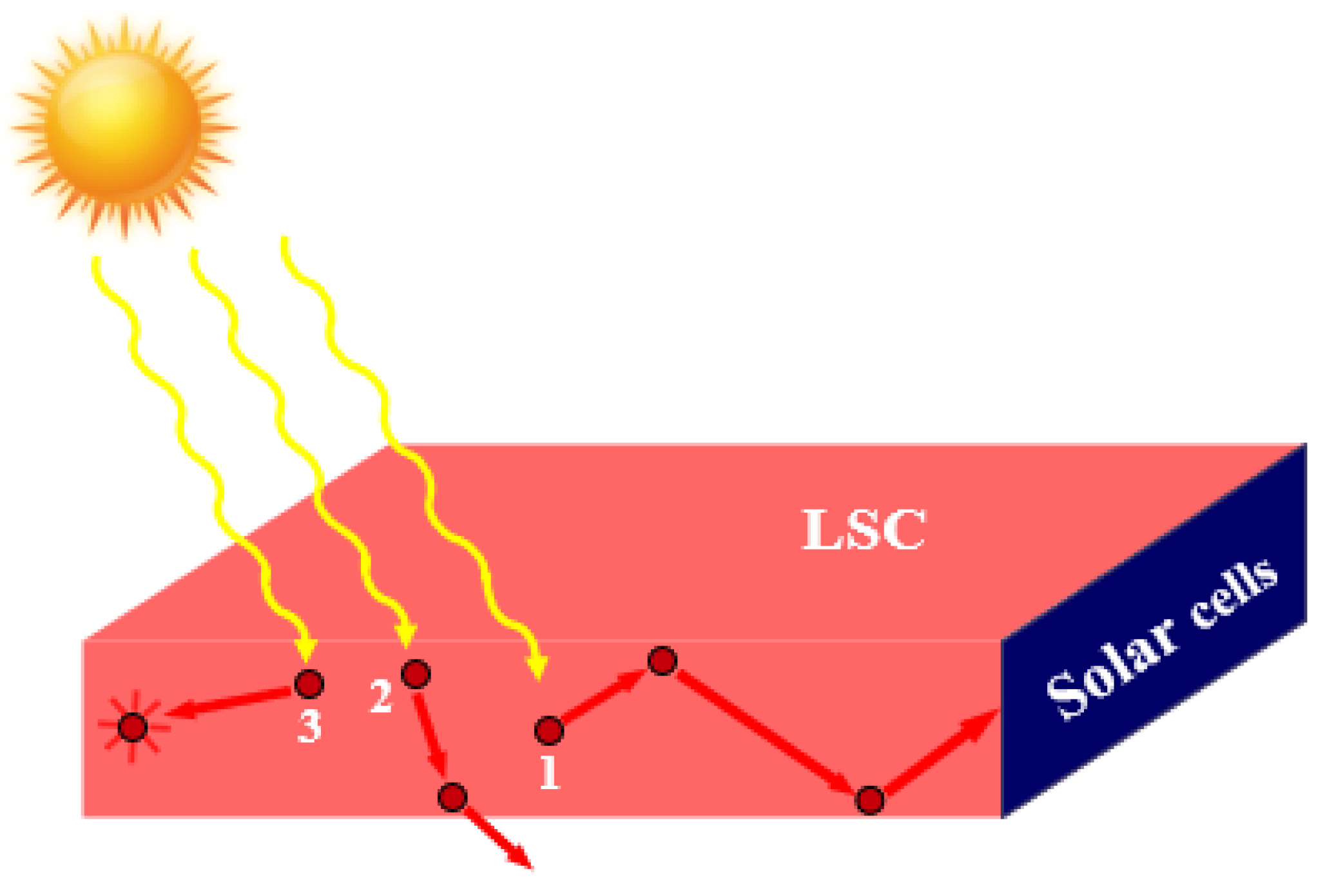
1. Introduction

The goal 7.2 of the 2030 Sustainable Development Agenda testifies that now, more than ever, it is necessary to satisfy the growing need for energy using renewable sources [1,2]. In particular, considering the amount of energy that strikes Earth’s surface every day, PhotoVoltaic (PV) technology could be one of the most relevant energy sources. This is confirmed by the considerable size reached in these years by PV technologies market, which nowadays amount to 7.6% of the energy produced by renewable non-combustible sources [3]. Among all PV technologies, Luminescent Solar Concentrators (LSCs) represent a promising way to widen the field of application of PV systems and increase the amount of energy produced by solar technologies [4]. The performance of standard PV technologies are highly affected by shading and, if bypass diodes or other bypass devices are not installed, the PV modules can suffer of permanent damage when shaded [5]. This is particularly true for high power modules, employed in solar power plants, or for high performance solar cells employed in aerospace applications [6,7,8]. LSC panels are instead extremely tolerant to shading, as they can exploit both direct and diffuse radiation [9]. Therefore, they are perfect candidates for Building Integrated PhotoVoltaic (BIPV) applications, especially in the countries with a high population density or in which diffuse solar radiation is dominant [10,11]. LSC panels are based on the coupling of a semi-transparent glass or plastic slab with PV cells. The slab is functionalized with fluorophores able to absorb a portion of the impinging light and then re-emit it as fluorescence light. Each time that the light is emitted by the fluorophores three different phenomena can occur: total internal reflection, escape-cone losses, and self-absorption (see Figure 1). Indeed, the fluorescent light is isotropically emitted and just a portion of it undergoes total internal reflection, the remaining one is lost through the so-called escape-cone. Both the escape-cone losses and the amount of light entrapped in the LSC depend on the slab material and then can be expressed as a function of the slab refractive index [12]. The self-absorption phenomenon is due to the partial overlap between the luminophores absorption and emission spectra, in fact if the Stokes shift is too small the luminophores inside the slab can absorb also fluorescence light, thus increasing the number of absorption events and the probability of escape-cone losses. The light that thanks to total internal reflection is trapped inside the slab is waveguided to its edges where usually PV cells are mounted. This configuration allows the conversion of light into electricity and minimize the area of the solar cell needed, thus leading to a potential reduction of the panel overall cost. The slab can be manufactured with various shapes and be functionalized by using different luminophore types like organic or inorganic dyes as well as quantum dots. Their optical properties affect the absorption and emission spectra of the LSC, changing its characteristic color [12]. LSC panels show a high PV conversion efficiency, as fluorophores realize a down-shifting of wavelengths that cross the slab, which guarantees an efficient filter against the solar UV radiation, and ensures to expose silicon (Si) solar cells to a wavelength range in which their External Quantum Efficiency (EQE) is higher [13,14].

The intrinsic optical transparency of LSC panels opens the possibility to install them where traditional PV technologies would not be suitable, exploiting the solar radiation not only for electrical energy production, but also to optimize the building thermal budget. Moreover, if installed on the roof of greenhouses, they can both contribute to supply the power needed by the greenhouse and increase the amount of light available for photosynthesis [15].

Considering the aforementioned properties, LCS panels are ideal to be installed in semi-transparent façades of new type of buildings, which could take advantage of BIPV technologies and could autonomously produce all or part of the energy they need. This could allow an increase of electricity generated from renewable sources, shifting the role of buildings form consumer to pro-sumer (producer and consumer) of energy [16,17].

In literature, there are many examples in which LSC panel characteristics are modified to increase the Optical Efficiency (OE) or the concentration factor of the system. Several are the studies in which each component of the LSC module is optimized to improve the system efficiency: the luminophores employed [18,19,20], the dimensions and shape of the luminescent slabs [21,22,23,24], and the types of solar cells used in the PV arrays [25,26,27]. Despite there is a clear understanding of the optimal solution combining all these features to lead to the highest efficiency, the industrial scalability and the availability of low-cost components is a key factor to unlock the potential of this technology. Presently, the price-to-watt ratio of commercial BIPV technologies range from 1.2 €/Wp, for glass-glass PV panels designed for architectural integration, to 8 €/Wp for PV glass based on a-Si technology [28].

Rafiee et al. work [29] shows that the LSC panels that are more scalable, and so suitable for BIPV applications, are based on organic dyes and Si solar cells. Based on this evidence the LSC panels presented in this research activity were functionalized with organic commercial dyes and coupled with commercial Si solar cells, as the purpose of this work was to develop devices that can be integrated in building semi-transparent façades. Therefore, all the configurations considered were designed to be as similar as possible to semi-transparent panels. As a further step towards industrial scalability, we studied different configurations where cell arrays were substituted with optical reflectors to minimize the overall system cost. Indeed, the reduction of the PV arrays number has a significant impact on the whole module cost. As a matter of fact, for the configurations presented in this work we estimated a price-to-watt ratio ranging from 13 €/Wp, for the configuration with the arrays along the four sides, to 7 €/Wp for the configuration with just one PV array. This estimation was done assuming a 30% margin on the direct costs, as there is no evidence of commercially available PV panels based on LSC technology. We present here the results we obtained for LSCs with cell arrays on four sides, on two sides and on just one side.

The LSC panel properties were first simulated to identify the configuration with the best efficiency/scalability trade-off, as the latter is an important feature that should be considered in view of a technology transfer from research to industrial scale. The panels performance was evaluated by analyzing different shading conditions, as they were tested not only under an ideal sunlight exposure (full lighting conditions), but also in real working conditions (partial shading). In fact, while the shading of standard PV flat modules has been widely investigated, literature lacks an in-depth analysis concerning this topic for LSC devices. Finally, some prototypes were assembled considering the simulation results and selecting the most promising designs.

2. Materials and Methods

2.1. Numerical Simulations

To evaluate how the concentrator geometry affects the power production, numerical simulations of light transport inside the LSCs were performed. The results presented in Appendix A guided us to simulate square-shaped LSC panels with an area of 25 × 25 cm² as smaller dimensions would still have spectral components of light affected by auto absorption, thus making obtained results difficult to project to larger size devices. In LSC panels with dimension of 25 × 25 cm² or wider, the spectral components affected by auto absorption reaching the solar cells become negligible with respect to the longer wavelengths showing no auto absorption, and thus these components of the fluorescence light can be assumed to undergo free propagation within the LSC slab. Therefore, in the optical simulation, a ray of light was considered lost only when it was absorbed by an absorbing surface or when it escapes through the escape-cone.

The relative values of the irradiance on the LSC side were obtained with a Montecarlo raytracing technique, and the relative short circuit current produced by each cell was given by the integral of the irradiance distribution over the cell length. Rays of light were generated inside the LSC with a uniform spatial and angular distribution; therefore, the path of each ray of light was a straight line that ended on a surface of the LSC. The variance in panel performance due to the light incidence angle was neglected as incidence angle modifier was already studied by Kanellis et al. [30]. Three different configurations of LSC panels were simulated, with four, two, and one PV arrays, respectively. The PV arrays were simulated along the LSC edges and in the configurations with one or two PV arrays, the missing ones were replaced by reflective surfaces. The basic PV array was 25 cm long and was composed by 10 photovoltaic cells connected in series, however, in this study were evaluated also configurations in which the number of cells per PV array has been reduced. The flow chart shown in Figure 2 summarizes the complete simulation procedure.

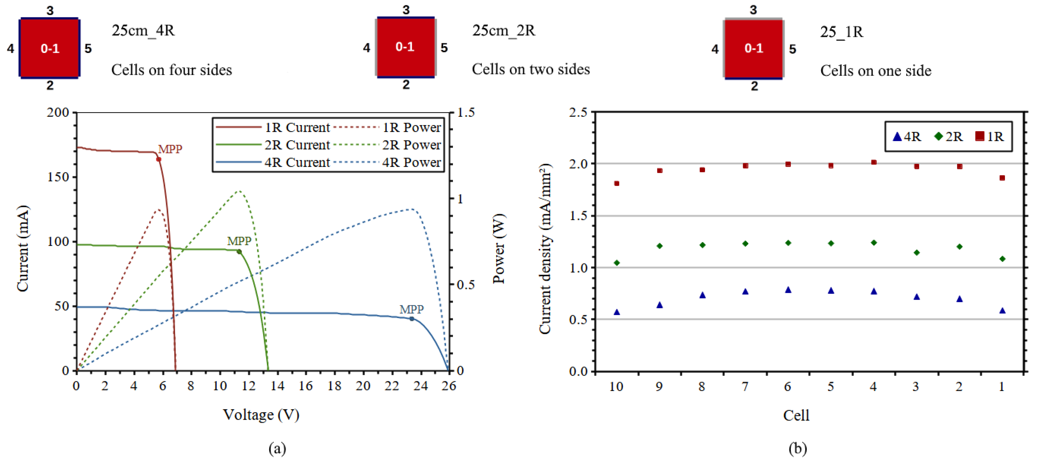
2.1.1. Simulated Electrical Performance

To evaluate LSC panel electrical performance, three types of surfaces were considered: refractive, reflective, and absorbing. Refractive surfaces represent the LSC-to-air interfaces where, depending on the LSC refractive index, the rays of light can undergo total internal reflection or exit from the slab surfaces. The reflective surfaces were used to simulate the LSC sides covered by the mirror films. When a ray of light struck a reflective surface, a random number between 0 and 1 was generated and, if it was higher than the surface reflectivity, the ray of light was considered as absorbed by the surface. Differently, the absorbing surfaces were representative of the solar cells, which were simulated as perfect absorbers.

The selected parameters for the simulations were the LSC refractive index, the mirror reflectivity, and the ray flux. The first was set at 1.488 at 650 nm [31], and the second was set at 0.95 according to the reflection properties of the dielectric mirror film used for the prototypes [32]. The ray flux was set to 1.6 × 10⁸ rays of light/m², thus ensuring a trade-off between the computational time and smoothing of the cell irradiance profile.

When a ray of light was absorbed or lost through the escape-cone, the software saved the path data, which consisted of the source point, the direction cosines, the points where the ray of light was reflected, the outgoing direction after each reflection, and the surface nature (reflective or absorbing). By analyzing these data, it is possible to generate the irradiance profile on each surface as well as to evaluate the number of rays of lights lost because of the escape-cone losses or the absorption by the reflective surfaces.

2.1.2. Simulated Impact of Shading

To evaluate LSC losses in efficiency because of the partial shading, irradiance profile on the PV cells array was simulated with the same parameters and methodology described in the Section 2.1.2, but under relevant shading conditions.

The reference design consists in the square LSC with PV arrays along the four sides, and without any reflective surface. This design has been taken as a reference because it represents the most common and spread LSC panel configuration used in transparent façades. As described in Section 2.1, the other simulated setups consist of LSC panels with cell arrays on one or two sides.

Depending on the arrangement of the cells in the LSC panels, it is possible to identify different shading situations. In the reference system equipped with four PV cell arrays, being symmetrical on two axes, any shading mode is equivalent. In the system with two PV arrays on opposing sides, two shading options are possible: across the arrays, and parallel to the arrays, because, due to system symmetry, it is not important which array is being shaded. In the system with only one PV array, three options are possible: the first one involves the shading across the array, whereas in the second one the shading is parallel to the PV array on the half of the slab opposite to the PV cells. The third shading mode involves the shading of the half surface that includes the PV array (Figure 3).

Obviously, the most critical situation is the shading across the PV array because the difference in the irradiance profile would lead to a strong current mismatch and, consequently, to a loss in the system efficiency.

2.2. Prototype Assembly Process

The modules consist of square slabs of PMMA (PolyMethylMethAcrylate) doped with a concentration of 300 ppm organic dye developed by BASF Corporation, and thus belonging to the commercial Lumogen^® F family: Violet 570, Green 850, Yellow 083, Orange 240, and Red 305. The latter four dyes are perylene-based, while Violet 570 is a naphtalimide-based one. The slabs (5 mm thick) were laser-cut with a size of 25 × 25 cm².

The LSC slabs were coupled with monocrystalline Passivated Emitter Rear Contact (PERC) silicon solar cells (SunPower C50) with dimensions of 23 × 8 mm², which were obtained by the mechanical cutting of 156 × 156 mm² area wafers [13]. The cells were arranged in arrays of 10 cells, connected in series, and soldered onto a Printed Circuit Board (PCB) 244 mm long.

The assembly of the cells soldered on the PCB represents the modular PV array. Further information about the electrical characterization of both the bare solar cells and the PV arrays can be found in the Supplementary Material (Figure S1). The modules were assembled mounting the PV arrays along the edges of the slabs, by using an optical UV glue (Delo Photobond GB368) and placing a high efficiency dielectric mirror film (DF2000MA, manufactured by 3M) along the sides without cells. The film consists in a dielectric mirror deposited on plastic layer with an overall thickness of 104 μm and a contact adhesive applied on it. The main feature of the mirror film is the high specular reflectivity. It shows a reflectivity higher than 90% in the 400–775 nm range, at an angle of incidence between 0 and 80° that helps to minimize the absorption losses even in case of multiple reflections [32]. The glue is a one-component UV-curing adhesive, specifically formulated to bond optical devices made of glass, plastic, or metal. This glue has a refractive index of 1.506 in the visible range, slightly higher than PMMA, but close enough to achieve a good optical coupling between the slab and the cells [33]. Figure 4 displays the pictures of the assembled prototypes in the different configurations.

2.2.1. Prototype Electrical Performance

The prototypes were placed on a dual-axis sun tracking system equipped with a pyranometer DeltaOhm LP Pyra 03 AV. The pyranometer was used to measure the incident global irradiance on the plane of the module. The I-V and P-V characteristic curves were measured by mean of a Keithley 2400 SourceMeter controlled by a custom Virtual Instrument written in LabView. The software automatically calculates all the parameters of the curve, such as the short circuit current, the open circuit voltage, the maximum power point, the voltage and current at maximum power point, and the Fill Factor (FF). The software saves automatically the I-V curve data and performs batch and periodic 4-wires measurements. The efficiency of the prototypes was obtained analyzing both the I-V curves and the irradiance data, which was measured by the pyranometer.

The assessment of the electrical performance of the panels was carried out by measuring the I-V curves of the LSC panels under natural sunlight. Thus, to guarantee that the LSC performance were not affected by the sunlight incidence angle the panels were placed on a sun tracking system, which also allows to maximize the irradiance received by the prototypes.

As reported in the SunPower C50 datasheet [13] the EQE of the PV cells mounted on the prototypes is almost constant from 400 nm to 1000 nm, thus the current produced by the cells can be considered directly proportional to the intensity of light that strikes the cells. Therefore, the OE of the LSC panel can be expressed as defined by Inman et al. [21], namely as the short circuit current produced by the LSC panel, I_SCLSC, divided by the product between the same quantity produced by the bare PV array, I_SCPV, and the geometric factor G:

OE = I_SCLSC [A]/(I_SCPV [A] · G),

(1)

G is the ratio of the illuminated LSC top surface area to that of the edges covered by PV cells, so its value is a function of both prototype configuration and shading condition. In this way, the OE includes the dependence of PV cells Quantum Yield (QY) from the different wavelengths.

Another quantity used to define the performance of an LSC panel is the Power Conversion Efficiency (PCE), which can be expressed by Equation (2), and compares the electrical power, which is supplied by the LSC panel, to the radiative power striking on it:

PCE = (I_MPP [A] · V_MPP [V])/(GNI [W/m²] · cos(θ) · A [m²]),

(2)

where I_MPP, and V_MPP are respectively the maximum power point current and voltage, GNI is the Global Normal Irradiance; namely the total irradiance that reaches a surface perpendicular to the line joining the Earth and the Sun. A is the area of the LSC top surface, and θ is the angle between the surfaces used to compute the GNI and the LSC top surface. The prototype electrical performance was tested under a GNI equal to 630 W/m².

2.2.2. Impact of Shading on the Prototypes

In order to study a maximized effect of shading, the tests were performed by covering half of the concentrator with black absorber. This precaution is needed to avoid that the light emitted by self-absorption and lost from the escape-cone could be reflected by the shading surface. The covering of the half of the system is obviously a situation of extreme shading, which should be avoided by a proper installation of the modules. Nevertheless, modules working fairly in this situation could be used on purpose when partial shading is unavoidable, and when the installation of other systems is economically infeasible. The symmetry conditions, which led to different shading configuration, are the same presented in Section 2.1.2.

3. Results and Discussion

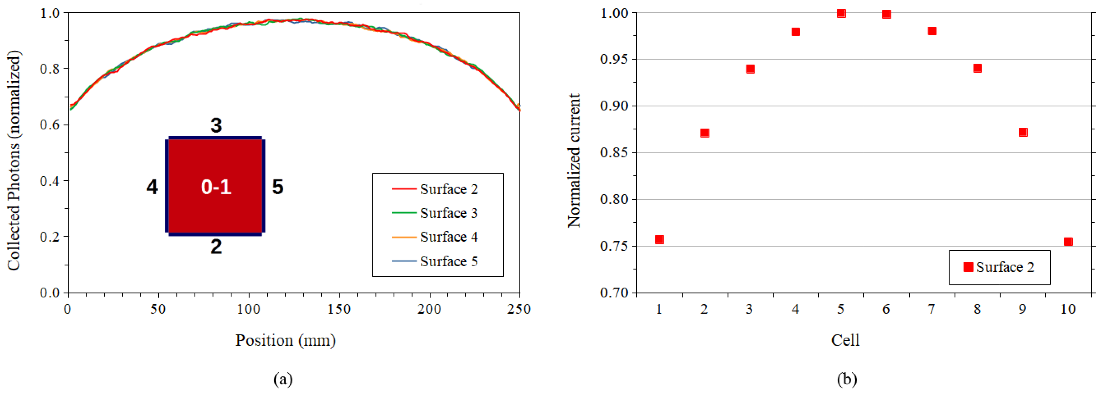
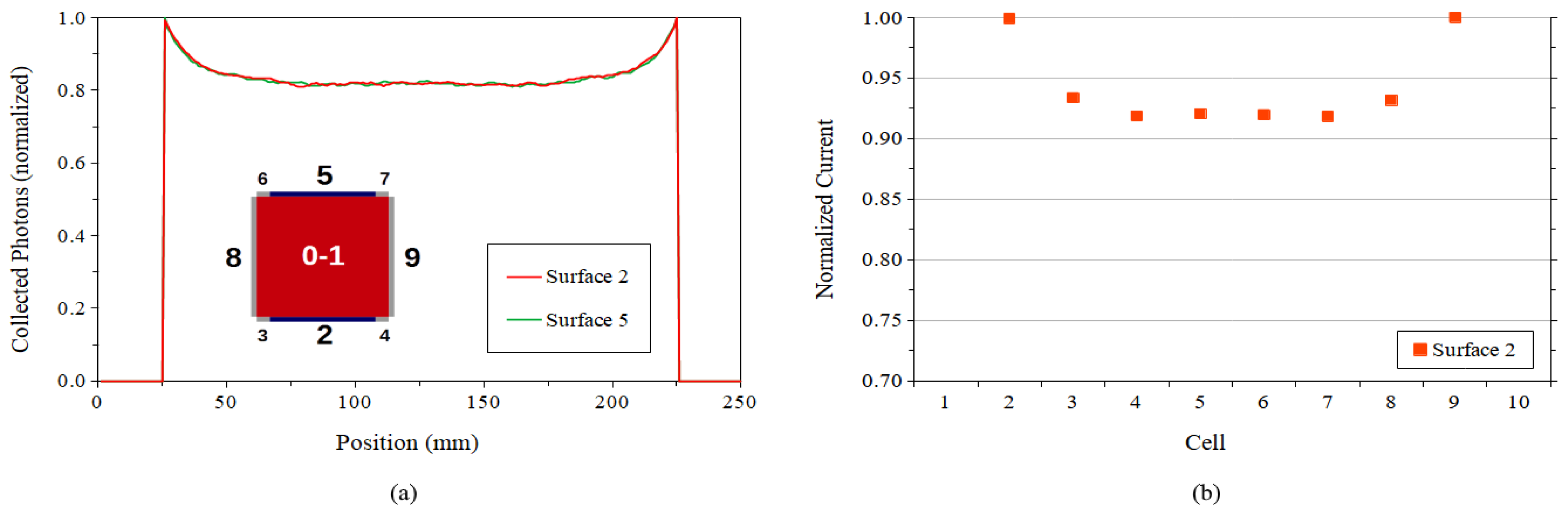
3.1. Simulated Electrical Performance

The first simulated LSC had four arrays, one for each side, with 10 cells per array. As mentioned above, such a configuration represents a reference to evaluate the effectiveness of the others. The arrays on each side allow the maximum absorption but as shown in Figure 5a, the irradiance profile is uneven, and seems to follow a cosine-like function. This irregularity led to a mismatch in current production, approximately equal to 33%, between the central cells and the ones at the ends of the same array (Figure 5b).

Therefore, if the cells are connected in series, this configuration turns to be unprofitable unless bigger cells are employed at the array ends. Differently, cells of equal size could be used if connected in parallel, since their operating voltage is barely affected by such mismatch [34].

Unfortunately, the use of cells of various sizes would make impractical the scaling up of the concentrator to larger areas. In fact, to correctly fit the different irradiance levels across the same side, the larger cells should be 50% longer than the smallest ones, making them extremely fragile. Moreover, the maximum size that can be handled by the assembling machines is limited. Thus, if the largest cell size is limited, an approach with cells of different sizes requires the use of more cells to cover the same length. Using a large number of cells, also the option to connect all the cells in parallel would be equally not convenient. It would result in an output with a high current and low voltage, which requires the use of conductors with large cross section and leads to significant losses in dc-dc or dc-ac conversion [34]. Removing one cell per array and replacing them with reflective films have a dramatic effect on the irradiance profile, as depicted in Figure 6.

The irradiance profile shows high variations—greater than 35%—among the different surfaces, which is even worse than the reference. Therefore, this strange design has hardly a practical interest.

In Figure 7, are displayed the results concerning an LSC panel with four arrays, each one with 8 cells. Covering the corners of the LSC with reflective mirrors can be considered an advantageous alternative for several reasons: the number of cells used for each module is decreased, the corners represent the areas with lowest irradiance, and configuration symmetry is restored. The coverage of the LSC corners presents a couple of problems. The former is the small current mismatch among the cells, around 6%. The latter, and most concerning one, is represented by the cells to mirror junction, which make this configuration extremely sensitive to assembly errors. In fact, any error would result in a significant current loss, as testified by the sharp peaks at the cell-mirror interface. Therefore, also this configuration is of limited practical interest.

After these, a configuration in which two PV arrays were replaced by reflective films was tested. The addition of the reflecting film on two sides has a great impact on the irradiance profile (see Figure 8a). In fact, the difference in irradiance between the center and the ends becomes less than 3%, with respect to the 50% shown by the reference configuration. This close-to-ideal irradiance profile comes at the cost of absorption that is caused by the reflective surfaces, whose reflectivity have been estimated around 95%. This means that photons undergoing multiple reflections on the sides are likely to be lost due to absorption by the reflective films. Figure 8b shows that the current mismatch among the cells is minimal: this small variation in current production is probably less noticeable than the statistical variation between the cells and the effect of small assembly defects. The uniformity of the current profile results in a higher efficiency of the module.

Looking at the good performance of the configuration with two reflective sides, a configuration with two arrays with eight cells each was simulated. The intention was, as before, to reduce the number of cells employed in the LSC panel. The reflective sides help to even out the irradiance profile, but this process results again in a higher current mismatch between the cells (Figure 9). The widening of the peak at the cells-to-mirror junction causes an increase in the current produced by the extreme cells which results in an increased mismatch between the cells.

Finally, a configuration with three sides covered by a reflective film and one by an array with 10 cells was simulated. There is no noticeable improvement of the irradiance profile with respect to the configuration with two PV arrays (Figure 10), but it can be observed a higher absorption that makes this design less efficient than the one displayed in Figure 8. This configuration anyway requires only a fourth of the cells employed in the reference and hence represents the most affordable if the price-to-watt ratio is considered.

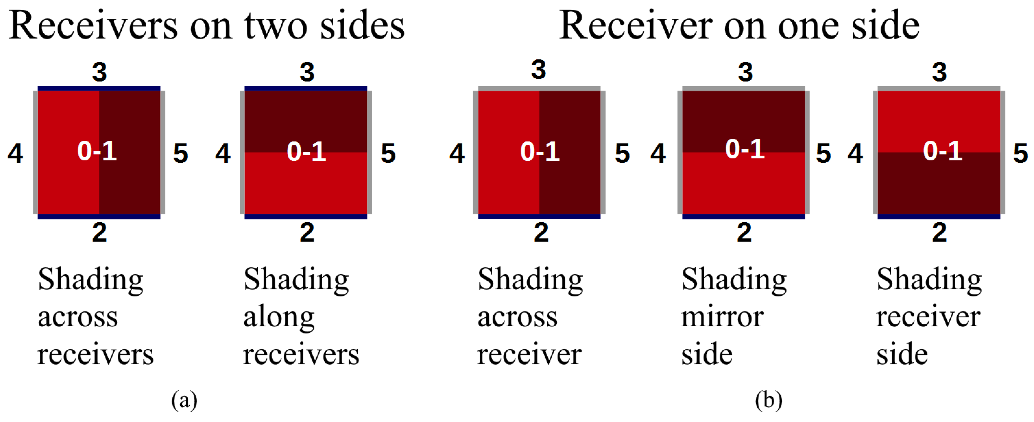
3.2. Simulated Impact of Shading

The LSC panels shading performance was simulated just referring to the configuration with four, two and one PV arrays, having 10 cells each. Indeed, considering the results presented in Section 3.1, these seems to be the most interesting and promising configurations.

In Figure 11 are displayed the results for the configuration with four PV arrays, which was taken as a reference. In addition to the irradiance profiles on the PV arrays, the rays of light lost from the escape-cone, and the rays of light absorbed by the reflective surfaces are shown.

Because of the symmetry, the half-shaded arrays collect the same irradiance profile, which presents very large variations. As predicted, this led to a strong current mismatch and consequently to a loss in the system efficiency. The unshaded side presented an irradiance profile identical to the completely unshaded condition. Surprisingly, the lowest irradiance values are located on the half-shaded arrays, while the completely shaded one shows a relatively uniform irradiance profile. Therefore, the limiting factor for the system power output is not the completely shaded array.

As expected, looking at the irradiance profiles, the current produced by each cell shows the highest value for the cells 5 and 6 of surface 4, which represents the unshaded array. The lowest values are the ones registered for cell 10 of surfaces 2 and 3, which represent the half-shaded arrays. With this configuration, the best cells produced four times the current of the worst ones, leading to a dramatic power loss.

When two arrays are replaced by the mirrors, and the shading is parallel to them, the mismatch seen in the last case is effectively mitigated (Figure 12). The irradiance peak is located at the illuminated end of the arrays and the difference between the maximum and minimum values is 2.4 times. With a reflectance of 0.95, the absorption caused by the reflective surfaces is negligible, and its effect becomes acceptable if the increased flatness of the irradiance profile is considered. Looking at the expected current production, the mismatch reduction is evident: in this case, the difference is reduced to 2.4 times, leading to a significant improvement in system efficiency.

Shading simulation along the arrays does not seem to significantly affect the performance of this system. Indeed, a difference in irradiance between the two sides is anyway present but is not as dramatic as in the previous configuration of shading across the arrays. The irradiance profiles on the two surfaces hosting the cells show the same difference of 3% between the highest and lowest values previously seen without the shading. In this case, the mismatch between the arrays is limited to 10%, as displayed in Figure 13. This result testifies an efficiency loss reduction and allows the system to maintain good performance even under partial shadowing.

The results for the configuration with one array are shown in Figure 14. For the simulation in which the shading is applied across the array, the addition of a third reflective surface results in a further flattening of the irradiance profile. In this case, the difference between the highest and lowest irradiance values is limited to 50%: a remarkable result for such an extreme shading pattern. As expected, looking at the irradiance profile, the current mismatch among the cells is the lowest seen so far for this shading pattern, with the best performing cells producing 1.5 times the current of the cell with the lowest current.

As displayed in Figure 15, the configuration with one receiver presented a remarkable tolerance to shading, especially when it is along the array on the mirror side. The regularity of the irradiance profile reflects on a negligible mismatch in the current produced by the different cells. Therefore, with this shading pattern, the system shows no efficiency loss.

As in the previous case, the shading of the array on the cells side leads to a flat irradiance profile, and to a match in the current produced by the cells. Looking at all the shading patterns, this system performs better than the other configurations under partial shading (see Figure 16) and, adding the reduced cost and ease of assembly and wiring, it is clearly the best candidate for industrialization.

Among the various setups evaluated in the numerical simulations, the best theoretical performance was achieved by the configuration with two arrays, which balances the good uniformity in the irradiance profile with reduced losses caused by multiple reflections on the reflective layers. The setup with the cells placed only on one side of the slab have an irradiance profile similar to the system with two arrays, but with a lower power output. The power output decrease is caused by the increased number of reflections along the sides, and therefore by the increased chances of absorption. However, the system with one array shows the lowest current mismatch among the cells. As the simulations suggested, the mirrors improve greatly the uniformity of the irradiance profile, and the system with cells on two sides is the configuration yielding the highest efficiency.

3.3. Prototypes Electrical Performance

LSC panel prototypes were assembled with the same dimension and shape of the simulated devices. However, before testing the prototype electrical performance the PCE of LSCs functionalized with different dyes was evaluated. Figure 17 shows different efficiency values obtained using Equation (2).

Since the most efficient LSC panels was the one functionalized with the Lumogen^® F Red 305 dye, all the prototypes were realized by using this specific dye. In fact, its emission peak, reported in the Lumogen^® F Red 305 datasheet [35], allows a better harvesting of the light emitted by the sun. Further information on the optical characterization of the functionalized PMMA slab can be found in the Supplementary Material (Figure S2).

As in the simulations, the configuration with the arrays on the four sides is taken as a reference. In the relative I-V curve, shown in Figure 18, a hump is clearly visible: it is due to the mismatch in the current produced by the extreme cells and the ones at the center of each side. An estimation of the irradiance that impinges on the cells at the far ends of the arrays can be obtained taking the short circuit current as a reference and considering that the exposed surface of the cells is only 5 mm out of 8 mm. The estimate for the irradiance at the corners is I ≈ 1.2·I₀, where I₀ represents the irradiance on the LSC surface. For the central cells, this value increases to 1.67·I₀ as expected from the irradiance profile of the corresponding simulation (Figure 5). The efficiency of this configuration is 1.83% with a FF equal to 0.70.

Figure 19 testifies that the configuration with two arrays, performed better than the reference one. The efficiency rises up to 1.93% and the FF increases to 0.79, even if half of the cells has been employed and the produced power is increased too. However, a small amount of current mismatch appears to be present anyway. This is caused by the reflectivity of the mirror film, which is lower than expected, and a bending of the arrays due to the soldering technique. The first one leads to a reduction of the irradiance on the cells close to the mirror. The second one does not ensure a reliable optical coupling of the solar cells at the far ends of the array, preventing an optimal optical coupling.

In this configuration, the short circuit current scales almost linearly with respect to the reference configuration and the increase in concentration is 1.97×, while the irradiance is 2.36∙I₀.

In the configuration with just one array, the efficiency is not as high as in case of the configuration with two arrays. Indeed, it decreases to 1.63%. Nevertheless, this configuration is extremely interesting because the decrease in efficiency is counterbalanced by the easier assembling process and by the lower number of cells employed. In fact, the placement of the cells along only one side greatly simplifies the wiring process, which is an important aspect in solar panels, and significantly decreases the module cost.

Figure 20 shows that the current mismatch between the cells is negligible and, as in the previous configuration, thanks to the high irradiance on the cells the FF is 0.79, which is a very high value for silicon solar cells.

The concentration factor is 3.5× with respect to the configuration with the cells along the four sides, and the irradiance is approximately 4.2∙I₀. This value is non-ideal for cells designed to work at one sun, in particular for the PERC cells used for these tests. These cells perform well at one sun, but at higher irradiance levels their performance decreases sharply because they are not designed to conduct high current densities. Back-contact solar cells show lower efficiency under concentration because of higher bulk resistance optimized for 1-sun operation. On these grounds, the use of solar cells that could be optimized for low concentration applications would increase the efficiency of this last configuration [36].

The results presented in

Table 1. Electrical performance of unshaded LSC panels under a GNI equal to 630 W/m^2.

Configuration	VOC (V)	ISC (mA)	VMAX (V)	IMAX (mA)	PMAX (mW)	FF	OE (%)	PCE (%)	€/Wp
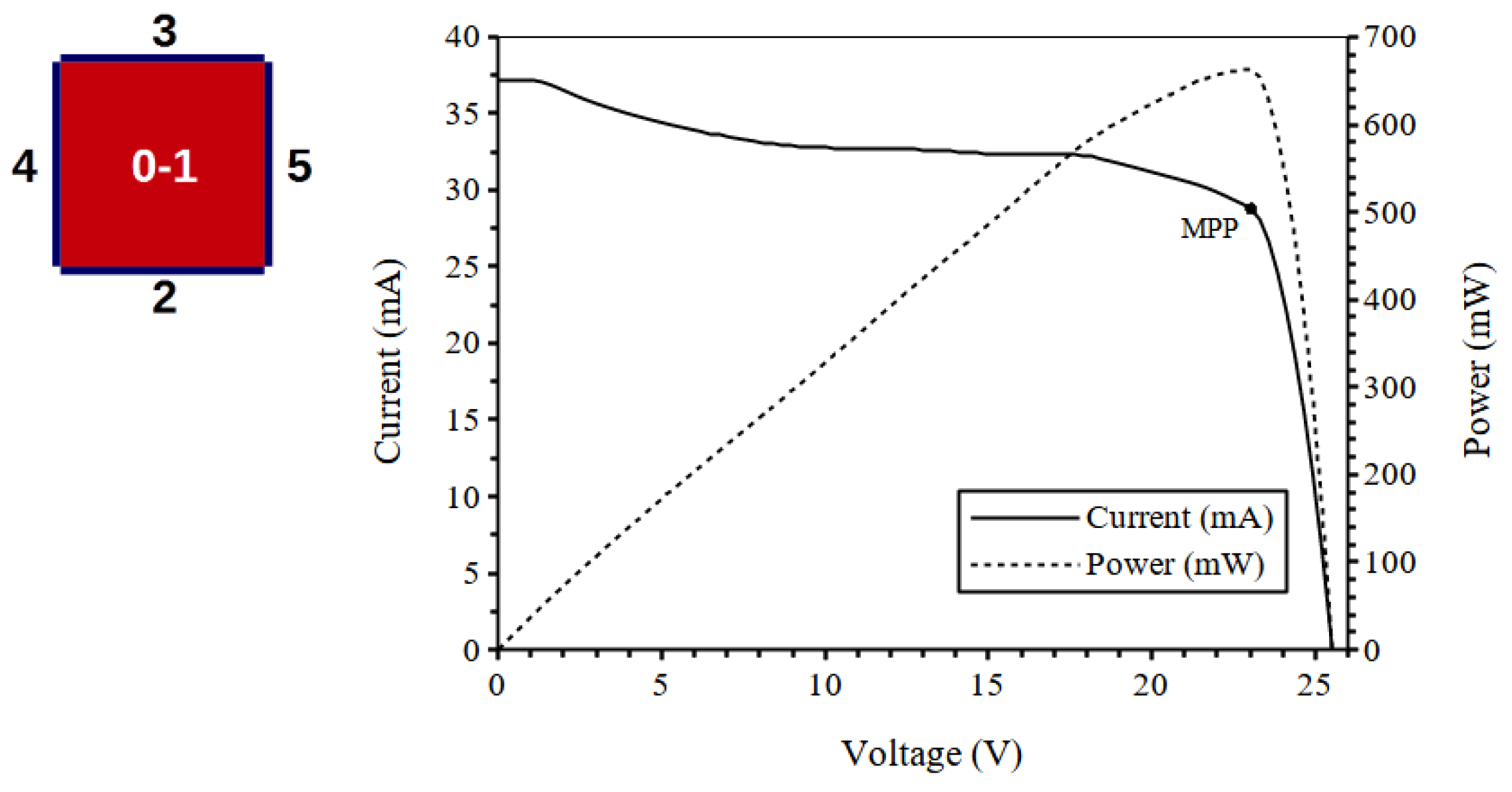
4 PV arrays	25.55	37.16	23.03	28.79	663	0.70	9.1	1.83	13
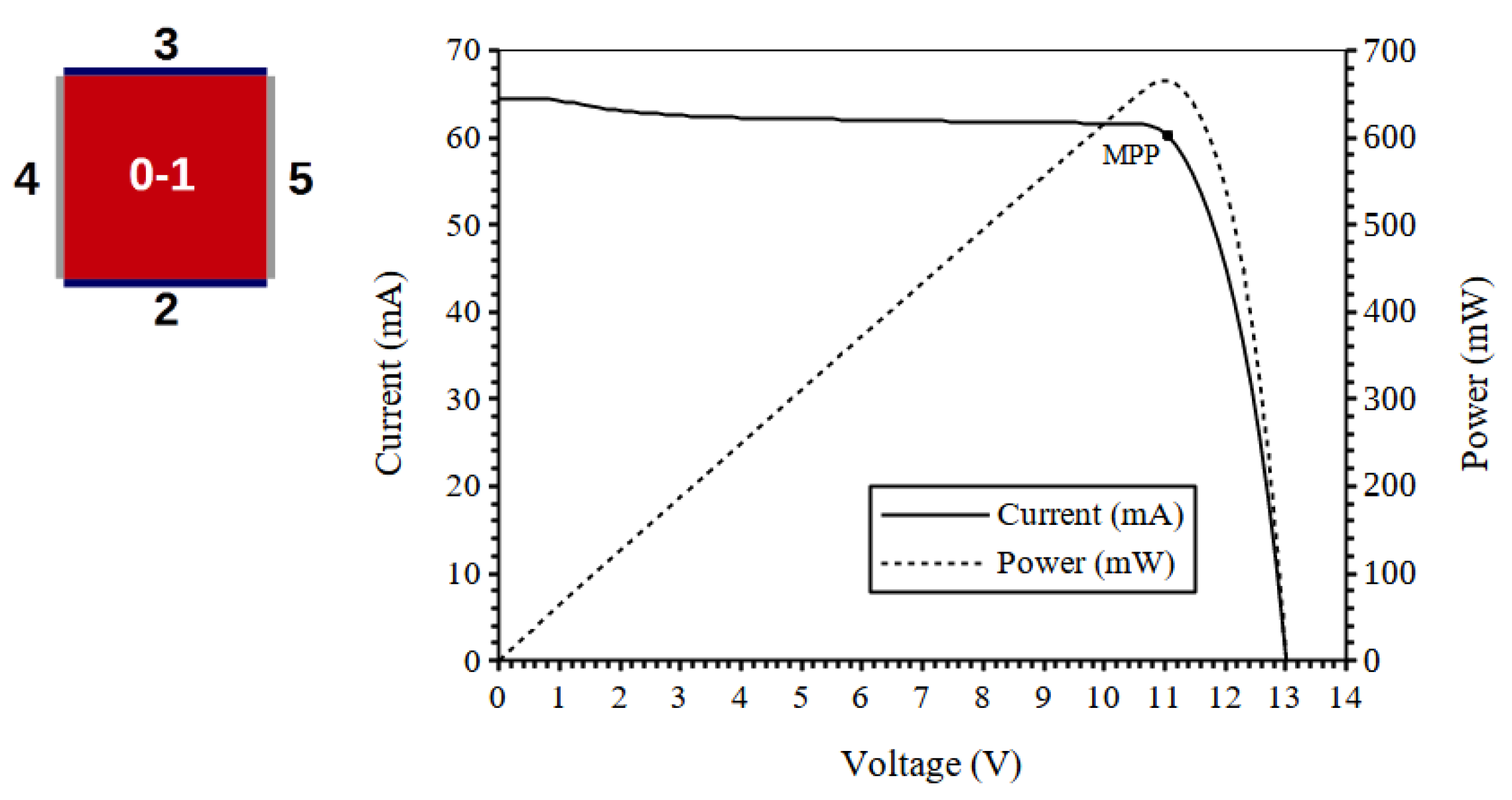
2 PV arrays	13.06	64.54	11.05	60.22	665	0.79	7.7	1.93	8
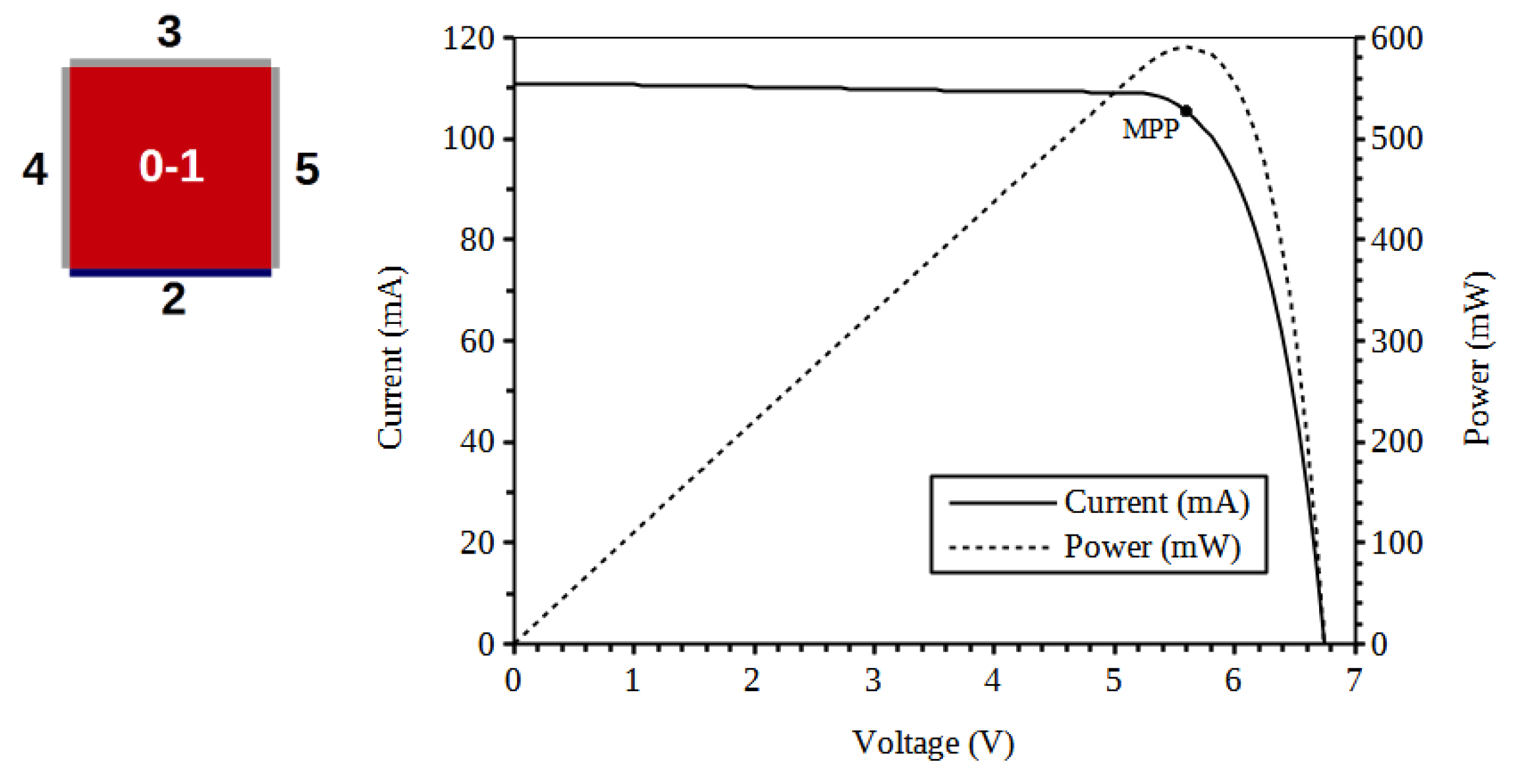
1 PV array	6.77	110.91	5.60	105.50	590	0.79	6.4	1.63	7

proved that the systems assembled using just one or two arrays can provide a power output comparable to the reference configuration, at a fraction of the cost and with improved ease of wiring. These evidences are corroborated also by the results displayed in Figure 21a, which are the characteristic curves of the three configurations under one sun illumination. Figure 21b confirms that in the configurations with one and two receivers the current mismatch between the cells is reduced, thus decreasing the module efficiency losses.

3.4. Impact of Shading on the Prototypes

As predicted by the simulation, the shading has a dramatic effect on the reference system. Indeed, as depicted in Figure 22, when two arrays are half-shaded and another one is fully shaded, the consequent current mismatch hinders the performance. Thus, the FF decreases to 0.52, and the efficiency is halved with respect to full exposure.

Differently, the configuration with two arrays is more tolerant than predicted by the simulations. If the shading is applied across the arrays, the highest current is produced by the cells at the center of the illuminated area, while the minimum is produced by lateral ones (see Figure 23). The cells at the shaded far end of the arrays (n.10 for surface 2 and n.1 for surface 3) are the limiting factor for the system power production, because both the cells and the arrays are connected in series. The cell numbering in the arrays is not symmetrical, so the cells of the array placed on surface 3 are numbered backwards. It appears evident that this configuration performs much better than the reference one, despite the non-uniform illumination of the cells. Indeed, with respect to the unshaded configuration, the FF is higher (0.75), and the efficiency is only 50% lower.

If the shading is applied along the arrays, the current and the irradiance profile are much more uniform, as displayed in Figure 24. The FF remains the same, whereas the efficiency rises to 1.59%. Even if one array is completely shaded, the cells producing less current, and therefore limiting the overall system power production, are anyway producing more current than in the previous case (25 mA vs. 19 mA, a significant 32% increase). As expected, the efficiency is just 20% lower than that one in the unshaded condition, but the remarkable result is that, by using half of the arrays, this configuration produces a power output 69% higher than the reference one.

Looking at the results obtained through the simulations, the configuration with just one array is expected to be the most efficient under all the shading conditions. Even in the most critical one, that is the shading across the array. Experimental evidence shown in Figure 25, testify that in this configuration the system performs remarkably well with a FF higher than 0.80, and an efficiency equal to 1.23%. The current profile, measured by using the prototype, is in good agreement with the irradiance profile obtained by the simulations (see Figure 10) and, as expected, there is a ratio of two between the current produced by the best and worst cells of the arrays.

In the other two configurations, instead, the current profile is uniform and, as is shown in Figure 25b, the current mismatch is around 10%. In fact, the current produced by the cells at the center is 10% higher with respect to the ones at the far edges. The mismatch is higher than expected, and it is most likely caused, once again, by the lower mirror reflectivity and by the non-optimal optical coupling of the cells, due to the bending of the array.

Figure 25a shows that when the half surface opposed to the array is shaded, the I-V curve of the system is almost impossible to tell apart from that measured in an unshaded condition. In this case, the efficiency is even higher (1.86%) because this shading configuration reduces the self-absorption contribution of the overall system. The same happens for the configuration in which the shading is applied along the array side. However, because in this case the photons have to travel a longer path before being absorbed (more reflections), the chance of self-absorption is higher, and both the power production and the efficiency are lower than in the previous case. The efficiency decreases to 1.46% as opposed to the FF that is equal to 0.78 for both configurations. The results that are displayed in Figure 25 are anyway very promising for a system whose cells are kept completely shaded.

Results summarized in

Table 2. Electrical performance of shaded LSC panels under a GNI equal to 630 W/m².

Configuration	VOC (V)	ISC (mA)	PMAX (mW)	VMAX (V)	IMAX (mA)	FF	OE (%)	PCE (%)
4 PV arrays shading across the receivers	24.02	13.54	168	16.56	10.14	0.52	8.5	0.93
2 PV arrays shading across the receivers	12.58	23.01	219	11.47	19.09	0.75	7.1	1.23
2 PV arrays shading along the receivers	12.55	31.02	285	11.18	25.44	0.75	7.3	1.59
1 PV array shading across the receiver	6.43	40.40	212	5.73	37.07	0.82	5.4	1.23
1 PV array shading along the receiver: mirror side	6.47	60.37	306	5.35	57.12	0.78	6.0	1.86
1 PV array shading along the receiver: receiver side	6.40	48.72	244	5.29	46.16	0.78	4.8	1.46

corroborates the hypothesis that the introduction of reflective layers improves the LSC panel performance also in the case of partial shading, as their presence increases the uniformity of the irradiance profile, thus reducing losses caused by current mismatch.

4. Conclusions

The results presented in this work highlight that Luminescent Solar Concentrators are a promising technology well suited for building integration. Most of the research about LSCs is currently focused on the development of dyes with low self-absorption or dye alignment, whose purpose is the reduction of the self-absorption losses, and the consequent increase in the system efficiency [37]. Presently, the main drawback of LSCs is their high price-per-watt ratio. In order to improve their appealing to the market, it is mandatory to reduce as much as possible the price difference between a normal transparent and a LSC façade.

The difference between the simulations and the real performance of the modules can be attributed to several factors. Among them, the most significant are a mirror reflectivity lower than the expected and minor assembly errors. These are caused by the bending of the arrays, which resulted in a non-optimal optical coupling between the LSC and the cells at the far ends of the arrays. The increase in concentration factor, which is shown by the systems employing mirrors, is close to the expected value: 1.97× and 3.5× for the configurations with two and one array, respectively. The irradiance along the cells side of the LSC with three reflective sides have been estimated to be 4.2 times greater than the solar irradiance on the LSC surface.

Tests performed in case of shadowing provided two remarkable results. The first one is that in this case the differences between the simulation and the measurements are highly reduced, thus leading to a good accordance between the simulations and the measurements performed on the prototypes. The second result concerns the systems assembled with the reflective films, which perform very well when shaded. In particular, the configuration with the cells on one side have shown the highest efficiency in all shading configurations. The demonstration that, despite the illumination conditions, the systems that employ a small number of cells can yield to a higher efficiency than a traditional system represents a significant result. In fact, any reduction in the number of cells implies not only a lower cost of the components, but also a faster, and hence cheaper, assembly process.

Having proved that the configurations with reflective films had a better price-to-efficiency ratio in the tested shading conditions than the system with cells placed along four sides, it would be interesting to apply this configuration to larger area LSC panels. Indeed, as mentioned in Section 2.1, square LSC panels of 25 cm side were chosen as their properties can well represent the optical properties of wider LSCs, even if their dimensions severely limit their use in the building sector.

References

- United Nations. Sustainable Development Goals. Available online: https://www.un.org/sustainabledevelopment/energy/ (accessed on 5 May 2020).
- Almeida, C.M.V.B.; Agostinho, F.; Huisingh, D.; Giannetti, B.F. Cleaner Production towards a Sustainable Transition. J. Clean. Prod. 2017, 142, 1–7. [Google Scholar] [CrossRef] [Green Version]
- International Energy Agency, Market Analysis and Forecast from 2018 to 2023. Available online: https://www.iea.org/data-and-statistics/?country=WORLD&fuel=Energysupply&indicator=Renewableelectricitygenerationbysource(non-combustible) (accessed on 5 May 2020).
- Goetzberger, A.; Greube, W. Solar Energy Conversion with Fluorescent Collectors. Appl. Phys. 1977, 14, 123–139. [Google Scholar] [CrossRef]
- Dhere, N.G.; Shiradkar, N.; Schneller, E.; Gade, V. The Reliability of Bypass Diodes in PV Modules. Reliab. Photovolt. Cells Modul. Compon. Syst. VI 2013, 8825, 88250I. [Google Scholar] [CrossRef]
- Tajmar, M.; Arriaga, G.S. A Bare-Photovoltaic Tether for Consumable-Less and Autonomous Space Propulsion and Power Generation. Acta Astronaut. 2020, 180, 350–360. [Google Scholar] [CrossRef]
- Papež, N.; Gajdoš, A.; Dallaev, R.; Sobola, D.; Sedlák, P.; Motúz, R.; Nebojsa, A.; Grmela, L. Performance Analysis of GaAs Based Solar Cells under Gamma Irradiation. Appl. Surf. Sci. 2020, 510, 145329. [Google Scholar] [CrossRef]
- Papež, N.; Gajdoš, A.; Sobola, D.; Dallaev, R.; Macků, R.; Škarvada, P.; Grmela, L. Effect of Gamma Radiation on Properties and Performance of GaAs Based Solar Cells. Appl. Surf. Sci. 2020, 527, 146766. [Google Scholar] [CrossRef]
- van Sark, W.G.J.H.M.; Barnham, K.W.J.; Slooff, L.H.; Chatten, A.J.; Büchtemann, A.; Meyer, A.; Mccormack, S.J.; Koole, R.; Farrell, D.J.; Bose, R.; et al. Luminescent Solar Concentrators—A Review of Recent Results. Opt. Express 2008, 16, 21773–21792. [Google Scholar] [CrossRef]
- Pagliaro, M.; Ciriminna, R.; Palmisano, G. BIPV: Merging the Photovoltaic with the Construction Industry. Prog. Photovolt. Res. Appl. 2010, 18, 61–72. [Google Scholar] [CrossRef]
- Debije, M.G.; Verbunt, P.P.C. Thirty Years of Luminescent Solar Concentrator Research: Solar Energy for the Built Environment. Adv. Energy Mater. 2012, 2, 12–35. [Google Scholar] [CrossRef]
- Rowan, B.C.; Wilson, L.R.; Richards, B.S. Advanced Material Concepts for Luminescent Solar Concentrators. IEEE J. Sel. Top. Quantum Electron. 2008, 14, 1312–1322. [Google Scholar] [CrossRef]
- SunPower Technical Data Sheet: C50 Solar Cell Mono Crystalline Silicon 2010. Available online: http://grubald.free.fr/Photovoltaique/pdf/c50solarcell.pdf (accessed on 2 February 2021).
- Tonezzer, M.; Gutierrez, D.; Vincenzi, D. Luminescent Solar Concentrators—State of the Art and Future Perspectives. In Solar Cell Nanotechnology; Scrivener Publishing LLC: Beverly, MA, USA, 2013; pp. 293–315. ISBN 9781118845721. [Google Scholar]
- Weber, W.H.; Lambe, J. Luminescent Greenhouse Collector for Solar Radiation. Appl. Opt. 1976, 15, 3–4. [Google Scholar] [CrossRef]
- Liserre, M.; Sauter, T.; Hung, J.Y. Future Energy Systems: Integrating Renewable Energy Sources into the Smart Power Grid Through Industrial Electronics. IEEE Ind. Electron. Mag. 2010, 4, 18–37. [Google Scholar] [CrossRef]
- Zarcone, R.; Brocato, M.; Bernardoni, P.; Vincenzi, D. Building Integrated Photovoltaic System for a Solar Infrastructure: Liv-Lib’ Project. Energy Procedia 2016, 91, 887–896. [Google Scholar] [CrossRef] [Green Version]
- Slooff, L.H.; Bende, E.E.; Burgers, A.R.; Budel, T.; Pravettoni, M.; Kenny, R.P.; Dunlop, E.D.; Büchtemann, A. A Luminescent Solar Concentrator with 7.1% Power Conversion Efficiency. Phys. Status Solidi (RRL) Rapid Res. Lett. 2008, 2, 257–259. [Google Scholar] [CrossRef] [Green Version]
- Goldschmidt, J.C.; Peters, M.; Bösch, A.; Helmers, H.; Dimroth, F.; Glunz, S.W.; Willeke, G. Increasing the Efficiency of Fluorescent Concentrator Systems. Sol. Energy Mater. Sol. Cells 2009, 93, 176–182. [Google Scholar] [CrossRef]
- Bomm, J.; Büchtemann, A.; Chatten, A.J.; Bose, R.; Farrell, D.J.; Chan, N.L.A.; Xiao, Y.; Slooff, L.H.; Meyer, T.; Meyer, A.; et al. Fabrication and Full Characterization of State-of-the-Art Quantum Dot Luminescent Solar Concentrators. Sol. Energy Mater. Sol. Cells 2011, 95, 2087–2094. [Google Scholar] [CrossRef] [Green Version]
- Inman, R.H.; Shcherbatyuk, G.V.; Medvedko, D.; Gopinathan, A.; Ghosh, S. Cylindrical Luminescent Solar Concentrators with Near-Infrared Quantum Dots. Opt. Express 2011, 19, 24308. [Google Scholar] [CrossRef]
- Zhang, J.; Wang, M.; Zhang, Y.; He, H.; Xie, W.; Yang, M.; Ding, J.; Bao, J.; Sun, S.; Gao, C. Optimization of Large-Size Glass Laminated Luminescent Solar Concentrators. Sol. Energy 2015, 117, 260–267. [Google Scholar] [CrossRef]
- Bronstein, N.D.; Yao, Y.; Xu, L.; O’Brien, E.; Powers, A.S.; Ferry, V.E.; Alivisatos, A.P.; Nuzzo, R.G. Quantum Dot Luminescent Concentrator Cavity Exhibiting 30-Fold Concentration. ACS Photonics 2015, 2, 1576–1583. [Google Scholar] [CrossRef]
- Vishwanathan, B.; Reinders, A.H.M.E.; de Boer, D.K.G.; Desmet, L.; Ras, A.J.M.; Zahn, F.H.; Debije, M.G. A Comparison of Performance of Flat and Bent Photovoltaic Luminescent Solar Concentrators. Sol. Energy 2015, 112, 120–127. [Google Scholar] [CrossRef] [Green Version]
- Currie, M.J.; Mapel, J.K.; Heidel, T.D.; Goffri, S.; Baldo, M.A. High-Efficiency Organic Solar Concentrators for Photovoltaics. Science 2008, 321, 226–228. [Google Scholar] [CrossRef] [PubMed]
- Wilson, L.R.; Klampaftis, E.; Richards, B.S. Enhancement of Power Output from a Large-Area Luminescent Solar Concentrator with 4.8× Concentration via Solar Cell Current Matching. IEEE J. Photovolt. 2017, 7, 802–809. [Google Scholar] [CrossRef]
- Ha, S.J.; Kang, J.H.; Choi, D.H.; Nam, S.K.; Reichmanis, E.; Moon, J.H. Upconversion-Assisted Dual-Band Luminescent Solar Concentrator Coupled for High Power Conversion Efficiency Photovoltaic Systems. ACS Photonics 2018, 5, 3621–3627. [Google Scholar] [CrossRef]
- Onix Solar Group LLC. Onyx Solar Economic Feasibility. 2021. Available online: https://www.onyxsolar.com/economic-feasibility/ (accessed on 2 February 2021).
- Rafiee, M.; Chandra, S.; Ahmed, H.; McCormack, S.J. An Overview of Various Configurations of Luminescent Solar Concentrators for Photovoltaic Applications. Opt. Mater. (Amst.) 2019, 91, 212–227. [Google Scholar] [CrossRef]
- Kanellis, M.; de Jong, M.M.; Slooff, L.; Debije, M.G. The Solar Noise Barrier Project: 1. Effect of Incident Light Orientation on the Performance of a Large-Scale Luminescent Solar Concentrator Noise Barrier. Renew. Energy 2017, 103, 647–652. [Google Scholar] [CrossRef] [Green Version]
- Polyanskiy, M. RefractiveIndex.INFO. Available online: https://refractiveindex.info/?shelf=other&book=pmma_resists&page=Microchem950 (accessed on 5 May 2020).
- 3M Technical Data Sheet: DF2000MA Release B 2015. Available online: https://multimedia.3m.com/mws/media/982449O/3mtm-specular-film-df2000ma-technical-data-sheet.pdf (accessed on 2 February 2021).
- D.I. Adhesives Technical Data Sheet: Delo-Photobond GB368 2014. Available online: https://www.delo-adhesives.com/fileadmin/datasheet/DELO%20PHOTOBOND_GB368_%28TIDB-en%29.pdf (accessed on 2 February 2021).
- Sze, S.M.; Ng, K.K. Physics of Semiconductor Devices; John Wiley & Sons: Hoboken, NJ, USA, 2006. [Google Scholar]
- Corporation, B. Technical Data Sheet Lumogen® F Red 305. Available online: http://www2.basf.us/additives/pdfs/lumred300.pdf (accessed on 2 February 2021).
- Ebert, M.; Fellmeth, T.; Dörsam, T.; Clement, F.; Biro, D.; Wiesenfarth, M.; Eitner, U. A Low Concentrating Cell and Receiver Concept Based on Low Cost Silicon Solar Cells. AIP Conf. Proc. 2015, 1679, 4931555. [Google Scholar] [CrossRef] [Green Version]
- van Sark, W.G.J.H.M.; Krumer, Z.; de Mello Donegá, C.; Schropp, R.E.I. Luminescent Solar Concentrators: The Route to 10% Efficiency. In Proceedings of the 2014 IEEE 40th Photovoltaic Specialist Conference (PVSC), Denver, CO, USA, 8–13 June 2014; pp. 2276–2279. [Google Scholar] [CrossRef]